Learning Bayesian Networks with the Saiyan algorithm
ANTHONY C. CONSTANTINOU,
Queen Mary University of LondonSome structure learning algorithms have proven to be effective in reconstructing hypothetical Bayesian Network (BN) graphs from synthetic data. However, in their mission to maximise a scoring function, many become conservative and minimise edges discovered. While simplicity is desired, the output is often a graph that consists of multiple independent subgraphs that do not enable full propagation of evidence. While this is not a problem in theory, it can be a problem in practice. This paper examines a novel unconventional associational heuristic called Saiyan, which returns a directed acyclic graph that enables full propagation of evidence. Associational heuristics are not expected to perform well relative to sophisticated constraint-based and score-based learning approaches. Moreover, forcing the algorithm to connect all data variables implies that the forced edges will not be correct at the rate of those identified unrestrictedly. Still, synthetic and real-world experiments suggest that such a heuristic can be competitive relative to some of the well-established constraint-based, score-based, and hybrid learning algorithms.
CCS Concepts: • Computing methodologies → Machine learning; Artificial Intelligence KEYWORDS
Bayesian networks, directed acyclic graphs, graphical models, structure learning ACM Reference format:
Anthony Constantinou. 2020. Learning Bayesian Networks with the Saiyan algorithm. ACM Transactions on Knowledge Discovery from Data, XXXX. 2 (XXXX 2020), XX pages.
https://doi.org/
This research was supported by the ERSRC Fellowship project EP/S001646/1 on Bayesian Artificial Intelligence for Decision Making under Uncertainty, and by The Alan Turing Institute in the UK.
Author’s addresses: A. C. Constantinou, Bayesian Artificial Intelligence research lab, Risk and Information Management (RIM) research group, School of Electronic Engineering and Computer Science, Queen Mary University of London, London, UK, E1 4NS; e-mail: [email protected]; The Alan Turing Institute, British Library, 96 Euston Road, London, NW1 2DB, UK.
1 INTRODUCTION
A Bayesian Network (BN) is a type of a probabilistic graphical model introduced by Pearl [1], [2]. If we assume that the arcs between nodes in a BN model represent causation, then a BN is a unique Directed Acyclic Graph (DAG) that enables us to reason about intervention. However, if we assume that the arcs between nodes represent some dependency that is not necessarily a causal relationship, then a BN is a Partial Directed Acyclic Graph (PDAG) and hence, not a causal graph. A PDAG, also called patterns by Spirtes et al [3], essential graphs by Anderson et al [4], and maximally oriented graphs by Meek [5], incorporates both directed and undirected edges and represents an equivalence class of DAGs [6].
Constructing BNs typically involves two steps: a) determining the graphical structure of the model that captures the relationships between variables, and b) parameterising the Conditional Probability Tables (CPTs) to capture the relationship between variables. The graph of a BN can be determined by knowledge, learned from data, or a combination of both. In this paper we are interested in learning BN graphs from observational data, which is a particularly challenging and, depending on the number of variables, an NP-Hard problem [7], [8].
The algorithms that learn the graphical structure of a BN typically fall under two categories. First, the score-based methods represent a classic machine learning approach where algorithms search for different structures and score them, in terms of how well the fitting distributions agree with the empirical distributions, determined by a scoring function. The graph with the highest score is returned as the preferred graph. Popular score-based algorithms include the K2 [9], Sparse Candidate [10], Optimal Reinsertion [11], and the GES algorithm [12].
Second, the constraint-based methods use conditional independence tests to establish edges between variables, often under causal or influential assumptions. This learning process was inherited from the Inductive Causation (IC) algorithm [13]. The Peter Clark (PC) algorithm [3], some variants of the Greedy Equivalence Search (GES), and the Grow-Shrink (GS) algorithm have had major impact in this area of research. Hybrid algorithms that combine both approaches also exist and include the Max-Min Hill-Climbing (MMHC) algorithm [14] and the L1-Regularisation paths [15].
Other score-based approaches that put greater emphasis on pruning the search space of possible graphs, and some guarantee to return the graph that maximises a scoring function, include the Integer Programming (IP) methods by Cussens [16] and Cussens et al [17] that are based on the IP formulation of Bartlett and Cussens [18] and which form part of the GOBNILP system. Other relevant approaches include the Integer Linear Programming (ILP) bounded tree-width approach by Parviainen et al [19], the linear program acyclic approach by Jaakkola et al [20] that reduces search space based on various constraints, the special vector characteristic imset by Hemmecke et al [21], and the branch-and-bound (BnB) linear programming method by Peharz and Pernkopf [22] that maximises a discriminative score to offer an exact solution. Moreover, various dynamic programming methods include those by Silander and Myllymaki [23] that return the global optimal BN structure more efficiently than earlier methods (albeit restricted to 30 variables), by Koivisto and Sood [24] on exact Bayesian structure discovery, by Ott et al [25] on optimal structures for small gene networks, and by Singh and Moore [26] on achieving global maxima with exponential (rather than super-exponential) search space.
Other notable approaches include the A* search-based algorithm by Yuan and Malone [27] that learns the structure based on the most promising part of the solution space, the frontier breadth-first BnB search method by Malone et al [28] that improves memory efficiency, the BnB algorithm by de Campos and Ji [29] that integrates structural constraints with data in a way to guarantee global optimality, the nonparametric regression approach by Imoto et al [30] to capture non-linear relationships between genes, and the constraint-based depth-first BnB search method by van Beek and Hoffmann [31] that reduces the search space using various constraints.
This paper presents the Saiyan algorithm that is based on an associational heuristic with the unconventional restriction to output a DAG that enables full propagation of evidence. The paper is structured as follows: Section 2 describes the algorithm, Section 3 presents the results, and Section 4 provides the concluding remarks and limitations along with directions for future work.
2 THE SAIYAN ALGORITHM
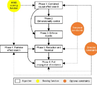
The Saiyan algorithm is based on a novel associational score that measures the level of difference between prior and posterior distributions. The algorithm follows a six-phase process to construct a DAG, with optional temporal and directed constraints, as illustrated in Fig 1. The high-level reasoning for each of the phases is as follows:
i. Phase 1 generates a graph based on the combined causal effect each pair of variables has on each remaining third variable. While the above process leads to multiple arcs between
nodes, only the arc that maximises a score function (refer to Section 2.1) is preserved for phase 2.
ii. Phase 2 ensures that model dimensionality is reasonably low relative to the input data. If a CPT has an expected parameter size greater than the sample size of the data, the weakest parent of that CPT is pruned until the dimensionality space is deemed acceptable.
iii. Phase 3 prunes the weakest arc in a cycle until the graph becomes acyclic.
iv. Phase 4 generates a new set of scores that are based on pairwise effect, rather than on the combined causal effect, and which are considered for further graphical modifications in subsequent phases.
v. Phase 5 uses the scores from phase 4 to simplify the graph via arc removals and arc reversals.
vi. Phase 6 connects any independent nodes, or graphical fragments, to enable full propagation of evidence.
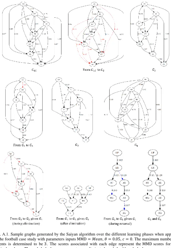
Fig A1 illustrates some of the graphical structures generated at different learning phases of the Saiyan algorithm. The outputs are based on the results of the Football case study (refer to Section 3.1). The subsections that follow describe the scoring function as well as each of the six phases in turn.
Fig. 1. The overall process of the Saiyan algorithm. 2.1 The MMD scoring function
The scoring function investigated in this paper is called the Mean/Max/MeanMax Marginal Discrepancy (MMD). This score can be used to return either the average Mean (MN), average Max (MX), or average MeanMax (MM) discrepancies between marginal probabilities in prior and posterior distributions. The preferred type of discrepancy is specified as a parameter input. A higher discrepancy score between prior and posterior distributions indicates a stronger dependency.
If we assume discrepancy type MN to compute the score of B being a parent of A, the output will be the average over i distributional differences of mean marginal discrepancies between 𝑃(𝐴) and 𝑃(𝐴|𝑏𝑖); i.e., MMD𝑀𝑁(𝐴 ← 𝐵) is
(∑ [(∑|𝑃(𝑎𝑗) − 𝑃(𝑎𝑗|𝑏𝑖)| 𝑠𝐴 𝑗 ) 𝑠⁄ ]𝐴 𝑠𝐵 𝑖 ) 𝑠⁄ 𝐵 (1)
for each state 𝑎𝑗 in 𝐴 and 𝑏𝑖 in 𝐵, and over 𝑠𝐴 states in 𝐴 and 𝑠𝐵 states in 𝐵. In the case of MX, the
score is simply the average maximum, rather than the average mean, discrepancy between marginal probabilities. In the case of MM, the score is the average of MN and MX scores.
Consider the hypothetical prior and posterior distributions shown in Table 1. The mean marginal discrepancy, for example, between 𝑃(𝐴) and 𝑃(𝐴|𝑏1) is 0.025, whereas the maximum
marginal discrepancy is 0.05. Based on these discrepancies, and over all three discrepancy assessments between 𝑃(𝐴) and 𝑃(𝐴|𝑏𝑖), the three MMD scores are:
MMD𝑀𝑁(𝐴 ← 𝐵) =(0.025 + 0.05 + 0.15)⁄ = 0.0753 MMD𝑀𝑋(𝐴 ← 𝐵) =(0.05 + 0.1 + 0.25)⁄ = 0.13333
MMD𝑀𝑀(𝐴 ← 𝐵) =(0.075 + 0.1333)⁄ = 0.10422
Table 1. Hypothetical Prior and Posterior distributions used to illustrate the computation of the three different types of the MMD score.
𝑃(𝐴) 𝑃(𝐴|𝑏1) 𝑃(𝐴|𝑏2) 𝑃(𝐴|𝑏3)
𝑎1 0.10 0.05 0.1 0.05
𝑎2 0.25 0.30 0.2 0.40
𝑎3 0.35 0.35 0.3 0.10
𝑎4 0.30 0.30 0.4 0.45
2.2 Phase 1: Combined causal effect search
At phase 1, the algorithm searches over all possible 𝐶 → 𝐴 ← 𝐵 structures to measure the MMD
score each pair of parents {𝐵, 𝐶} has on each residual data variable 𝐴. For example, the score
MMD𝑀𝑁(𝐶 → 𝐴 ← 𝐵 ) is (∑ ∑ [(∑|𝑃(𝐴𝑗) − 𝑃(𝐴𝑗|𝐵𝑖, 𝐶𝑘)| 𝑠𝐴 𝑗 ) 𝑠⁄ ]𝐴 𝑠𝐵 𝑖 𝑠𝐶 𝑘 ) (𝑠⁄ 𝐵+ 𝑠𝐶) (2)
The resulting score is assigned to both arcs entering 𝐴, from 𝐵 and 𝐶, as long as the discrepancy score is greater than the threshold 𝜃 specified by the user; otherwise, the arcs are not drawn.
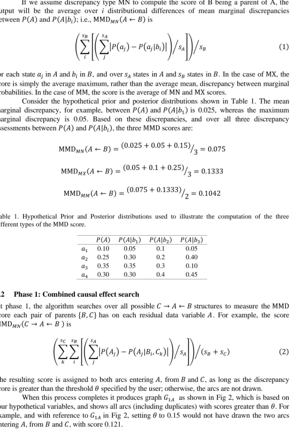
When this process completes it produces graph 𝐺1𝐴 as shown in Fig 2, which is based on
four hypothetical variables, and shows all arcs (including duplicates) with scores greater than 𝜃. For example, and with reference to 𝐺1𝐴 in Fig 2, setting 𝜃 to 0.15 would not have drawn the two arcs
Graph 𝐺1𝐴 is then revised into 𝐺1𝐵 by eliminating duplicate arcs and preserving the
maximum score over all duplicates. A third revision follows, that produces graph 𝐺1𝐶 from 𝐺1𝐵,
in which bi-directions are eliminated by preserving the direction that maximises MMD, as illustrated in Fig 2. Algorithm 1 describes this process, with optional code to account for temporal and directed knowledge-based constraints highlighted in grey.
Fig. 2. The three subphases of phase 1, based on hypothetical data. Red dashed arcs represent arcs eliminated.
ALGORITHM 1: Phase 1, with optional code for knowledge-based constraints in grey shading. Input: variables 𝑥, discrepancy threshold 𝜃
Output: graph 𝐺1𝐶
// Produce graph 𝐺1𝐴 in phase 1.
List 𝐿
for each variable 𝑥𝑖∈𝑥do
for each remaining variable 𝑥𝑗∈𝑥do
for each remaining variable 𝑥𝑘∈𝑥do
if 𝑥𝑖 ← 𝑥𝑗 and 𝑥𝑖← 𝑥𝑘 satisfy constraints then
add MMD ቀ𝑃(𝑥𝑖), 𝑃(𝑥𝑖|𝑥𝑗, 𝑥𝑘)ቁ score 𝑠 in 𝐿 if 𝑠 > 𝜃
end if end for end for end for
// Produce graph 𝐺1𝐵 in phase 1, revised from 𝐺1𝐴.
for each 𝑠∈𝐿do
𝑠 = 1 end if
Eliminate duplicate arcs and preserve max(𝑠) end for
// Produce graph 𝐺1𝐶 in phase 1, revised from 𝐺1𝐵.
for each 𝑠∈𝐿do
Eliminate the bi-directed arc with the lowest 𝑠2
end for
2.3 Phases 2 and 3: Dimensionality and Acyclic
At phase 2, the algorithm determines the maximum number of parents a node can have, as described in Algorithm 2. The maximum number of parents is determined by CPT size relative to the sample size of the input data. This process ensures that the expected number of parameters of the average CPT with 𝑎 parents will not be greater than the sample size of the data. Setting parameter input 𝑐 = 1 represents a more conservative choice where the maximum number of parents further decreases by
1.
Once the maximum number of parents is determined, the algorithm revises 𝐺1𝐶 into 𝐺2 by
pruning the excess parents that violate this restriction, starting from the weakest parent in terms of
MMD score. For a visual example, refer to the first three graphs in Fig A1 where the maximum number of parents is determined to be 3.
At phase 3, the algorithm searches for cycles in 𝐺2 and breaks them until the graph
becomes acyclic. This is achieved by removing the weakest arc in a cycle, one at a time, as determined by MMD score. This process is repeated until no cycles exist. The result is graph 𝐺3
(also as shown in Fig A1).
ALGORITHM 2: Determining max parents during phase 2. Input: user input 𝑐, sample size 𝑛, average states 𝑦̅
Output: 𝑎 𝑎 = 1
threshold = 1 c𝑜𝑛𝑣𝑒𝑟𝑔𝑒𝑛𝑐𝑒 = 2
whileconvergence > thresholddo convergence = 𝑛 𝑦̅(𝑎+2) ⁄ ifconvergence > thresholddo 𝑎 + + end if end while 𝑎 = 𝑎 − 𝑐
2.4 Phases 4 and 5: Pairwise effect search, Reduction and Reversal
As initially shown in Fig 1, phase 4 generates a new set of scores that are based on pairwise rather than combined causal effect, and these scores are used in subsequent phases to perform further graphical modifications. In computing the pairwise scores, phase 4 also produces the supplementary fully connected undirected graph 𝐺4, as shown in the example of Fig A1. If the MMD score is set to
type MN, then each undirected edge 𝐴 − 𝐵 in 𝐺4 is assigned the average MMD score of 𝐴 → 𝐵 and 𝐴 ← 𝐵; i.e., MMD𝑀𝑁(𝐴 − 𝐵) is
[MMD𝑀𝑁(𝐴 ← 𝐵) + MMD𝑀𝑁(𝐴 → 𝐵)] 2
⁄ (3)
Phase 5 begins by eliminating edges in the supplementary graph 𝐺4, one by one, starting
from the edge with the lowest score. As described in Algorithm 3, for each edge 𝐴 − 𝐵 eliminated, if 𝐴 and 𝐵 share neighbour 𝐶 (implying that edges 𝐴 − 𝐶 and 𝐵 − 𝐶 have MMD scores greater than that of 𝐴 − 𝐵), the ‘reduction’ step is activated. This step checks if the edge eliminated in 𝐺4 exists
in 𝐺3 as an arc and if yes, and assuming the edge eliminated in 𝐺4 is 𝐴 − 𝐵 and the respective arc in 𝐺3 is 𝐴 → 𝐵, then 𝐴 → 𝐵 is not preserved in 𝐺5 as long as:
i. 𝐴 − 𝐵 has MMD < 𝜃. In this case, the arc is eliminated since the pairwise score between
𝐴 and 𝐵 is lower than threshold 𝜃.
ii. 𝐴 and 𝐵 in 𝐺3 share a neighbour 𝐶 that is not a child of 𝐴 and 𝐵. In this case, the arc is
eliminated since the dependency is preserved through 𝐶.
iii. 𝐴 and 𝐵 in 𝐺3 share child 𝐶. In this case, 𝐴 → 𝐵 is not preserved from 𝐺3 to 𝐺5, and
further activates the ‘reversal’ step. Specifically, for each 𝐴 → 𝐵 not preserved in 𝐺5, if 𝐴
and 𝐵 share child 𝐶, then 𝐴 → 𝐶 ← 𝐵 is reoriented into 𝐴 → 𝐶 → 𝐵 (or 𝐴 ← 𝐶 ← 𝐵 in the case of 𝐴 ← 𝐵) as long as the graph remains acyclic and optional knowledge-based constraints are not violated.
ALGORITHM 3: Phases 4 and 5, with optional knowledge-based constraints in grey shading. Input: variables 𝑋, discrepancy threshold 𝜃, graph 𝐺3
Output: graphs 𝐺4 and 𝐺5
// Produce graph 𝐺4 in phase 4, independent of 𝐺3.
for each variable 𝑥𝑖∈𝑋do
for each remaining variable 𝑥𝑗∈𝑋do
if 𝑥𝑖 and 𝑥𝑗 are part of a directed constraint then
add them in 𝐺4 with MMD score 1
else add them in 𝐺4 with MMD score [MMD ቀ𝑃(𝑥𝑖), 𝑃(𝑥𝑖|𝑥𝑗)ቁ + MMD ቀ𝑃(𝑥𝑗), 𝑃(𝑥𝑗|𝑥𝑖)ቁ] 2⁄
end if end for end for
// Produce graph 𝐺5 in phase 5, dependent on 𝐺3 and 𝐺4.
while edge 𝑒∈ 𝐺4 do
delete 𝑒𝑖 in 𝐺4with min(MMD) and get nodes 𝐴 and 𝐵
if 𝐴 and 𝐵 share a neighbour 𝐶 in 𝐺4then
if there is an arc between 𝐴 and 𝐵 in 𝐺3then
if 𝑒𝑖 had MMD < 𝜃
delete arc between 𝐴 and 𝐵 in in 𝐺5
else if𝐴 and 𝐵 share a non-child 𝐶 in 𝐺3then
delete arc between 𝐴 and 𝐵 in in 𝐺5
else if𝐴 and 𝐵 share a child 𝐶 in 𝐺3then
for each 𝐶do
if the arc eliminated in 𝐺5 was 𝐴 → 𝐵then
if 𝐴 → 𝐶 → 𝐵 do not violate constraints then
alter 𝐴 → 𝐶 ← 𝐵 to 𝐴 → 𝐶 → 𝐵 if 𝐺5 remains acyclic
end if else
if 𝐴 ← 𝐶 ← 𝐵 do not violate constraints then
alter 𝐴 → 𝐶 ← 𝐵 to 𝐴 ← 𝐶 ← 𝐵 if 𝐺5 remains acyclic
end if end if end for end if end if end if end while 2.5 Phase 6: DAG
The final phase ensures that the graph returned to the user is a DAG that enables full propagation of evidence. It starts by searching for the largest graphical fragment 𝑔5𝑖 in 𝐺5, and then for the
variable 𝑥𝑖 that is not part of 𝑔5𝑖 and which maximises MMD score on a variable 𝑧𝑖 in 𝑔5𝑖. It then
connects 𝑥𝑖 to 𝑧𝑖 with an arc. The direction of the arc is determined based on the number of
parents in 𝑥𝑖 with respect to 𝑧𝑖; i.e., the node with the lowest number of parents is selected as the
child (unless it violates any knowledge-based constraints). This process is repeated until all 𝑥𝑖
become part of 𝑔5𝑖. Algorithm 4 describes this phase.
ALGORITHM 4: Phase 6, with optional knowledge-based constraints in grey shading. Input: variables 𝑋, graph 𝐺4, graph 𝐺5
Output: graph 𝐺6
// Produce graph 𝐺6 in phase 6, dependent on 𝐺4 and 𝐺5.
Find the largest BN fragment 𝑔5𝑖∈ 𝐺5 and get variables 𝑍 of 𝑔5𝑖.
while size of set 𝑍 <size of set 𝑋do for each 𝑥𝑖∉ 𝑍do
Search for variable 𝑧𝑖 that maximises 𝑠 on a 𝑥𝑖
if𝑥𝑖 has parents ≥ to the number of parents of 𝑧𝑖then
if 𝑥𝑖→ 𝑧𝑖 does not violate constraints then
do 𝑥𝑖→ 𝑧𝑖
else do 𝑧𝑖→ 𝑥𝑖
end if else
if 𝑧𝑖→ 𝑥𝑖 does not violate constraints then
do 𝑧𝑖→ 𝑥𝑖 else do 𝑥𝑖→ 𝑧𝑖 end if end if end for end while
2.6 Computational and time complexity
Previous relevant studies have based computational complexity on the number of associational tests between variables, and the number of conditional independence tests [3], [14], [32]. As described in the previous subsections, the only phases that involve associational tests are phases 1 and 4 which compute the combined causal and pairwise MMD scores respectively. The remaining phases simply make use of those MMD scores to modify the graph.
More specifically, the number of associational tests in phase 1 is [𝑥(𝑥 − 1)(𝑥 − 2)] 2⁄ , where 𝑥 is the number of variables in the data. In phase 4, the number of associational tests is
𝑥(𝑥 − 1). Therefore, computational complexity is the sum of associational tests over these two phases; i.e.,
𝑂 (ቀ𝑥(𝑥 − 1)(𝑥 − 2)⁄ ቁ + 𝑥(𝑥 − 1))2
Due to the exhaustive search performed in phase 1, each increase in 𝑥 results in a non-linear cubic growth in the number of associational tests. This means that the Saiyan algorithm is not suitable for datasets that incorporate 1000s of variables, such as those in bioinformatics. Algorithms that scale linearly with the number of variables are typically more suitable for those problems.
3 EVALUATION AND RESULTS
The evaluation process is based on four case studies (10 datasets, including different sample sizes), four scoring metrics, and another ten state-of-the-art or well-established structure learning algorithms.
3.1 Data case studies
Two real-world and two synthetic case studies are considered. The real-world case studies represent a ‘simple’ and a ‘complex’ test, whereas the synthetic case studies represent a ‘rule-based’ and a ‘knowledge-based’ test. Specifically,
i. Football: A real-world dataset that consists of seven variables and has a sample size of 380. The data and knowledge-based BN graph are based on a simplified version of the model presented in [33]. This dataset represents the ‘simple’ real-world test.
ii. Forensic medicine: A real-world dataset that consists of 56 variables and has a sample size of 953. The data and knowledge-based graph are based on [34]. This dataset represents the ‘complex’ real-world test.
iii. Alarm network: The classic BN model that consists of 37 variables. Data are simulated based on the knowledge-based structure and parameters specified in the Bayesian Network Repository with reference to [35]. This dataset represents the ‘knowledge-based’ synthetic test.
iv. Property market: A rule-based BN model that consists of 27 variables and which had its structure and parameters determined by clearly defined rules and regulating protocols associated with the UK property market, as described in [36]. This dataset represents the ‘rule-based’ synthetic test.
It is important to note that for cases i and ii, the algorithms are judged in terms of how well they predict the knowledge-based graph, which is not necessarily the ground truth graph. For cases iii
and iv, the algorithms are judged in terms of how accurately they reconstruct the hypothetical ground truth graph.
3.2 Evaluation metrics
Four evaluation metrics are considered that are fully oriented towards graphical discovery. These are:
i. the classic F1 score which represents the harmonic mean of Precision and Recall; the most popular metrics used to evaluate BN structure learning algorithms in the literature [37], ii. the Structural Hamming Distance (SHD) metric that penalises each change required to
transform the discovered graph into the ground truth graph by 1 [14],
iii. the DAG Dissimilarity Metric (DDM) that penalises dissimilarities and rewards similarities between graphs, with a weighted reward for un/bi-directed edges [37],
iv. the Balanced Scoring Function (BSF) that balances the score proportional to the number of direct dependencies and independencies in the ground truth graph, by taking into consideration all of the confusion matrix parameters. A score of 0 represents performance equivalent to an empty or a fully connected graph, and scores of -1 and 1 represent the most inaccurate and accurate graphs respectively [37].
Note that, in thus study, all of the four metrics consider the discovery of a correct edge with an incorrect direction to be a partial match with a 50% reward. For example, if the true arc is 𝐴 → 𝐵
and an algorithm discovers 𝐴 → 𝐵, then the reward will be 1; but the reward will be 0.5 if the algorithm discovers 𝐴 ↔ 𝐵, 𝐴 − 𝐵, or 𝐴 ← 𝐵 instead (and 0 for no edge). Finally, the evaluation process assumes that the ground truth graph is a DAG, rather than a PDAG.
3.3 Structure learning algorithms considered
The TETRAD freeware and the bnlearn R Statistical package [38] were used to test the other algorithms. The graphs generated by the Saiyan algorithm are compared to the graphs generated by each of the other 10 algorithms when applied to the same data. The other 10 algorithms are:
i. The PC (Peter-Clark) algorithm, which uses conditional independence tests to construct the network and is perhaps the most well-known constraint-based algorithm [39].
ii. The FCI (Fast Causal Inference) algorithm, that is similar to PC but which accounts for the possibility of latent confounders [40].
iii. The FGES (Fast Greedy Equivalence Search) algorithm which is a parallelised and an optimised version of the score-based GES algorithm that was initially developed by Meek [41] and later further developed by Chickering [12].
iv. The GS (Grow-Shrink Markov Blanket) algorithm which recovers the Markov blanket based on pairwise independence test [38].
v. The MMPC (Max-Min Parents and Children) constraint-based algorithm that uses forward selection to discover neighbours based on the maximum and minimum associations observed in subset nodes during previous iteration [42].
vi. The HC (Hill-Climbing) score-based algorithm that searches the space of directed graphs using greedy search [43].
vii. The TABU (Tabu Search) scored-based algorithm that is a modified HC version designed to escape local optima [43].
viii. The MMHC (Max-Min Hill-Climbing) hybrid algorithm, which is based on MMPC and HC algorithms, and is said to outperform several prototypical and state-of-the-art algorithms [14].
ix. The IAMB (Incremental Association) constraint-based algorithm which is a Markov blanket detection algorithm using forward selection search [44].
x. The RSMAX2 (Restricted Maximization) hybrid algorithm which is a modified version of MMHC that uses different combinations of constraint-based and score-based searches [45, 46].
The TETRAD freeware version 6.5.3 was used to run the PC, FCI, and FGES algorithms with their default parameter inputs, and the bnlearn R Statistical package v4.4 was used to run the GS, MMPC, HC, TABU, MMHC, IAMB, and RSMAX2 algorithms with their default parameter inputs [46].
3.4 Results and discussion
The results are based on the four case studies discussed in Section 3.1, and on a total of 10 datasets. The 10 datasets are the result of dividing each of the two synthetic case studies into four datasets of different sample size; i.e., 0.1, 1, 10, and 100 thousand samples per dataset per synthetic case.
The Saiyan algorithm is tested over different combinations of parameter input. Specifically, 42 graphs are generated for each dataset, where each of those 42 graphs represents a unique combination of the following parameters:
i. Three types of MMD score to measure the discrepancy between prior and posterior distributions; i.e. MN, MX, and MM as defined in Section 2.1.
ii. Seven different discrepancy thresholds 𝜃, which represent the threshold above which a relationship is established between variables given the MMD score, as defined in Section 2.2. The seven thresholds tested are 0.05, 0.07, 0.1, 0.15, 0.2, 0.25, and 0.3.
iii. Two input values for constant 𝑐 (0 or 1), which modifies the maximum number of parents a node can have as defined in Section 2.3.
Since the evaluation is based on 10 datasets, a total of 100 graphs are generated by the other algorithms (one graph per dataset per algorithm), and 420 graphs are generated by the Saiyan algorithm (42 graphs per dataset). Therefore, the results from this evaluation illustrate how the Saiyan algorithm with unoptimised parameters (i.e., over 42 different parameter inputs) performs relative to the 10 algorithms with default parameters.
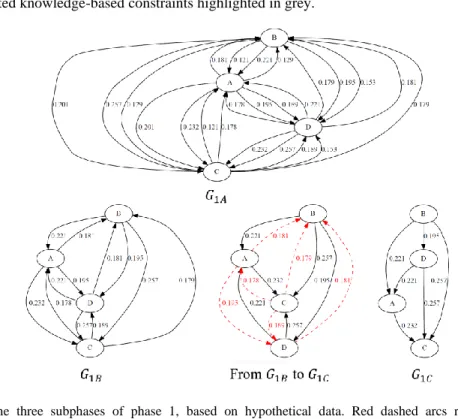
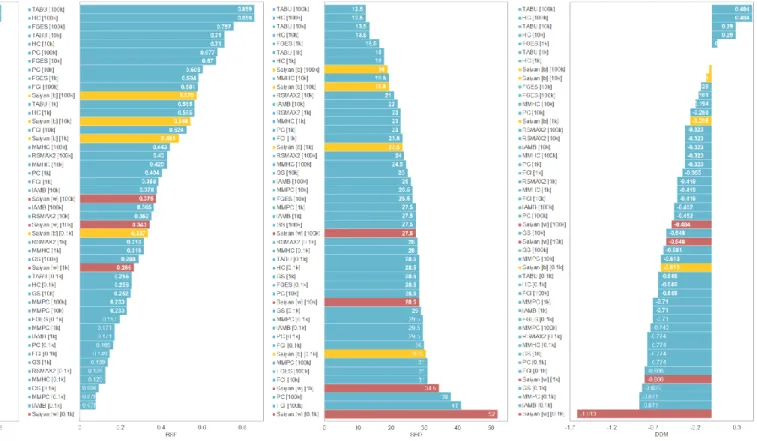
Figs 3 and 4 present the ranking of the algorithms, as determined by each of the four metrics, in terms of how well they predict the Football and Forensic medicine knowledge-based graphs. Two scores are reported for Saiyan; the best and worst scores over the 42 graphs generated per case study.
Fig. 3. Football case study: Performance of each algorithm as determined by each of the four metrics, in terms of how well they predict the knowledge-based graph. Algorithms Saiyan [b] and Saiyan [w] represent the best (highlighted in orange) and worst (highlighted in red) scores respectively, over the 42 parameter input combinations.
Fig. 4. Forensic medicine case study: Performance of each algorithm as determined by each of the four metrics, in terms of how well they predict the knowledge-based graph. Algorithms Saiyan [b] and Saiyan [w] represent the best (highlighted in orange) and worst (highlighted in red) scores respectively, over the 42 parameter input combinations.
Overall, the algorithms have done well in predicting the Football knowledge-based graph, but not well in predicting the more complex Forensic medicine graph. The same applies to the Saiyan algorithm. However, not being able to discover a graph that closely approximates the knowledge-based graph does not imply that the graph discovered is inaccurate. Still, these results suggest that the algorithms are rather consistent in the graphs they generate; at least in relation to the knowledge-based graphs.
Interestingly, while the four metrics are generally in agreement when it comes to ranking the algorithms in the Football case study, they generate conflicting rankings in the Forensic medicine
case study. The most staggering example involves the GS algorithm; F1 and BSF metrics place GS at the bottom of the rankings whereas SHD and DDM metrics place GS at the top of the rankings. This inconsistency occurs because the GS generates a limited number of edges relative to the other algorithms (refer to Table 2). The limited number of edges is viewed positively by the SHD and DDM metrics which approximate classification accuracy and hence, tend to be biased in favour of empty graphs [37].
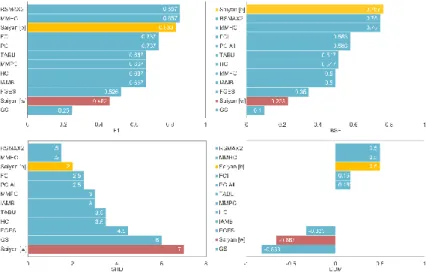
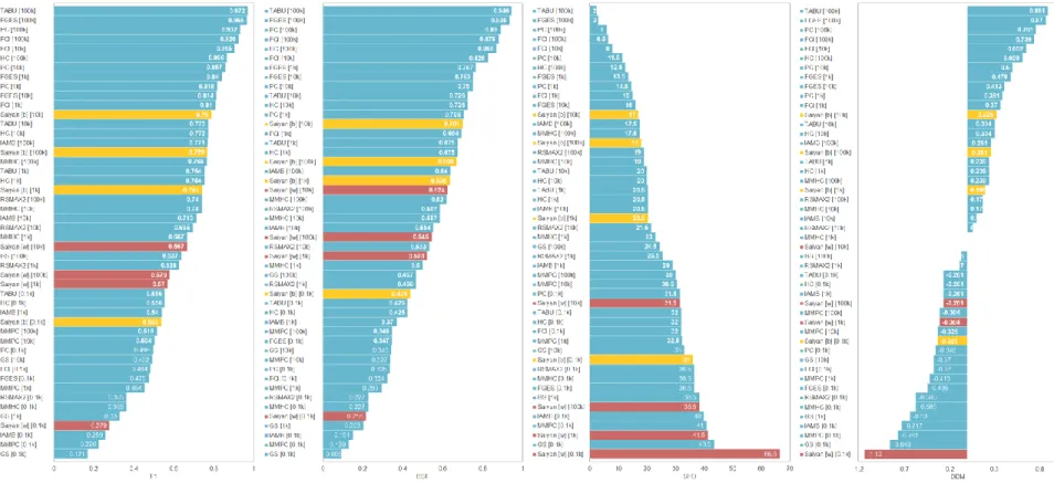
Similarly, Figs 5 and 6 rank the synthetic performance of the algorithms for the Property market and Alarm network case studies respectively. These graphs include the performance scores over all of the four different data sample sizes. Results of interest include:
i. The TABU algorithm has topped all of the rankings and is closely followed by the similar HC algorithm.
ii. While the Saiyan algorithm has not topped any of the rankings, its performance is competitive relative to most of the other algorithms.
iii. The F1 (Recall and Precision) and BSF metrics tend to rank the Saiyan algorithm higher than the SHD and DDM metrics.
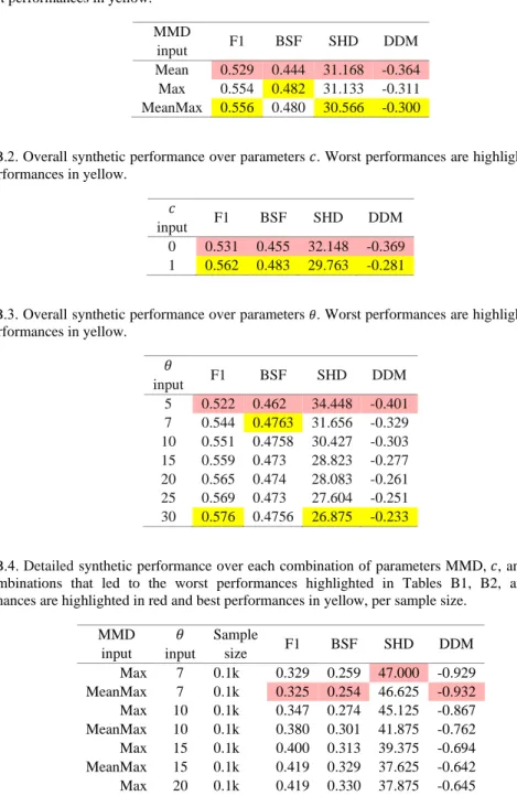
iv. The worst performances of the Saiyan algorithm (i.e., Saiyan [b]) are often at the bottom of the rankings. This suggests that some of the parameter inputs tested, which are detailed in Appendix B, are far from being optimal and should be avoided. Tables B1, B2, and B3 suggest that the inputs ‘Mean’, ‘5’, and ‘0’ for respective parameters MMD, 𝜃, and 𝑐, produce scores that are considerably inferior relative to the scores generated when based on the remaining parameter inputs tested. According to Table B4, however, even when we restrict the results to the better performing parameter inputs, it is still unclear which combination of inputs maximises performance over all cases. It is possible that the optimal parameters depend on the dimensionality of the data relative to the sample size of the input data.
v. Increasing the sample size of the input data does not always improve accuracy. This observation applies to multiple algorithms, and applies to both synthetic case studies. However, in most cases the difference in scoring performance is rather marginal and may be due to random variability that arises once an algorithm is provided with enough data samples.
vi. The results are not entirely consistent with those reported in [14], in which the MMHC outperforms several prototypical algorithms according to the SHD score, including the PC, GES, and GS algorithms tested in this paper. The RSMAX2 algorithm, which is a modified version of MMHC, appears to be on par with MMHC, as expected.
Table 2 presents the number of arcs or edges discovered by each of the algorithms, as well as the number of independent graphical fragments (i.e., disjoint subgraphs) or variables generated by each of the algorithms, for each case study. Observations of interest include:
i. The other algorithms will rarely return a graph that enables full propagation of evidence, despite all of the input variables being dependent.
ii. The number of edges generated by the Saiyan algorithm appear to better approximate the knowledge-based or true number of edges. For example, in the Forensic medicine case none of the other algorithms came close to generating 103 edges. Remarkably, the GS algorithm only discovered 9 edges and yet, the SHD and DDM metrics considered GS to be the best performing algorithm (refer to Fig 4). This observation serves as further evidence that simple classification accuracy, which these metrics approximate, can be
misleading. Moreover, five of the other algorithms (GS, MMHC, IAMB, MMPC, and RSMAX2) also generated a low number of edges relative to the true number of edges, for both synthetic experiments and irrespective of sample size.
iii. In the Property market case study, the variability in the number of edges discovered is minor for the Saiyan algorithm (over its 168 graphs), whereas it is much higher for the other algorithms (over just four graphs; one per sample size). This difference is relaxed in the Alarm network case. Overall, these results suggest that Saiyan is more consistent in the number of edges discovered, which is a consequence of the assumption that all of the input variables are dependent.
iv. While the restriction to enable full propagation of evidence is expected to lead to more complex graphs, Table 2 suggests that this is often, but not always, the case. For example, in the Property market case the PC, FCI and FGES algorithms generated a much higher number of edges across all four sample size cases, compared to the Saiyan’s maximum number of edges generated across all of the 168 different graphs. This observation, however, does not extend to the Alarm network case. Moreover, most of the other algorithms tend to generate simple models with limited edges when the sample size is low.
Fig. 5. Property market case study: Performance of each algorithm over different sample sizes, as determined by each of the four metrics, in terms of how well they predict the hypothetical ground truth rule-based graph. Algorithms Saiyan [b] and Saiyan [w] represent the best (highlighted in orange) and worst (highlighted in red) scores respectively, over the 42 parameter input combinations, per sample size.
Fig. 6. ALARM network case study: Performance of each algorithm over different sample sizes, as determined by each of the four metrics, in terms of how well they predict the hypothetical ground truth graph. Algorithms Saiyan [b] and Saiyan [w] represent the best (highlighted in orange) and worst (highlighted in red) scores respectively, over the 42 parameter input combinations, per sample size.
Table 2. The number of edges and independent graphical fragments (or disjoint subgraphs) discovered per algorithm per case study.
Case Variables True
arcs Algorithms Graphs generated Edges discovered
Independent graphical fragments Football 7 6 Saiyan 42 6 to 9 1 PC 1 6 1 FCI 1 6 1 FGES 1 6 1 GS 1 3 4 MMHC 1 6 1 IAMB 1 6 1 HC 1 6 1 MMPC 1 6 1 TABU 1 6 1 RSMAX2 1 6 1 Forensic medicine 56 103 Saiyan 42 55 to 111 1 PC 1 69 7 FCI 1 69 7 FGES 1 76 5 GS 1 9 47 MMHC 1 39 19 IAMB 1 44 17 HC 1 72 4 MMPC 1 43 18 TABU 1 72 4 RSMAX2 1 39 20 Property market 27 31 Saiyan 168 26 to 29 1 PC 4 13 to 57 3 to 15 FCI 4 13 to 57 3 to 15 FGES 4 16 to 56 1 to 11 GS 4 7 to 20 9 to 20 MMHC 4 5 to 24 8 to 22 IAMB 4 6 to 23 9 to 21 HC 4 15 to 37 1 to 12 MMPC 4 6 to 24 9 to 21 TABU 4 15 to 37 1 to 12 RSMAX2 4 5 to 22 9 to 22 Alarm network 37 46 Saiyan 168 36 to 57 1 PC 4 21 to 45 2 to 16 FCI 4 21 to 45 2 to 16 FGES 4 30 to 45 2 to 10 GS 4 11 to 26 12 to 26 MMHC 4 13 to 32 7 to 24 IAMB 4 13 to 33 6 to 24 HC 4 31 to 51 2 to 7 MMPC 4 13 to 32 7 to 24 TABU 4 31 to 45 2 to 7 RSMAX2 4 13 to 30 9 to 24
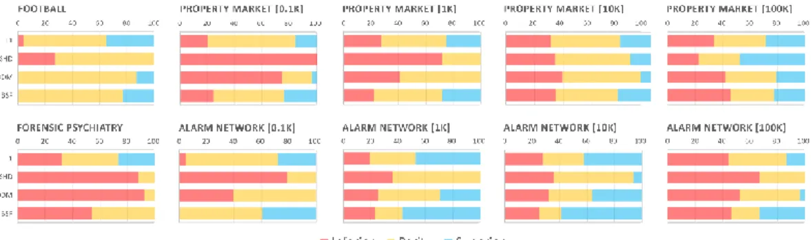
Fig. 7. Overall performance of the Saiyan algorithm (over all 42 input unoptimised combinations) relative to the overall performance of the other 10 algorithms. The bars illustrate the percentage of the Saiyan’s scores being inferior, on par, and superior, relative to the respective scores generated by the other 10 algorithms. 4 CONCLUDING REMARKS AND FUTURE WORK
This paper presented a BN structure learning algorithm, called Saiyan, which is based on a novel scoring function to determine relationships between variables, and follows an unconventional six-phase associational heuristic approach to generate a DAG that enables full propagation of evidence.
In guaranteeing full propagation of evidence, Saiyan ‘forces’ the discovery of edges that would otherwise remain undiscovered, and these additional edges are not expected to be correct at the rate of those identified unrestrictedly. The assumption that the input variables are dependent is a practical solution and not a theoretical advancement, which means that the restriction may negatively impact the evaluation scores. Moreover, Saiyan represents an associational heuristic that, in theory, is not expected to perform well relative to more sophisticated approaches, such as those based on constraint-based and score-based learning. Still, the empirical results suggest that this heuristic is as competitive as the average algorithm evaluated in this study.
The Saiyan algorithm represents an experimental implementation. Planned extensions of this research will investigate the impact of the assumption to enable full propagation of evidence on constraint-based and score-based learning. The latest version of the Saiyan algorithm, along with relevant datasets and Bayesian Network case studies, is available online [47] .
ACKNOWLEDGMENTS
This research was supported by the ERSRC Fellowship project EP/S001646/1 on Bayesian Artificial Intelligence for Decision Making under Uncertainty, and by The Alan Turing Institute in the UK.
APPENDIX A: SAMPLE GRAPHS GENERATED BY SAIYAN
Fig. A.1. Sample graphs generated by the Saiyan algorithm over the different learning phases when applied to the football case study with parameters inputs MMD = 𝑀𝑒𝑎𝑛, 𝜃 = 0.05, 𝑐 = 0. The maximum number of parents is determined to be 3. The scores associated with each edge represent the MMD scores for the particular phase. The red dashed arcs represent arcs eliminated, and the blue dashed arcs represent arcs reversed.
APPENDIX B: SYNTHETIC PERFORMANCE SAIYAN BASED ON DIFFERENT PARAMETER INPUTS
Table B.1. Overall synthetic performance over parameters MMD. Worst performances are highlighted in red and best performances in yellow.
MMD
input F1 BSF SHD DDM
Mean 0.529 0.444 31.168 -0.364 Max 0.554 0.482 31.133 -0.311 MeanMax 0.556 0.480 30.566 -0.300
Table B.2. Overall synthetic performance over parameters 𝑐. Worst performances are highlighted in red and best performances in yellow.
𝑐
input F1 BSF SHD DDM
0 0.531 0.455 32.148 -0.369 1 0.562 0.483 29.763 -0.281
Table B.3. Overall synthetic performance over parameters 𝜃. Worst performances are highlighted in red and best performances in yellow.
𝜃 input F1 BSF SHD DDM 5 0.522 0.462 34.448 -0.401 7 0.544 0.4763 31.656 -0.329 10 0.551 0.4758 30.427 -0.303 15 0.559 0.473 28.823 -0.277 20 0.565 0.474 28.083 -0.261 25 0.569 0.473 27.604 -0.251 30 0.576 0.4756 26.875 -0.233
Table B.4. Detailed synthetic performance over each combination of parameters MMD, 𝑐, and 𝜃, excluding the combinations that led to the worst performances highlighted in Tables B1, B2, and B3. Worst performances are highlighted in red and best performances in yellow, per sample size.
MMD input 𝜃 input Sample size F1 BSF SHD DDM Max 7 0.1k 0.329 0.259 47.000 -0.929 MeanMax 7 0.1k 0.325 0.254 46.625 -0.932 Max 10 0.1k 0.347 0.274 45.125 -0.867 MeanMax 10 0.1k 0.380 0.301 41.875 -0.762 Max 15 0.1k 0.400 0.313 39.375 -0.694 MeanMax 15 0.1k 0.419 0.329 37.625 -0.642 Max 20 0.1k 0.419 0.330 37.875 -0.645 MeanMax 20 0.1k 0.427 0.337 37.125 -0.623 Max 25 0.1k 0.433 0.345 37.125 -0.610 MeanMax 25 0.1k 0.430 0.337 36.625 -0.612 Max 30 0.1k 0.436 0.345 36.625 -0.599
MeanMax 30 0.1k 0.435 0.343 36.500 -0.599 Max 7 1k 0.582 0.514 29.500 -0.232 MeanMax 7 1k 0.575 0.510 30.500 -0.257 Max 10 1k 0.587 0.515 28.750 -0.218 MeanMax 10 1k 0.561 0.489 30.750 -0.289 Max 15 1k 0.572 0.494 29.000 -0.253 MeanMax 15 1k 0.537 0.462 31.625 -0.348 Max 20 1k 0.576 0.493 28.750 -0.243 MeanMax 20 1k 0.548 0.464 30.125 -0.315 Max 25 1k 0.574 0.490 28.500 -0.245 MeanMax 25 1k 0.545 0.459 30.000 -0.323 Max 30 1k 0.577 0.491 27.875 -0.237 MeanMax 30 1k 0.569 0.478 27.750 -0.258 Max 7 10k 0.645 0.589 25.000 -0.053 MeanMax 7 10k 0.676 0.607 22.375 0.033 Max 10 10k 0.647 0.592 24.875 -0.048 MeanMax 10 10k 0.666 0.596 23.000 0.006 Max 15 10k 0.668 0.592 22.375 0.009 MeanMax 15 10k 0.660 0.584 22.875 -0.007 Max 20 10k 0.661 0.584 22.625 -0.007 MeanMax 20 10k 0.661 0.561 21.750 -0.012 Max 25 10k 0.666 0.580 21.875 0.004 MeanMax 25 10k 0.642 0.539 22.500 -0.061 Max 30 10k 0.653 0.554 21.875 -0.034 MeanMax 30 10k 0.651 0.546 21.750 -0.039 Max 7 100k 0.657 0.593 24.250 -0.024 MeanMax 7 100k 0.650 0.589 25.125 -0.046 Max 10 100k 0.660 0.597 24.125 -0.016 MeanMax 10 100k 0.656 0.577 23.625 -0.024 Max 15 100k 0.633 0.540 24.000 -0.086 MeanMax 15 100k 0.650 0.557 22.875 -0.040 Max 20 100k 0.645 0.552 23.000 -0.053 MeanMax 20 100k 0.663 0.569 22.000 -0.007 Max 25 100k 0.650 0.548 22.250 -0.042 MeanMax 25 100k 0.656 0.560 22.250 -0.026 Max 30 100k 0.659 0.549 21.250 -0.021 MeanMax 30 100k 0.674 0.564 20.250 0.018
REFERENCES
[1] Judea Pearl, “Reverend Bayes on Inference Engines: A Distributed Hierarchical Approach”, In Proceedings of the 2nd
AAAI Conference on Artificial Intelligence, pp. 133–136, Pittsburgh, Pennsylvania, August 1982. AAAI Press, 1982. [2] Judea Pearl, “Bayesian Networks: A model of self-activated memory for evidential reasoning”, In Proceedings of the
7th Conference of the Cognitive Science Society, pp. 329–334, 1985.
[3] Peter Spirtes, Clark Glymour and Richard Scheines, Causation, Prediction, and Search: 2nd Edition, The MIT Press,
Cambridge Massachusetts, and London, England, 2000.
[4] Steen A. Andersson, David Madigan and Michael D, “A characterization of Markov equivalence classes for acyclic digraphs”, Annals of Statistics, vol. 25, pp. 505–541, 1997.
[5] Christopher Meek, “Causal inference and causal explanation with background knowledge”, In Proceedings of the 11th
UAI Conference on Uncertainty in Artificial Intelligence, pp. 403–410, 1995.
[6] Peter Spirtes and Christopher Meek, “Learning Bayesian Networks with discrete variables from data”, In Proceedings of the 1st Annual Conference on Knowledge Discovery and Data Mining, pp. 294–299, 1995.
[7] David M. Chickering, David Heckerman and Christopher Meek, „Large-sample learning of Bayesian networks is NP-hard”, Journal of Machine Learning Research, vol. 5, pp. 1287–1330, 2004.
[8] Daphne Koller and Nir Friedman, “Probabilistic Graphical Models”, Cambridge, Massachusetts and London, England, The MIT Press, 2009.
[9] Gregory F. Cooper and Edward Herskovits, “A Bayesian method for the induction of probabilistic networks from data”, Machine Learning, vol. 9, pp. 309–347, 1992.
[10] Nir Friedman, Iftach Nachman and Dana Peer, “Learning Bayesian network structure from massive datasets: the “Sparse Candidate” algorithm”, In Proceedings of the 16th UAI Conference on Uncertainty in Artificial Intelligence,
pp. 206–215, 1999.
[11] Andrew Moore and Weng-Keen Wong, “Optimal Reinsertion: A new search operator for accelerated and more accurate Bayesian network structure learning”, In Proceedings of the 20th International Conference on Machine
Learning (ICML), pp. 552–559, Washington DC, 2003.
[12] David M. Chickering, “Optimal structure identification with greedy search”, Journal of Machine Learning Research, vol. 3, pp. 507–554, 2002.
[13] Thomas Verma and Judea Pearl, “Equivalence and synthesis of causal models”, In Proceedings of the 6th UAI
Conference on Uncertainty in Artificial Intelligence, pp. 255–270, 1990.
[14] Ioannis Tsamardinos, Laura E. Brown and Constantin F. Aliferis, “The Max-Min Hill-Climbing Bayesian Network Structure Learning Algorithm”, Machine Learning, vol.65, pp. 31–78, 2006.
[15] Mark Schmidt, Alexandru Niculescu-Mizil and Kevin Murphy, “Learning graphical model structure using L1-regularization paths”, In Proceedings of the National Conference on Artificial Intelligence, pp. 1278–1283, 2007. [16] James Cussens, “Bayesian network learning with cutting planes”, In Fabio G. Cozman and Avi Pfeffer, editors,
Proceedings of the 27th Conference on Uncertainty in Artificial Intelligence (UAI 2011), pp. 153–160. AUAI Press, 2011.
[17] James Cussens, Matti Jarvisalo, Janne H. Korhonen, and Mark Bartlett, “Bayesian Network Structure Learning with Integer Programming: Polytopes, Facets and Complexity”, In Proceedings of the 26th International Joint Conference
on Artificial Intelligence (IJCAI-17), pp. 4990–4994, 2017.
[18] Mark Bartlett and James Cussens, “Integer linear programming for the Bayesian network structure learning problem”, Artificial Intelligence, vol. 244, pp. 258–271, 2017.
[19] Pekka Parviainen, Hossein Shahrabi Farahani, and Jens Lagergren, “Learning Bounded Tree-width Bayesian Networks using Integer Linear Programming”, In Proceedings of the 17th International Conderence on AI and
Statistics (AISTATS 2014), pp. 751–759.
[20] Tommi Jaakkola, David Sontag, Amir Globerson, and Marina Meila, “Learning Bayesian Network structure using LP relaxations”, In Proceedings of the 13th International Conference on Artificial Intelligence and Statistics (AISTATS
2010), pp. 358–365, 2010.
[21] Raymond Hemmecke, Silvia Lindner, and Milan Studeny, “Characteristic imsets for learning Bayesian network structure”, International Journal of Approcimate Reasoning, vol. 53, iss. 9, pp. 1336–1349.
[22] Robert Peharz and Franz Pernkopf, “Exact maximum margin structure learning of Bayesian networks”, In Proceedings of the 29th International Conference on Machine Learning (ICML 2012), Edinburgh, Scotland, UK,
2012.
[23] Tomi Silander and Petri Myllymaki, “A simple approach for finding the globally optimal Bayesian Network structure”, In Proceedings of the 22nd Conference on Uncertainty in Artificial Intelligence (UAI 2006), AUAI Press,
2006.
[24] Mikko Koivisto and Kismat Sood, “Exact Bayesian Structure Discovery in Bayesian Networks”, Journal of Machine Learning Research, vol. 5, pp. 549–573, 2004.
[25] Sascha Ott, Seiya Imoto, and Satoru Miyano, “Finding Optimal Models for Small Gene Networks”, In Pacific Symposium in Biocomputing, pp. 557–567, 2004.
[26] Ajit P. Singh and Andrew W. Moore, “Finding Optimal Bayesian Networks by Dynamic Programming”, Technical Report, CMU-CALD-05-106, Carnegie Mellon University, 2005.
[27] Changhe Yuan and Brandon Malone, “Learning optimal Bayesian Networks: A shortest path perspective”, Journal of Artificial Intelligence Research, vol. 48, pp23–65, 2013.
[28] Brandon Malone, Changhe Yuan, Eric A. Hansen, and Susan Bridges, “Improving the Scalability of Optimal Bayesian Network Learning with External-Memory Frontier Breadth-First Branch and Bound Search”, In Proceedings of the 27th Conference on Uncertainty in Artificial Intelligence (UAI 2011), pp. 479–488, 2011.
[29] Cassio de Campos and Qiang Ji, “Efficient Structure Learning of Bayesian Networks using Constraints”, Journal of Machine Learning Research, vol. 12, pp. 663–689, 2011.
[30] Seiya Imoto, Takao Goto, and Satoru Miyano, “Estimation of genetic networks and dunctional structures between genes by using Bayesian Networks and nonparametric regression”, In Pacific Symposium on Biocomputing, pp. 175-186, 2001.
[31] Peter van Beek and Hella-Franziska Hoffmann, “Machine learning of Bayesian networks using constraint programming”, In Gilles Pesant, editor, Proceedings of the 21st International Conference on Principles and Practice of Constraint Programming (CP 2015), vol. 9255 of Lecture Notes in Computer Science, pp. 429–445, 2015. [32] Dimitris Margaritis and Sebastian Thrun, “Bayesian network induction vial local neighborhoods”, In Advances in
Neural Information Processing Systems 12 (NIPS), pp. 505–512, 1999.
[33] Anthony C. Constantinou. “Asian handicap football betting with rating-based hybrid Bayesian networks”. arXiv:2003.09384 [stat.AP], 2019.
[34] Anthony C. Constantinou, Mark Freestone, William Marsh, Norman Fenton, and Jeremy Coid, “Risk assessment and risk management of violent reoffending among prisoners”, Expert Systems with Applications, vol. 42, no. 21, pp. 7511–7529, 2015.
[35] Ingo A. Beinlich, Jaap Suermondt, Martin Chavez, and Gregory F. Cooper, „The ALARM monitoring system: A case study with two probabilistic inference techniques for belief networks“, In Proceedings of the 2nd European Conference on Artificial Intelligence and Medicine, Berlin, Germany, 1989.
[36] Anthony C. Constantinou and Norman Fenton, “The future of the London Buy-To-Let property market: Simulation with Temporal Bayesian Networks”, PlOS ONE, vol. 12, no. 6, e0179297, 2017.
[37] Anthony C. Constantinou, “Evaluating structure learning algorithms with a balanced scoring function”, arXiv: 1905.12666, 2019.
[38] Marco Scutari, “Learning Bayesian Networks with the bnlearn R Package”, Journal of Statistical Software, vol. 35, no. 3, pp. 1–22.
[39] Peter Spirtes and Clark Glymour, “An algorithm for fast recovery of sparse causal graphs”, Social Science Computer Review, vol. 9, no. 1, 1991.
[40] Peter Spirtes, Christopher Meek, and Thomas Richardson, “An algorithm for causal inference in the presence of latent variables and selection bias”, In Clark Glymour and Gregory Cooper (Eds.), Computation, Causation, and Discovery. The MIT Press, Cambridge, MA, pp. 211–252, 1999.
[41] Christopher Meek, “Graphical Models: Selecting causal and statistical models”, PhD dissertation, Carnegie Mellon University, 1997.
[42] Ioannis Tsamardinos, Constantin F. Aliferis, and Alexander Statnikov, “Time and Sample Efficient Discovery of Markov Blankets and Direct Causal Relations”, In Proceedings of the Ninth ACM SIGKDD International Conference on Knowledge Discovery and Data Mining, pp. 673–678, 2003.
[43] Stuart Russell and Peter Norvig, “Artificial Intelligence: A Modern Approach”, Prentice Hall, 3rd Edition, 2009. [44] Ioannis Tsamardinos, Constantin F. Aliferis, and Alexander Statnikov, “Algorithms for Large Scale Markov Blanket
Discovery”, In Proceedings of the Sixteenth International Florida Artificial Intelligence Research Society Conference, pp. 376–381, 2003.
[45] Maxime Gasse, Alex Aussem, and Haytham Elghazel, “A hybrid algorithm for Bayesian network structure learning with application to multi-label learning”, Expert Systems with Applications, vol. 41, no. 15, pp. 6755–6772, 2014. [46] Marco Scutari and Jean-Baptiste Denis, Bayesian Networks: With examples in R, CRC Press, 2014.
[47] Anthony C. Constantinou. “The Bayesys user manual”. Queen Mary University of London, London, UK. [Online] Available at http://bayesian-ai.eecs.qmul.ac.uk/bayesys/ or http://www.bayesys.com