Department of Economics
University of Copenhagen
00-20
Explaining Cointegration Analysis: Part II
David F. Hendry
Katarina Juselius
Studiestræde 6, DK-1455 Copenhagen K., Denmark
Tel. +45 35 32 30 82 - Fax +45 35 32 30 00
David F. Hendry
Department of Economics, Oxford University, UK and
Katarina Juselius
Department of Economics, University of Copenhagen, Denmark November 12, 2000
Abstract We describe the concept of cointegration, its implications in modelling and forecasting, and discuss inference procedures appropriate in integrated-cointegrated vector autoregressive processes (VARs). Particular attention is paid to the properties of VARs, to the modelling of deterministic terms, and to the determination of the number of cointegration vectors. The analysis is illustrated by empirical examples.
1 Introduction
Hendry and Juselius (2000) investigated the properties of economic time series that were integrated processes, such as random walks, which contained a unit root in their dynamics. Here we extend the analysis to the multivariate context, and focus on cointegration in systems of equations.
We showed in Hendry and Juselius (2000) that when data were non-stationary purely due to unit roots (integrated once, denotedI(1)), they could be brought back to stationarity by the linear transform-ation of differencing, as inxt−xt−1 = ∆xt. For example, if the data generation process (DGP) were the
simplest random walk with an independent normal (IN) error having mean zero and constant variance
σ2:
xt=xt−1+t where t∼IN0, σ2, (1)
then subtracting xt−1 from both sides delivers∆xt ∼ IN0, σ2which is certainly stationary.1 Since
∆xtcannot have a unit root, it must beI(0). Such an analysis generalizes to (say) twice-integrated series – which areI(2)– so must becomeI(0)after differencing twice.
It is natural to enquire if other linear transformations than differencing will also induce stationarity. The answer is ‘possibly’, but unlike differencing, there is no guarantee that the outcome must beI(0): cointegration analysis is designed to find linear combinations of variables that also remove unit roots. In a bivariate context, ifytand xtare bothI(1), there may (but need not) be a unique value ofβ such thatyt−βxtisI(0): in other words, there is no unit root in the relation linkingytandxt. Consequently, cointegration is a restriction on a dynamic model, and so is testable. Cointegration vectors are of consid-erable interest when they exist, since they determineI(0)relations that hold between variables which are individually non-stationary. Such relations are often called ‘long-run equilibria’, since it can be proved that they act as ‘attractors’ towards which convergence occurs whenever there are departures therefrom (see e.g., Granger, 1986, and Banerjee, Dolado, Galbraith and Hendry, 1993, ch. 2).
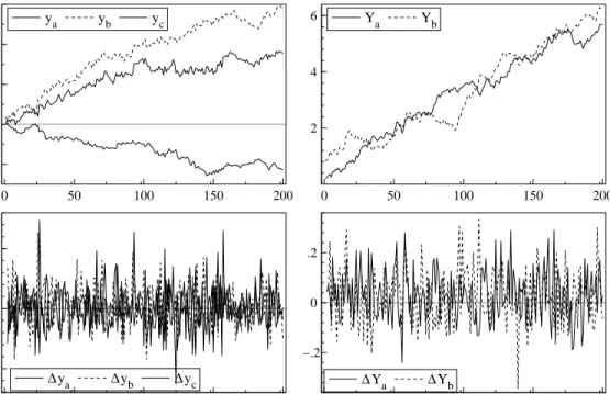
Since I(1) variables ‘wander’ (often quite widely) because of their stochastic trends, whereas (weakly) stationary variables have constant means and variances, if there exists a linear combination that delivers anI(0)relation, it might be thought that it would be obvious from graphs of the variables. Unfortunately, that need not be the case, as figure 1 shows. In panel a, three variables (denotedya,yb,
yc) are plotted that are actually very strongly cointegrated, whereas panel b plots another two (denoted
Ya,Yb) that are neither cointegrated, nor linked in any causal way. Panels c and d respectively show the changes in these variables. It is not obvious from the graphs that the first set are closely linked whereas the second are not connected at all. Nevertheless, the PcGive cointegration test, described in Hendry and Juselius (2000), applied to simple dynamic models relatingya toyb andyc, and YatoYb,
respect-ively takes the values tur = −6.25∗∗ and tur = −2.31, so the first strongly rejects a unit root in the relation, whereas the second does not. Thus, cointegration may or may not exist between variables that do or do not ‘look cointegrated’, and the only way to find out is through a careful statistical analysis, rather than rely on visual inspection. These two points, namely the importance but non-obvious nature of cointegrated relations, motivates our discussion.
The organization of this paper is as follows. Section 2 begins by illustrating the inherently multivari-ate nature of cointegration analysis: several variables must be involved, and this determines the form of the statistical tools required. Section 3 then discusses the conditions under which a vector autore-gressive process (VAR) would provide a feasible empirical model for integrated economic time series, spelling out both its statistical and economic requirements, illustrated by the empirical example used in
1Notice that differencing is not an operator for equations: one can difference data (to create∆x
t), but attempting to difference equation (1) would lead to∆xt= ∆xt−1+ ∆t. Such an equation is not well defined, since∆can be cancelled on both sides, so is redundant.
0 50 100 150 200 −2.5 0 2.5 5 7.5 ya yb yc 0 50 100 150 200 2 4 6 Ya Yb 0 50 100 150 200 −.5 0 .5
∆ya ∆yb ∆yc
0 50 100 150 200
−.2 0 .2
∆Ya ∆Yb
Figure 1 Cointegrated and non-cointegrated time series.
Hendry and Juselius (2000). In section 4, we consider alternative representations of the VAR that yield different insights into its properties under stationarity, and also set the scene for deriving the necessary and sufficient conditions that deliver an integrated-cointegrated process. The purpose of section 5 is to define cointegration via restrictions on the VAR model, and relate the properties of the vector process to stochastic trends and stationary components based on the moving-average representation. Section 6 considers the key role of deterministic terms (like constants and trends) in cointegration analyses.
At that stage, the formalization of the model and analysis of its properties are complete, so we turn to issues of estimation (section 7) and inference (section 8), illustrated empirically in section 9. Section 10 considers the identification of the cointegration parameters, and hypothesis tests thereon, and section 11 discusses issues that arise in the analysis of partial systems (conditional on a subset of the variables) and the closely related concept of exogeneity. Finally, we discuss forecasting in cointegrated systems (section 12) and the associated topic of parameter constancy (section 13), also relevant to any policy applications of cointegrated systems. Section 14 concludes. The paper uses matrix algebra extensively to explain the main ideas, so we adopt the following notation: face capital letters for matrices, bold-face lower case for vectors, normal case for variables and coefficients, and Greek letters for parameters. We generally assume all variables are in logs, which transformation produces more homogeneous series for inherently-positive variables (see e.g., Hendry, 1995a, ch. 2), but we will not distinguish explicitly between logs and the original units.2
2If a variable had a unit root in its original units of measurement, it would become essentially deterministic over time if it had a constant error variance. Thus, absolute levels must have heteroscedastic errors to make sense; but if so, that is not a sensible place to start modeling. Moreover, if the log had a unit root, then the original must be explosive. Many economic variables seem to have that property, appearing to show quadratic trends in absolute levels.
2 The multivariate nature of cointegration analysis
Cointegration analysis is inherently multivariate, as a single time series cannot be cointegrated. Con-sequently, consider a set of integrated variables, such as gasoline prices at different locations as in Hendry and Juselius (2000), where each individual gasoline price (denoted pi,t) isI(1), but follows a
common long-run path, affected by the world price of oil (po,t). Cointegration between the gasoline prices could arise, for example, if the price differentials between any two locations were stationary. However, cointegration as such does not say anything about the direction of causality. For example, one of the locations could be a price leader and the others price followers; or, alternatively, none of the locations might be more important than the others. In the first case, the price of the leading location would be driving the prices of the other locations (be ‘exogenous’ to the other prices) and cointegration could be analyzed from the equations for the other ‘adjusting’ prices, given the price of the leader. In the second case, all prices would be ‘equilibrium adjusting’ and, hence, all equations would contain in-formation about the cointegration relationships. In the bivariate analysis in Hendry and Juselius (2000), cointegration was found in a single-equation model ofp1,t givenp2,t, thereby assuming thatp2,twas a price leader. If this assumption was incorrect, then the estimates of the cointegration relation would be inefficient, and could be seriously biased. To find out which variables adjust, and which do not adjust, to the long-run cointegration relations, an analysis of the full system of equations is required, as illustrated in Section 11.
Here, we will focus on a vector autoregression (VAR) as a description of the system to be investig-ated. In a VAR, each variable is ‘explained’ by its own lagged values, and the lagged values of all other variables in the system. To see which questions can be asked within a cointegrated VAR, we postulate a trivariate VAR model for the two gasoline prices p1,t and p2,t, together with the price of crude oil,
po,t. We restrict the analysis to one lagged change for simplicity, and allow for 2 cointegration relations. Then the system can be written as:
∆p1,t ∆p2,t ∆po,t = φ11 φ12 φ13 φ21 φ22 φ23 φ31 φ32 φ33 ∆p1,t−1 ∆p2,t−1 ∆po,t−1 + α11 α12 α21 α22 α31 α32 ((p1−p2)t−1 p2−po)t−1 ! + ψ1 ψ2 ψ3 d1,t+ π1 π2 π3 + 1,t 2,t 3,t , (2)
wheretis assumed IN3[0,Ω], andΩ is the (positive-definite, symmetric) covariance matrix of the error process.
Within the hypothetical system (2), we could explain the three price changes from period t−1
(previous week) tot(this week) as a result of:
(i) an adjustment to previous price changes, with impactsφij for thejth lagged change in the ith
equation;
(ii) an adjustment to previous disequilibria between prices in different locations, (p1 −p2), and
between the price in location 2 and the price of crude oil,(p2−po), with impactsαi1 and αi2
respectively in theithequation;
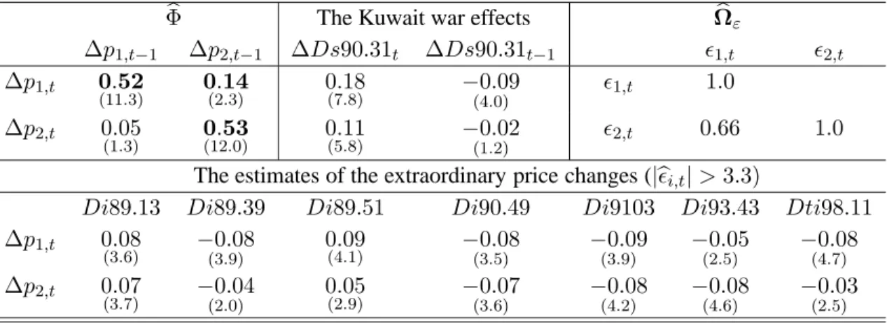
(iii) an extraordinary intervention in the whole market, such as the outbreak of the Kuwait war, de-scribed by the intervention dummyd1,t;
(iv) a constant termπ; and (v) random shocks,t.
When all three prices areI(1), whereas(p1,t−p2,t)and(p2,t−po,t)areI(0), then the latter describe
cointegrated relations, i.e., relations that are stationary even when the variables themselves are non-stationary. Cointegration between the prices means that the three prices follow the same long-run trends, which then cancel in the price differentials. This may seem reasonable a priori, but could nevertheless be incorrect empirically: using multivariate cointegration analysis, we can formally test whether such is indeed the case. In general, we write cointegration relations in the form:
β11p1,t+β12p2,t+β13po,t; and β21p1,t+β22p2,t+β32po,t (3) etc., where, in (2), we have normalizedβ11 =β22= 1, and setβ13=β21= 0. Such restrictions cannot be imposed arbitrarily in empirical research, so we will discuss how to test restrictions on cointegration relations in Section 10.
The existence of cointegration by itself does imply which prices ‘equilibrium adjust’ and which do not; nor does it entail whether any adjustment is fast or slow. Information about such features can be provided by the αij coefficients. For example, α31 =α32 = 0,would tell us that there were no feed-back effects onto the price of crude oil from ‘deviant’ price behavior in the gasoline market. In this case, the price of crude oil would influence gasoline prices, but would not be influenced by them. Next, consider, for example, whenα11=−0.6whereasα21 =−0.1.Then, gasoline prices at location 1 adjust more quickly to restore an imbalance between its own price and the price at location 2 than the other way around. Finally, consider α22 = −0.4: then the location-2 price would adjust quite
quickly to changes in the level of crude oil price. In that case, we would be inclined to say that the price of crude oil influenced the price of location 2 which influenced the price at location 1. This would certainly be the case if the covariance matrixΩεwas diagonal, so there were no contemporaneous links:
ifΩεwas not diagonal, revealing cross-correlated residuals, one would have to be careful about ‘causal’ interpretations. The interpretation of the parameter estimates is generally more straightforward when
Ωε is diagonal, but this is seldom the case; price shocks are often correlated, sometimes indicating
an modeled causal link. For example, if a shock to crude-oil prices affects gasoline prices within the same week (say), the correlations between the residuals from the crude-oil equation and the gasoline equations are the result of a current oil-price effect. Another explanation for residual cross-correlation is omitted variables that simultaneously influence several variables in the system.
As already discussed in Hendry and Juselius (2000), the constant terms, πi, can both describe an
intercept in the cointegration relations and linear trends in the variables, and the empirical analysis can be used to estimate both effects. Finally, the random shocks,i,t,are assumed to be serially independent, and homoscedastic. All these, and other issues, will be discussed and illustrated with an empirical example below.
It should now be evident that a cointegrated VAR provides a rich model: theβij coefficients charac-terize long-run relationships between levels of variables; theαij coefficients describe changes that help
restore an equilibrium market position; theφij coefficients describe short-term changes resulting from previous changes in the market – which need not have permanent effects on the levels; we will com-ment on the intercepts in Section 6; and the intervention effects,ψi,describe extraordinary events in the
market, like the Kuwait war. We might, for example, ask whether such an event affected the gasoline prices differently at different locations (i.e., whether ψ1 6=ψ2), and hence, permanently changed the mean of the price differential (p1 −p2): this will be investigated empirically in Section 9.1. First, we
3 The statistical adequacy of a VAR model
To understand when a VAR is an adequate description of reality, it is important to know the limitations as well as the possibilities of that model. The purpose of this section is, therefore, to demonstrate that a VAR model can be a convenient way of summarizing the information given by the autocovariances of the data under certain assumptions about the DGP: see Hendry (1995a) for details. However, the required assumptions may not hold in any given instance, so the first step in any empirical analysis of a VAR is to test if these assumptions are indeed appropriate.
In section 3.1, we first assume that there are p ≥ 2 variables xi,tunder analysis, and that thep -dimensional processxtis stationary, so does not contain any unit roots. We then derive the VAR model under this simplifying assumption. In section 3.2, we discuss an interpretation of the VAR in terms of rational economic behavior, and finally, in section 3.4, we extend the discussion to consider stability and unit-root properties. Notice that unit roots are a restriction of the initial VAR model, so can be tested, but it transpires that the tests are not standardt,Forχ2.
3.1 Stochastic properties
A stationary VAR arises naturally as a model of a data set (x1, . . . ,xT)0 viewed as a sequence of T
realizations from the p-dimensional process {xt}, given the two general simplifying assumptions of
multivariate normality and time-invariant covariances. Derivations of a VAR from a general DGP are described in (e.g.) Hendry (1995a, ch. 9). The resulting VAR could have many lagged variables, but for simplicity of notation, we restrict attention here to the case with 2 lags denoted VAR(2), which suffices to illustrate all the main properties – and problems (the results generalize easily, but lead to more cumbersome notation). We write the simplest VAR(2) as:
xt=π+Π1xt−1+Π2xt−2+t (4) where
t∼INp[0,Ω], (5)
t = 1, . . . , T and the parameters (π,Π1,Π2,Ω)are constant and unrestricted, except for Ω being
positive-definite and symmetric.
Given (4), the conditional mean ofxtis:
E[xt|xt−1,xt−2] =π+Π1xt−1+Π2xt−2 =mt,
say, and the deviation ofxtfrommtdefinest:
xt−mt=t.
Hence, if the assumptions of multivariate normality, time-constant covariances, and truncation at lag2 are correct, then (4):
• is linear in the parameters; • has constant parameters;
• has normally distributed errorst, with:
• (approximate) independence betweentandt−hfor lagsh= 1,2, . . . .
These conditions provide the model builder with testable hypotheses on the assumptions needed to justify the VAR. In economic applications, the multivariate normality assumption is seldom satisfied.
This is potentially a serious problem, since derivations of the VAR from a general DGP rely heavily on multivariate normality, and statistical inference is only valid to the extent that the assumptions of the underlying model are correct. An important question is, therefore, how we should modify the standard VAR model in practice. We would like to preserve its attractiveness as a reasonably tractable description of the basic characteristics of the data, while at the same time, achieving valid inference. Simulation studies have demonstrated that statistical inference is sensitive to the validity of some of the assumptions, such as, parameter non-constancy, serially-correlated residuals and residual skewness, while moderately robust to others, such as excess kurtosis (fat-tailed distributions) and residual heteroscedasticity. Thus, it seems advisable to ensure the first three are valid. Both direct and indirect testing of the assumptions can enhance the success of the empirical application. It is often useful to calculate descriptive statistics combined with a graphical inspection of the residuals as a first check of the adequacy of the VAR model, then undertake formal mis-specification tests of each key assumption (see Doornik and Hendry, 1999, ch. 10: all later references to specific tests are explained there). Once we understand why a model fails to satisfy the assumptions, we can often modify it to end with a ‘well-behaved’ model. Precisely how depends on the application, as will be illustrated in section 3.3 for the gasoline price series discussed in Hendry and Juselius (2000).
3.2 Economic interpretation and estimation
As discussed in Hendry (1995a), the conditional meanmtcan be given an economic interpretation as
the agents’ plans at timet−1given the past information of the process,xt−1,xt−2, etc., denotedX0t−1. TheINdistributional assumption in (5) implies that agents are rational, in the sense that the deviation between the actual outcomextand the planEt−1[xt|X0t−1]is a white-noise innovation, not explicable
by the past of the process. Thus, the VAR model is consistent with economic agents who seek to avoid systematic forecast errors when they plan for timetbased on the information available at timet−1.
By way of contrast, a VAR with autocorrelated residuals would describe agents that do not use all information in the data as efficiently as possible. This is because they could do better by including the systematic variation left in the residuals, thereby improving the accuracy of their expectations about the future. Checking the assumptions of the model, (i.e., checking the white-noise requirement of the residuals, and so on), is not only crucial for correct statistical inference, but also for the economic interpretation of the model as a description of the behavior of rational agents.
To derive a full-information maximum likelihood (FIML) estimator requires an explicit probability formulation of the model. Doing so has the advantage of forcing us to take the statistical assumptions seriously. Assume that we have derived an estimator under the assumption of multivariate normality. We then estimate the model, and find that the residuals are not normally distributed, or that the residual variance is heteroscedastic instead of homoscedastic, or that residuals exhibit significant autocorrelation, etc. The parameter estimates (based on an incorrectly-derived estimator) may not have any meaning, and since we do not know their ‘true’ properties, inference is likely to be hazardous. Therefore, to claim that conclusions are based on FIML inference is to claim that the empirical model is capable of accounting for all the systematic information in the data in a satisfactory way.
Although the derivation of a FIML estimator subject to parameter restrictions can be complicated, this is not so when the parameters(π,Π1,Π2,Ω)of the VAR model (4) are unrestricted. In that case,
the ordinary least squares (OLS) estimator is equivalent to FIML. After the model has been estimated by OLS, theINdistributional assumption can be checked against the data using the residualsbt.As already mentioned, the white-noise assumption is often rejected for a first tentatively-estimated model, and one has to modify the specification of the VAR model accordingly. This can be done, for example, by:
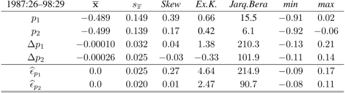
1987:26–98:29 x sx Skew Ex.K. Jarq.Bera min max p1 −0.489 0.149 0.39 0.66 15.5 −0.91 0.02 p2 −0.499 0.139 0.17 0.42 6.1 −0.92 −0.06 ∆p1 −0.00010 0.032 0.04 1.38 210.3 −0.13 0.21 ∆p2 −0.00026 0.025 −0.03 −0.33 101.9 −0.11 0.14 b p1 0.0 0.025 0.27 4.64 214.9 −0.09 0.17 b p2 0.0 0.020 0.01 2.47 90.7 −0.08 0.11
Table 1 Descriptive statistics.
• investigating parameter constancy (e.g., ‘is there a structural shift in the model parameters’?); • increasing the information set by adding new variables;
• increasing the lag length; • changing the sample period;
• adding intervention dummies to account for significant political or institutional events; • conditioning on weakly-exogenous variables;
• checking the adequacy of the measurements of the chosen variables.
Any or all of these steps may be needed, but we stress the importance of checking that the initial VAR is ‘congruent’ with the data evidence before proceeding with empirical analysis.
3.3 A tentatively-estimated VAR
As a first step in the analysis, the unrestricted VAR(2) model, with a constant term and without dummy variables, was estimated by OLS for the two gasoline prices at different locations. Table 1 reports some descriptive statistics for the logs of the variables in levels, differences, and for the residuals. As discussed in Hendry (1995a), since the gasoline prices are apparently non-stationary, the empirical density is not normal, but instead bimodal. The price changes on the other hand, seem to be stationary around a constant mean. From Table 1, the mean is not significantly different from zero for either price change. Normality is tested with the Jarque–Bera test, distributed asχ2(2)under the null, so is strongly rejected for both series of price changes and the VAR residuals. Since rejection could be due to either excess kurtosis (the normal has kurtosis of 3), or skewness, we report these statistics separately in Table 1. It appears that excess kurtosis is violated for both equations, but that forp1,t also seems to be skewed to the right.
The graphs (in logs) of the two gasoline prices are shown in Figure 2 in levels and differences (with 99% confidence bands), as well as the residuals (similarly with 99% confidence bands). There seem to be some outlier observations (larger than±3bσ), both in the differenced prices and in the residuals. The largest is at 1990:31, the week of the outbreak of the Kuwait war. This is clearly not a ‘normal’ observation, but must be adequately accounted for in the specification of the VAR model. The remaining large price changes (> ±3σb) can (but need not necessarily) be intervention outliers. It is, however, always advisable to check whether any large changes in the data correspond to some extraordinary events: exactly because they are big, they will influence the estimates with a large weight and, hence, potentially bias the estimates if they are indeed outliers. The role of deterministic components, such as intervention dummies, will be discussed in more detail in Section 6.
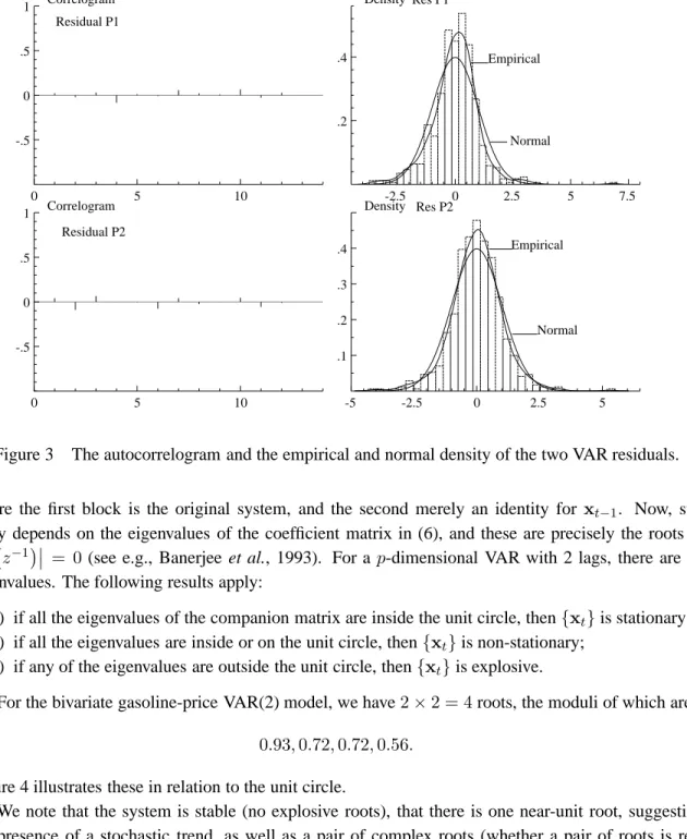
In Figure 3, the autocorrelograms and the empirical densities (with the normal density) are reported for the two VAR residuals. There should be no significant autocorrelation, if the truncation after the
1990 1995 .5 .75 1 Price 1 1990 1995 .5 .75 Price 2 1990 1995 -.1 0 .1 .2 Diff p1 1990 1995 -.1 0 .1 Diff p2 1990 1995 0 .1 .2 Residual 1 1990 1995 0 .1 Residual 2
Figure 2 Graphs of gasoline prices 1 and 2 in levels and differences, with residuals from a VAR(2) and 99% confidence bands.
second lag is appropriate. Since all the autocorrelation coefficients are very small, this seems to be the case. Furthermore, the empirical density should not deviate too much from the normal density; and the residuals should be homoscedastic, so have similar variances over time. The empirical densities seem to have longer tails (excess kurtosis) than the normal density, and the Kuwait war outlier sticks out, confirming our previous finding of non-normality.
3.4 Stability and unit-root properties
Up to this point, we have discussed (and estimated) the VAR model as if it were stationary, i.e., without considering unit roots.3 The dynamic stability of the process in (4) can be investigated by calculating the roots of:
Ip−Π1L−Π2L2xt=Π(L)xt,
whereLixt=xt−i.Define the characteristic polynomial:
Π(z) = Ip−Π1z−Π2z2.
The roots of |Π(z)| = 0 contain all necessary information about the stability of the process and, therefore, whether it is stationary or non-stationary. In econometrics, it is more usual to discuss stability in terms of the companion matrix of the system, obtained by stacking the variables such that a first-order system results. Ignoring deterministic terms, we have:
xt xt−1 ! = Π1 Π2 Ip 0 ! xt−1 xt−2 ! + t 0 ! , (6)
3One can always estimate the unrestricted VAR with OLS, but if there are unit roots in the data, some inferences are no longer standard, as discussed in Hendry and Juselius (2000).
0 5 10 -.5 0 .5 1 Correlogram Residual P1 -2.5 0 2.5 5 7.5 .2 .4 Density Normal Empirical Res P1 0 5 10 -.5 0 .5 1 Correlogram Residual P2 -5 -2.5 0 2.5 5 .1 .2 .3 .4 Density Empirical Normal Res P2
Figure 3 The autocorrelogram and the empirical and normal density of the two VAR residuals.
where the first block is the original system, and the second merely an identity for xt−1. Now, sta-bility depends on the eigenvalues of the coefficient matrix in (6), and these are precisely the roots of Π z−1 = 0(see e.g., Banerjee et al., 1993). For a p-dimensional VAR with 2 lags, there are 2p
eigenvalues. The following results apply:
(a) if all the eigenvalues of the companion matrix are inside the unit circle, then{xt}is stationary; (b) if all the eigenvalues are inside or on the unit circle, then{xt}is non-stationary;
(c) if any of the eigenvalues are outside the unit circle, then{xt}is explosive.
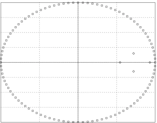
For the bivariate gasoline-price VAR(2) model, we have2×2 = 4roots, the moduli of which are: 0.93,0.72,0.72,0.56.
Figure 4 illustrates these in relation to the unit circle.
We note that the system is stable (no explosive roots), that there is one near-unit root, suggesting the presence of a stochastic trend, as well as a pair of complex roots (whether a pair of roots is real or complex can depend on the third or smaller digits of the estimated coefficients, so is not usually a fundamental property of such a figure). Since there is only one root close to unity for the two variables, the series seem non-stationary and possibly cointegrated.
When there are unit roots in the model, it is convenient to reformulate the VAR into an equilibrium-correction model (EqCM). The next section discusses different ways of formulating such models.
4 Different representations of the VAR
The purpose of this section is to demonstrate that the unrestricted VAR can be given different para-metrizations without imposing any binding restrictions on the parameters of the model (i.e., without
The eigenvalues of the companion matrix
-1.0 -0.5 0.0 0.5 1.0 -1.00 -0.75 -0.50 -0.25 0.00 0.25 0.50 0.75 1.00Figure 4 The roots of the characteristic polynomial for the VAR(2) model.
changing the value of the likelihood function). At this stage, we do not need to specify the order of in-tegration ofxt: as long as the parameters(π,Π1,Π2,Ω)are unrestricted, OLS can be used to estimate them, as discussed in the previous section. Thus, any of the four parameterizations below, namely (4), (7), (8), or (9) can be used to obtain the first unrestricted estimates of the VAR. Although the parameters differ in the four representations, each of them explains exactly as much of the variation inxt.
The first reformulation of (4) is into the following equilibrium-correction form:
∆xt=Φ1∆xt−1−Πxt−1+π+t, (7)
wheret∼INp[0,Ω], with the lagged levels matrixΠ=Ip−Π1−Π2 andΦ1 =−Π2.4 In (7), the
lagged levels matrix,Π, has been placed at timet−1, but could be chosen at any feasible lag without changing the likelihood. For example, placing theΠmatrix at lag2yields the next parameterization:
∆xt=Φ∗1∆xt−1−Πxt−2+π+t (8) whereΦ∗1 = (Π1−Ip),with an unchangedΠmatrix.5 In a sense, (7) is more appropriate if one wants to discriminate between the short-run adjustment effects to the long-run relations (in levels), and the effects of changes in the lagged differences (the transitory effects). The estimated coefficients and their
p-values can vary considerably between the two formulations (7) and (8), despite their being identical in terms of explanatory power, and likelihood (note that they have identical errors{t}). Often, many
4In the general VAR(k) model,Φmatrices cumulate the longer lag coefficients of the levels representation. 5In the general VAR(k),Φ∗matrices cumulate the earlier lag coefficients.
more significant coefficients are obtained with (8) than with (7), illustrating the increased difficulty of interpreting coefficients in dynamic models relative to static regression models: many significant coefficients need not imply high explanatory power, but could result from the parameterization of the model.
The final convenient reformulation of the VAR model is into second-order differences (acceleration rates), changes, and levels:
∆2x
t=Φ∆xt−1−Πxt−1+π+t (9) whereΦ=Φ1−Ip =−Ip−Π2, andΠremains as before. This formulation is most convenient when
xtcontainsI(2) variables, but from an economic point of view it also provides a natural decomposition of economic data which cover periods of rapid change, when acceleration rates (in addition to growth rates) become relevant, and more stable periods, when acceleration rates are zero, but growth rates still matter. It also clarifies that the ‘ultimate’ variable to be explained is∆2xt, which is often treated as a ‘surprise’, but as (9) demonstrates, can be explained by the determinants of the model. Indeed, it can be seen that treating∆2xtpurely as a ‘surprise’ imposes Φ = 0andΠ = 0, and makes the differences behave as random walks.
Although the above reformulations are equivalent in terms of explanatory power, and can be estim-ated by OLS without considering the order of integration, inferences on some the parameters will not be standard unlessxt ∼ I(0).For example, whenxtis non-stationary, the joint significance of the estim-ated coefficients cannot be based on standard F-tests (see Hendry and Juselius, 2000, for a discussion in the context of single-equation models). We will now turn to the issue of non-stationarity in the VAR model.
5 Cointegration in the VAR
We first note that the general condition for xt ∼ I(0) is thatΠhas full rank, so is non-singular. In this case,|Π(1)|=|Π| 6= 0,which corresponds to condition (a) in Section 3.4 that all the eigenvalues should lie within the unit circle. Stationarity can be seen as follows: stationary variables cannot grow systematically over time (that would violate the constant-mean requirement), so ifxt ∼ I(0) in (7), thenE[∆xt] =0. Taking expectations yields:
−ΠE[xt−1] +π=0 (10)
so when Π has full rank, E[xt] = Π−1π. Thus, the levels of stationary variables have a unique equilibrium mean – this is precisely why stationarity is so unreasonable for economic variables which are usually evolving! WhenΠis not full rank (i.e., whenxtexhibitsI(1)behavior), (10) leaves some of the levels indeterminate. At the other extreme, whereΠ=0, the VAR becomes one in the differences ∆xt, and these are stationary ifΦ1−Ip has full rank, in which casext ∼ I(1). Notice thatΦ1 = Ip
whenΠ=0makes∆xta vector of random walks, soxt∼I(2).
Section 5.1 presents the conditions for cointegration in theI(1)model as restrictions on theΠmatrix and Section 5.2 discusses the properties of the vector process when the data areI(1)and cointegrated, based on the moving-average representation.
5.1 Determining cointegration in the VAR model
As discussed in Section 3.4, when some of the roots of the system (4) are on the unit circle (case (b)), the vector process xt is non-stationary. However, some linear combinations, denotedβ0xt,might be
stationary even though the variables themselves are non-stationary. Then the variables are cointegrated fromI(1), down one step toI(0), which Engle and Granger (1987) expressed as being CI(1,1).There are two general conditions forxt∼ I(1), which we now discuss.
The first condition, needed to ensure that the data are notI(0), is thatΠhas reduced rankr < p, so can be written as:
Π=−αβ0 (11)
whereαand βarep×r matrices, both of rankr. Substituting (11) into (9) delivers the cointegrated VAR model:
∆2xt=Φ∆xt−1+α β0xt−1+π+t. (12) An important feature of ‘reduced rank’ matrices likeαandβis that they have orthogonal complements, which we denote byα⊥andβ⊥: i.e.,α⊥andβ⊥arep×(p−r)matrices orthogonal toαandβ(so
α0
⊥α=0andβ0⊥β=0), where thep×pmatrices(α α⊥)and(β β⊥)both have full rankp. These orthogonal matrices play a crucial role in understanding the relationship between cointegration and ‘common trends’ as we explain below (a simple algorithm for constructingα⊥andβ⊥fromαandβis given in Hendry and Doornik, 1996). Note that multiplying (12) byα0⊥will eliminate the cointegrating relations sinceα0⊥α=0.
The second condition, which is needed to ensure that the data are notI(2), is somewhat more tech-nical, and requires that a transformation ofΦin (12) must be of full rank.6 Here, we will disregard the
I(2) problem and only discuss the case when the footnoted condition is satisfied.
Ifr=p, thenxtis stationary, so standard inference (based ont,F,andχ2)applies. Ifr = 0, then ∆xtis stationary, but it is not possible to obtain stationary relations between the levels of the variables by linear combinations. Such variables do not have any cointegration relations, and hence, cannot move together in the long run. In this case, each of (7)–(9) becomes a VAR model in differences but, since ∆xt∼ I(0), standard inference still applies. Ifp > r > 0, thenxt∼ I(1)and there existrdirections in which the process can be made stationary by linear combinations,β0xt. These are the cointegrating
relations, exemplified in (2) above by the two price differentials.
5.2 The VAR model in moving-average form
When the characteristic polynomial Π(z) = Ip −Π1z−Π2z2 contains a unit root, the determinant |Π(z)| = 0 forz = 1, soΠ(z)cannot be inverted to expressxt as a moving average of current and pastt. Instead, we must decompose the characteristic polynomial into a unit-root part and a stationary invertible part, written as the product:
Π(z) = (1−z)Π∗(z),
whereΠ∗(z)has no unit roots, and is invertible. The VAR model can now be written as:
(1−L)xt= ∆xt= [Π∗(L)]−1t. (14) Thus, ∆xt is a moving average of current and past t. To see the nature of that relation, expand [Π∗(L)]−1as a power series inL:
[Π∗(L)]−1=C0+C1L+C2L2+. . .=C(L) (say).
6Specifically:
α0
⊥Φβ⊥=ζη0 (13)
whereζandηare(p−r)×smatrices fors=p−r, which is the number of ‘common stochastic trends’ of first order when xt ∼ I(1). Thus, (13) must have full rank (s =p−r) forxt ∼I(1). Ifs < p−r, then the model containsp−r−s second-order stochastic trends, andxt∼I(2).
In turn, expressC(L)as:
C(L) =C+C∗(L)(1−L),
soC(1) =CasC∗(1)(1−1) =0. We can now rewrite (14) as: ∆xt= [C+C∗(L)(1−L)]t.
By integration (dividing by the difference operator,(1−L)):
xt=C t 1−L +C∗(L)t+x0,
for some initial condition denotedx0, we can expressxtas:
xt=C t
X
i=1
i+C∗(L)t+x0. (15)
In (15), xt is decomposed into a stochastic trend,CPti=1i,and a stationary stochastic component,
et =C∗(L)t.7 There are (p−r)linear combinations between the cumulated residuals,α0⊥Pti=1bi
which define the common stochastic trends that affect the variables xt with weights B, where C = Bα0⊥. In this sense, there exists a beautiful duality between cointegration and common trends. The following example illustrates.
Assume that there exists one common trend between the two gasoline price series, and hence one cointegration relation as reported in Hendry and Juselius (2000). Then,r = 1andp−r = 1, and we can write the moving-average (common-trends) representation as:
p1,t p2,t ! = b11 b21 ! t X i=1 ui ! + δ1 δ2 ! t+ e1,t e2,t ! , (17)
whereB0 = (b11, b21)are the weights of the estimated common trend given byubi =α0⊥bi,andδ1, δ2
are the coefficients of linear deterministic trends inp1,t, p2,t,respectively. Hendry and Juselius (2000) showed that (p1,t −p2,t) ∼ I(0), i.e., that the two prices were cointegrated withβ0 = (1,−1). Fur-thermore, the assumption behind the single-equation model in Hendry and Juselius (2000) was that
α0 = (∗,0).These estimates of β and α correspond to B0 = (1,1) and α0
⊥ = (0,1) in (17). We
express this outcome as: cumulated shocks top2,t give an estimate of the common stochastic trend in this small system. Both prices are similarly affected by the stochastic trend, so that in:
(p1,t−p2,t) = (b11−b21) t
X
i=1
ui+ (δ1−δ2)t+ (e1,t−e2,t) (18)
we have(b11−b21) = 0, and the linear relation (p1,t−p2,t)has no stochastic trend left, thereby defining a cointegration relation.
Note that (17) also allows for a deterministic linear trendtinxt.If, in addition,δ1 =δ2,then both
the stochastic and the linear trend will cancel in the linear relation (p1,t−p2,t)in (18). Ifδ1 6=δ2,then we need to allow for a linear trend in the cointegration relation, such that (p1,t−p2,t−d1t)contains neither
stochastic nor deterministic trends. In this case, we say that the price differential is trend stationary, and that there is a trend in the cointegration space. We have reached the stage where we need a more complete discussion of the key role played by deterministic terms in cointegrated models.
7It can be shown that:
C=β⊥(α0⊥Φβ⊥)−1α0⊥, (16)
so theCmatrix is directly related to (13), and can be calculated from estimates ofα,β,andΦ: see e.g., Johansen (1992a). LettingB=β⊥(α0⊥Φβ⊥)−1,thenC=Bα0⊥,so the common stochastic trends have a reduced-rank representation similar to the stationary cointegration relations.
6 Deterministic components in a cointegrated VAR
A characteristic feature of the equilibrium-correction formulation (12) is the inclusion of both differ-ences and levels in the same model, allowing us to investigate both short-run and long-run effects in the data. As discussed in Hendry and Juselius (2000), however, the interpretation of the coefficients in terms of dynamic effects is difficult. This is also true for the trend and the constant term,as well as other deterministic terms like dummy variables. The following treatment starts from the discussion of the dual role of the constant term and the trend in the dynamic regression model in Hendry and Juselius (2000), and extends the results to the cointegrated VAR model.
When two (or more) variables share the same stochastic and deterministic trends, it is possible to find a linear combination that cancels both the trends. The resulting cointegration relation is not trending, even if the variables by themselves are. In the cointegrated VAR model, this case can be accounted for by including a trend in the cointegration space. In other cases, a linear combination of variables removes the stochastic trend(s), but not the deterministic trend, so we again need to allow for a linear trend in the cointegration space. Similar arguments can be used for an intervention dummy: the intervention might have influenced several variables similarly, such that the intervention effect cancels in a linear combination of them, and no dummy is needed. Alternatively, if an intervention only affects a subset of the variables (or several, but asymmetrically), the effect will not disappear in the cointegration relation, so we need to include an intervention dummy.
These are only a few examples showing that the role of the deterministic and stochastic components in the cointegrated VAR is quite complicated. However, it is important to understand their role in the model, partly because one can obtain misleading (biased) parameter estimates if the deterministic components are incorrectly formulated, partly because the asymptotic distributions of the cointegration tests are not invariant to the specifications of these components. Furthermore, the properties of the resulting formulation may prove undesirable for (say) forecasting, by inadvertently retaining unwanted components – such as quadratic trends, as illustrated by Case 1 below. In general, parameter inference, policy simulations, and forecasting are much more sensitive to the specification of the deterministic than the stochastic components of the VAR model. Doornik, Hendry and Nielsen (1998) provide a comprehensive discussion.
6.1 Intercepts in cointegration relations and growth rates
Another important aspect is to decompose the intercept, π, into components that induce growth in the system, and those that capture the means of the cointegration relations.8 Reconsider the VAR represent-ation (7):
∆xt=Φ1∆xt−1+α β0xt−1+π+t (19) where∆xt∼ I(0)andt∼ I(0). To ‘balance’ (19),β0xt−1must beI(0)also. Since thercointegration relationsβ0xt−1 are stationary, each of them has a constant mean. Similarly,∆xtis stationary with a constant mean, which we denote by E[∆xt] = γ, describing a (p×1) vector of growth rates. This
was illustrated in (17) by allowing for linear trends in the two prices with slope coefficientsδ1 andδ2.
Furthermore, letEβ0xt−1 =µdescribe a(r×1)vector of intercepts in the cointegrating relations. We now take expectations in (19):
(Ip−Φ1)γ=αEβ0xt−1+π=αµ+π.
8One of the reasons we assume all the variables are in logs is to avoid the growth rates depending on the levels of the variables.
Consequently, π = (Ip−Φ1)γ−αµ.Note that the constant termπ in the VAR model does indeed
consist of two components: one related to the linear growth rates in the data, and the other related to the mean values of the cointegrating relations (i.e., the intercepts in the long-run relations). This decomposition is similar to the simpler single-equation case discussed in Hendry and Juselius (2000). When the cointegration relations are trend free as in (19):
β0E[∆xt] =E∆β0xt=β0γ=0,
so we can express (19) in mean-deviation form as:
(∆xt−γ) =Φ1(∆xt−1−γ) +α β0xt−1−µ+t. (20) There are two forms of equilibrium correction in (20): that of the growth∆xtin the system to its mean
γ; and of the cointegrating vectorsβ0xt−1 to their meanµ. The two mean values, γ andµ,play an important role in the cointegrated VAR model, and it is important to ascertain whether they are signific-antly different from zero or not at the outset of the empirical analysis. In the next subsection, we will present five baseline cases describing how the trend and the intercept can enter the VAR specification.
6.2 Five cases for trends and intercepts
The basic ideas are illustrated using thep-dimensional cointegrated VAR with a constant and a linear trend, but to simplify notations we assume that only one lag is needed, soΦ1 = 0. As before, t ∼
INp[0,Ω]:
∆xt=αβ0xt−1+π+δt+t. (21) Without loss of generality, the two(p×1) vectors π and δ can each be decomposed into two new vectors, of which one is related to the mean value of the cointegrating relations, β0xt−1 (case (3) in
section 2 of Hendry and Juselius, 2000), and the other to growth rates in∆xt:
π = αµ+γ0
δ = αρ+τ (22)
Substituting (22) into (21) yields:
∆xt=αβ0xt−1+αµ+γ+αρt+τt+t, (23)
so, collecting terms in (23):
∆xt=α β0:µ:ρ xt−1 1 t + (γ+τt) +t. (24)
Thus, we can rewrite (21) as:
∆xt=α β µ0 ρ0 0 x∗t−1+ (γ+τt) +t, (25)
wherex∗t−1 = (x0t−1,1, t)0. We can always chooseµandρsuch that the equilibrium error(β∗)0x∗t =vt
has mean zero (where β∗ = β0,µ,ρ0), so the trend component in (25) can be interpreted from the equation:
Thus, γ 6= 0 corresponds to constant growth in the variables xt (case 1 in section 2 of Hendry and
Juselius, 2000), whereasτ 6= 0corresponds to linear trends in growth, and so quadratic trends in the variables. Hence, the constant term and the deterministic linear trend play a dual role in the cointegrated model: in theαdirections they describe a linear trend and an intercept in the steady-state relations; in the remaining directions, they describe quadratic and linear trends in the data. To correctly interpret the model, one has to understand the distinction between the part of the deterministic component that ‘belongs’ to the cointegration relations, and the part that ‘belongs’ to the differences.
In empirical work, usually one has some idea whether there are linear deterministic trends in some (or all) of the variables. It might, however, be more difficult to know if they cancel in the cointegrating relations or not. Luckily, we do not need to know beforehand, because the econometric analysis can be used to find out. As discussed below, all these cases can be expressed as linear restrictions on the deterministic components of the VAR model and, hence, can be tested. We now discuss five of the most frequently used models arising from restricting the deterministic components in (21): see Johansen (1994).
Case 1. No restrictions onπand δ, so the trend and intercept are unrestricted in the VAR model. With
unrestricted parameters,π, δ, the model is consistent with linear trends in the differenced series ∆xtas shown in (26) and, thus, quadratic trends inxt. Although quadratic trends may sometimes improve the fit within the sample, forecasting outside the sample is likely to produce implausible results. Be careful with this option: it is preferable to find out what induced the apparent quadratic growth and, if possible, increase the information set of the model. Moreover, as shown in Doornik
et al. (1998), estimation and inference can be unreliable.
Case 2. τ =0,butγ, µ, ρremain unrestricted, so the trend is restricted to lie in the cointegration space, but the constant is unrestricted in the model. Thus,τ being zero in (25) still allows linear, but precludes quadratic, trends in the data. As illustrated in the previous section,E[∆xt] = γ 6= 0
implies linear deterministic trends in the levelxt.When, in addition,ρ6=0, these linear trends in
the variables do not cancel in the cointegrating relations, so the model contains ‘trend-stationary’ relations which can either describe a single trend-stationary variable, (x1,t−b1t) ∼I(0), or an equilibrium relation (β01xt−b2t) ∼ I(0). Therefore, the hypothesis that a variable is
trend-stationary can be tested in this model.
Case 3. δ = 0,so there are no linear trends in (21). Since the constant term π is unrestricted, there
are still linear trends in the data, but no deterministic trends in any cointegration relations. Also, E[∆xt] =γ 6=0,is consistent with linear deterministic trends in the variables but, sinceρ=0,
these trends cancel in the cointegrating relations. It appears from (24) thatπ 6= 0 accounts for both linear trends in the DGP and a non-zero intercept in the cointegration relations.
Case 4. δ = 0, γ = 0, butµ 6=0,so the constant term is restricted to lie in the cointegration space in (25). In this case, there are no linear deterministic trends in the data, consistent withE[∆xt] =0.
The only deterministic components in the model are the intercepts in any cointegrating relations, implying that some equilibrium means are different from zero.
Case 5. δ = 0 and π = 0, so the model excludes all deterministic components in the data, with both
E[∆xt] =0andE[β0xt] = 0,implying no growth and zero intercepts in every cointegrating re-lation. Since an intercept is generally needed to account for the initial level of measurements,x0,
only in the exceptional case when the measurements start from zero, or when the measurements cancel in the cointegrating relations, can the restrictionπ=0be justified.
Turning to our empirical example, Table 1 showed thatE[∆pi,t] = 0could not be rejected. Hence, there is no evidence of linear deterministic trends in the gasoline prices, at least not over the sample
period. The graphs in Figure 1 support this conclusion. We conclude that the cointegrated VAR model should be formulated according to case 4 here, with the constant term restricted to the cointegration space, and no deterministic trend terms.
7 The likelihood-based procedure
So far, we have discussed the formulation of the VAR model in terms of well-specified stochastic and deterministic properties. All this can be done before addressing the unit-root problem. As in Hendry and Juselius (2000), we will now assume that some of the roots of the characteristic polynomial are on the unit circle. This means thatxt∼ I(1), and we consider the cointegrated VAR(2) model (7) where
Π=−αβ0with a constant, a linear trend and a vector of dummy variablesdtincluded:
∆xt=Φ1∆xt−1+αβ0xt−1+π+δt+Ψdt+t. (27) Since∆xt∼I(0)andt∼I(0), all stochastic components in (27) are stationary by definition except for
β0x
t−1.For (27) to be internally consistent, given thatxt∼ I(1),βcannot be a full-rankp×pmatrix
(because then something stationary would be equal to something non-stationary). The only possible solution is thatβis a reduced rank (p×r)matrix withr < p, sorlinear combinations cancel stochastic trends as shown in section 5. Below, we will only discuss the broad ideas of the maximum likelihood estimation procedure, and will not go through the derivations of the results. The interested reader is referred to Johansen (1988, 1995) and Banerjee et al. (1993), inter alia, for details.
The derivation of the maximum likelihood estimator (MLE) is done via the ‘concentrated likeli-hood’ of the VAR model. Since the latter is crucial for understanding both the statistical and economic properties of the VAR, we will demonstrate how it is defined. We use the following shorthand notation:
z0,t = ∆xt
z1,t = xt−1
z2,t = (∆xt−1,1,t,dt).
(additional lagged differences are easily included inz2,t). Rewrite (27) as:
z0,t=αβ0z1,t−1+Θz2,t+t,
whereΘ = (Φ1,π,δ,Ψ).By concentrating out the short-run dynamic adjustment effects, Θz2,t, we are able to obtain a ‘simpler’ model. This is done by first defining the following auxiliary OLS regres-sions:
z0,t = Db01z2,t+ ∆xet
z1,t = Db02z2,t+xet−1,
where∆ext=z0,t−M02M−221z2,t andxet−1=z1,t−M12M−221z2,tare the OLS residuals, andMij =
P
t(zi,tz0j,t)/T is a product-moment matrix, so thatDb01=M02M−221andDb02 =M12M−221. The concentrated model can now be written as:
∆ext=αβ0xet−1+ut, (28)
so we have transformed the original VAR containing short-run adjustments and intervention effects into the ‘baby model’ form, in which the adjustments are exclusively towards the long-run steady-state relations.
The MLE is close to limited-information maximum likelihood (LIML: see Hendry, 1976, for a con-solidation) in that the key issue is to handle a reduced-rank problem, which essentially amounts to
solving an eigenvalue problem. In practice, the estimators are derived in two steps. First, to derive an estimator ofα, assume thatβ is known: thenβ0xet−1 becomes a known variable in (28), soαcan be estimated by OLS. Next, insert thatα =αb(β)in the expression for the concentrated likelihood func-tion, which becomes a function ofβ alone, and no longer depends onα.To find the value of βb that maximizes this likelihood function is a non-linear problem, but one that can be solved by reduced-rank regression (see Johansen, 1988). The solution deliverspeigenvaluesλiwhere0≤λi ≤1:
λ0 = (λ1, λ2, . . . , λp),
which are ordered such that λ1 ≥ λ2 ≥ · · · ≥ λp. The estimate ofβ for r cointegrating vectors is given by thep×r matrix of eigenvectors corresponding to the largestr eigenvalues (the selection of
r is discussed in Section 8). Given the MLEβb ofβ, calculateαb = α(βb). The estimates of the two eigenvectors, and the correspondingαb weights for the empirical example are reported in Table 3.
Eachλi can be interpreted as the squared canonical correlation between linear combinations of the
levels,β0iext−1, and a linear combination of the differences,ϕ0i∆xet. In this sense, the magnitude ofλi
is an indication of how strongly the linear combination β0iext−1is correlated with the stationary part of the processϕ0i∆ext.Ifλi≈0, the linear combinationβ0iext−1 is not at all correlated with the stationary
part of the process, and hence is non-stationary.
In the situation where bothαandβare unrestricted (beyond normalizations), standard errors cannot be obtained, but the imposition of rank and other identifying restrictions usually allows appropriate standard errors to be obtained forαb andβb.
8 Testing cointegration rank
Given that the unrestricted VAR model has been found to satisfactorily describe the data (is a congruent representation), one can start the simplification search, which means imposing valid restrictions on the model such as a reduced-rank restriction, restrictions on the long-run parameters β, and finally restrictions on the short-run adjustment parameters α and Φ. The first, and most crucial, step is to discriminate empirically between zero and non-zero eigenvalues when allowing for sample variation, and then impose an appropriate cointegration rank restrictionron theΠmatrix. Note that:
• if we underestimate r, then empirically-relevant equilibrium-correction mechanisms (EqCMs) will be omitted;
• whereas if we overestimater, the distributions of some statistics will be non-standard, so that incorrect inferences may result from using conventional critical test values (based ont,F,χ2); • forecasts will be less accurate due to incorrectly retainingI(1)components, which will increase
forecast variances.
A test for r cointegrating vectors can be based on the maximum likelihood approach proposed by Johansen (1988). The statistical problem is to derive a test procedure to discriminate between theλi, i=
1, . . . , r, which are large enough to correspond to stationary β0iext−1, and thoseλi, i = r+ 1, . . . , p,
which are small enough to correspond to non-stationary eigenvectors. The rankr is determined by a likelihood-ratio test procedure between the two hypotheses:
Hp: rank=p, i.e., full rank, soxtis stationary;
Hr: rank=r < p, i.e.,rcointegration relations. The test is:
LR(Hr| Hp) =−Tln [(1−λr+1)· · ·(1−λp)] =−T p
X
i=r+1
Ifλr+1 = · · · = λp = 0,the test statistic should be small (close to zero), which delivers the critical
value under the null. The test is based on non-standard asymptotic distributions that have been simulated for the five cases discussed in section 6. There is an additional problem, in thatHr may be correctly accepted whenλr = 0,or evenλr−1 = 0.Therefore, if Hr is accepted, we conclude that there are at
leastp−r unit roots, i.e.,p−r‘common trends’ in the process (but there can be more) corresponding to at mostrstationary relations.
However, if LR(Hr−1|Hp) is calculated, the test statistic includes ln(1−λr), which will not be close to zero, so an outcome in excess of the critical value should be obtained, correctly rejecting the false null of fewer thatrcointegration relations.
As discussed above, the asymptotic distributions depend on whether there is a constant and/or a trend; and whether these are unrestricted or not in the model. However other deterministic components, such as intervention dummies, are also likely to influence the shape of the test distributions. In par-ticular, care should be taken when a deterministic component generates trending behavior in the levels of the data such as an unrestricted shift dummy (· · ·,0,0,0,1,1,1,· · ·): an explanation of the procedure is provided in Johansen, Mosconi and Nielsen (2000), and Juselius (2000): Doornik et al. (1998) also consider the estimation and inference problems resulting from including dummies.
Because the asymptotic distributions for the rank test depend on the deterministic components in the model and on whether these are restricted or unrestricted, the rank and the specification of the deterministic components have to be determined jointly. Nielsen and Rahbek (2000) have demonstrated that a test procedure based on a model formulation that allows a deterministic component, for example a deterministic trend t, to be restricted to the cointegration relations and the differenced component, ∆t= 1, to be unrestricted in the model induces similarity in the test procedure (i.e., the critical values do not depend on the parameter values, so can be tabulated). This is because when there are linear trends in the data, i.e. E[∆xt]6=0,they can enter the model through the constant term,γ 6=0in (26) or through the cointegration relations, ρ 6= 0 in (25). Hence, given linear trends in the data, case 2 is the most general case. When the rank has been determined, it is always possible to test the hypothesis
ρ=0,as a linear restriction on the cointegrating relations.
If, on the other hand,E[∆xt] =0,so there are no linear trends in the data, then the baseline model has the constant term restricted to the cointegration space, which is case 4 above. Therefore, based on the similarity argument, the rank should be based on either case 4 (trends in the data) or case 2 (no trends in the data). Nevertheless, if there is strong prior information that there are trends in the data, but they do not appear in the cointegration relations, then case 3 is the appropriate choice.
9 Empirical model specification
The rank test is defined for a correctly specified model. Prior to the determination of the cointegration rank we should make sure that the empirical model is well-behaved. In Section 9.1, we choose the trend and constant in the baseline model, and account for the extraordinary events in the sample period; whereas in Section 9.2, we discuss the difficult choice of cointegration rank.
9.1 Model specification
For the gasoline example, we found in Table 1 that E[∆xt] = 0 cannot be rejected. Hence, there is little evidence of linear deterministic trends in the data, at least not over the sample period, so we should determine the rank based on a case-4 model. But before testing the rank of theΠmatrix, we need to