Clustering multivariate spatial data based on
local measures of spatial autocorrelation.
An application to the labour market of Umbria. Luca Scrucca
Dipartimento di Economia, Finanza e Statistica Universit`a degli Studi di Perugia, Italy
[email protected] October 17, 2005
Abstract A growing interest in clustering spatial data is emerging in several areas, from local economic development to epidemiology, from remote sensing data to environment analyses. However, methods and procedures to face such problem are still lacking. Local measures of spatial autocorrelation aim at identifying patterns of spatial dependence within the study region. Mapping these measures provide the basic building block for identifying spatial clusters of units. If this may work satisfactorily in the univariate case, most of the real problems have a multidimensional nature. Thus, we need a clustering method based on both the multivariate data information and the spatial distribution of units.
In this paper we propose a procedure for exploring and discover patterns of spatial clustering. We discuss an implementation of the popular partitioning algorithm known as K-means which incorporates the spatial structure of the data through the use of local measures of spatial autocorrelation. An example based on a set of variables related to the labour market of the Italian region Umbria is presented and deeply discussed.
1
Introduction
Suppose we observed the values ofp statistical variables on nareal units of a study region. Such data are referred in the literature aslattice dataand they are character-ized by an arbitrary division of the area being studied into an irregular lattice, often determined by a fixed and countable number of geo-political units with well-defined areal boundaries, such as administrative areas, census tracks, etc. These kinds of data are typically associated with spatial econometrics techniques (Anselin, 1988). However, in other applications the interest lies on studying the absence of spatial randomness of attributes, i.e. the presence ofspatial association which is revealed by a non random pattern of the data values over the study region. Often, spatial association and spatial autocorrelation are used interchangeably to indicate the co-incidence of values similarity with location proximity. Of course, the two concepts
are not identical, the second being a weaker form based on second moments of a joint distribution.
The existence of spatial autocorrelation between neighbouring locations can be assessed globally using popular indicators of spatial autocorrelation (Cliff and Ord, 1981). Recently, the interest has moved to the identification of local patterns of spa-tial association. If global measures can be used to summarize the typical features of spatial autocorrelation for the entire region, local measures of spatial autocorrelation have been proposed for identifying the presence of deviations from global patterns of spatial association, and “hots spots”, such as local clusters or local outliers (Boots, 2002).
Indicators of both global and local spatial association require that the contiguity structure of the spatial units being expressed through the definition of a spatial weights matrix, i.e. an×npositive definite matrix which, in its simplest form, takes on value equal to 1 for neighbouring units and 0 otherwise. Alternative specifications defines units as contiguous if they are within a given distance of each other, or are based on distance decay,k nearest neighbourhood, experts opinions, etc. (Bavaud, 1998).
In a broad sense, local measures of spatial association are part of a larger set of techniques for exploratory spatial data analysis (Unwin, 1996; Unwin and Unwin, 1998). Using visualization tools for spatial data is a natural way to explore the distribution of data values, and these often suggest potentially interesting patterns and hypotheses. In particular, interactive dynamic graphics are a quite useful tool to link the information contained in multivariate spatial data and maps showing the location of spatial units (Buja et al., 1996; Cook et al., 1996; Wilheim and Steck, 1998).
Clustering is a classical theme in the statistical literature and several algorithms have been proposed in the last decades. However, they all deal with the case of independent data, while, according to Tobler’s First Law of Geography1, the main characteristic of spatial data is that the units are correlated. Local measures of spatial autocorrelation, in particular the local Getis-Ord statistic (Getis and Ord, 1992), provide the basis for assessing the presence of spatial clusters. However, these measures are univariate while the data and the real problems we are interested in have often a multidimensional structure. Therefore, an automatic clustering proce-dure which optimize some criterion for the identification of clusters of spatial units based on both their multivariate profiles and their contiguity structure is required.
In Section 2 we will review the main concepts about global and local spatial autocorrelation, together with some of the most popular indicators used to measures them. Examples using socio-economic variables for the Italian region Umbria are also presented. A procedure for the unsupervised classification of spatial data, which takes into consideration also the spatial information during the identification of clusters, is proposed and discussed in Section 3. The following section is dedicated
1“Everything is related to everything else, but near things are more related than distant things” (Tobler, 1979).
to an application of the proposed methodology to the identification of clusters of admnistrative areas in Umbria based on a set of variables expressing the labour market in that region. The final section contains some concluding remarks.
2
Measures of spatial association
Indicate withxi (i= 1, . . . , n) the collected data values for a random variable X on ndata sites in a study region.
The concept of spatial randomness implies that values observed at a given loca-tion do not depend on values observed at neighbouring localoca-tions, i.e. the observed spatial pattern of values is equally likely as any other spatial pattern. We refer to
positive spatial autocorrelationwhen similar values ofxioccurs in the neighbourhood of thei-th data site. On the contrary,negative spatial autocorrelation indicates that neighbouring values ofxi are mutually dissimilar; such dissimilarity is greater than we would expect in case of spatial independence, whose typical configuration is a chessboard pattern.
A spatial autocorrelation index measures the spatial association in the data con-sidering simultaneously both locational and attribute information. There exists two types of indices: global measures, which summarize the spatial association with re-spect to the whole region, and local measures, which refer to the association of a single location with respect to its neighbourhood. In the following subsections we briefly review some popular measures of both global and local spatial association.
2.1 Global spatial autocorrelation
A global measure of spatial autocorrelation is the well-knownMoran’s I given by
I = n n X i=1 n X j=1 wij n X i=1 n X j=1 wijzizj n X i=1 zi2 (1)
wherezi= (xi−x) andwij is a measure of spatial contiguity between the data sites i and j. For row-standardized spatial weights matrix P
i,jwij = n, and equation (1) simplifies to the ratio of spatial crossproducts to deviance. The above index has positive value in case of positive spatial autocorrelation, i.e. when the pairs of deviations from the mean for contiguous locations having the same sign are prevalent. In contrast, when the pairs of deviations from the mean have prevalently opposite sign the index has negative value, therefore showing negative spatial autocorrelation. The observed value ofI can be compared to its distribution under the null hy-pothesis of no spatial autocorrelation, i.e. when the values of xi are independent of the values xj (i6= j) at neighbouring locations. This is equivalent to say that, under the reference null distribution, data are randomly distributed over locations. Either in case of normal distribution of the random variableXor under randomiza-tion sampling, the null distriburandomiza-tion ofI is asymptotically normal and moments, in
particular the expected value and the variance, can be derived (for details see Cliff & Ord, 1981). Therefore, inference can be based on the comparison of the ratio Z(I) = √I−E(I)
Var(I) with quantiles of the standard normal.
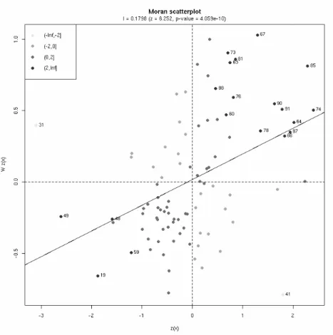
For row-standardized weights matrix the Moran’s statistic can be written in matrix form as I = z>Wz/z>z, which is equivalent to the slope of the regression of the spatially lagged variable Wz on the mean centered variable z. The plot of the constructed variable Wz, which can also be seen as a weighted average of neighbourhood values, versus z is called Moran scatterplot and it provides a nice graphical interpretation to Moran’sI. Such plot can be divided into four quadrants: the top-right and the bottom-left quadrants contain observations showing positive spatial autocorrelation, respectively with high-high and low-low data values. The top-left quadrant contains low values in a neighbourhood of high values (low-high), while the bottom-right quadrant contains high values in a neighbourhood of low values (high-low). In both cases, they are showing spatial outliers.
A different approach to measuring spatial association has been recently proposed by Getis and Ord (1992). Their proposal is based on the definition of a neighbour-hood for each location given by those observations that fall within a critical distance d. The Getis and Ord global spatial association measure is defined as follows:
G= n X i=1 n X j=1 wijxixj n X i=1 n X i=1 xixj (2)
where wij is the (i, j)-th element of a symmetric binary matrix of spatial weights, i.e. wij = 1 for neighbouring locations and 0 elsewhere. The statistic in (2) takes values on [0,1], where values close to 1 indicate clustering of high values, while values close to 0 indicate clustering of low values. Inference for the Getis and OrdG statistic is based on the finding that under a randomization assumption the limiting distribution is normal, so a standardizedz-value can be computed and significance assessed in the usual way (see Getis and Ord, 1992, for details on the derivation of mean and variance under the null hypothesis).
It should be noted that the interpretation ofG is different from that of Moran’s I: the former distinguish the clustering of high and low values, but does not capture the presence of negative spatial correlation; the latter is able to detect both positive and negative spatial correlations, but clustering of high or low values are not distin-guished. Thus, they may be seen as complementary tools, detecting and measuring different aspect of spatial association. Depending on the context, using one or the other can help reveling interesting pattern in the data at hand. For example, if the main goal is to look for clusters in the data theG statistic should be preferred, but if the goal is to detect “hot spots” or spatial outliers then Moran’sI should be used. Example In the present paper we discuss socio-economic data for an Italian region (Umbria). Among the full set of variables, which will be discussed in Section 4, we
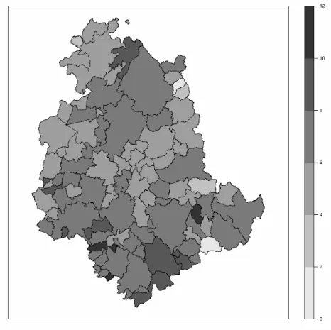
start by analyzing the unemployment rate (%) observed on the year 2001 for the 92 Comuni of Umbria, where a Comune is the smallest administrative area in Italy. The spatial distribution for this variable is shown in the map in Figure 1. Most of the values are in the range 4–8%, with outlying values coming mainly from mountain Comune located in the eastern border. With the exception of Pietralunga in the north east of the region, all the highest rates are in the south part of the region.
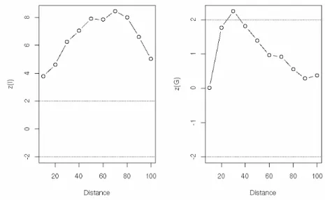
To investigate this aspect we computed the Moran’sI and the Getis-Ord Gfor increasing orders of contiguity. The plots in Figure 2 show the standardized values for the two statistics as a function ofd, the distance between the centroids. Moran’s I is constantly higher than the threshold value (set at 2, roughly the 5% critical value from a standard normal distribution), whileG appears to be significant only ford= 30 km. A more formal procedure would involve the computation of p-values based either on normal approximation or, better, on randomization. However, the conclusions drawn are essentially the same; for example, atd= 30 the p-values based on 999 permutations are 0.001 and 0.027 for, respectively, theI andG statistic.
Figure 1: Spatial distribution of the unemployment rate (%) in Umbria.
2.2 Local spatial autocorrelation
Global measures of spatial association emphasize the average spatial dependence over the study region, hence they will only be useful if spatial dependence is relatively
Figure 2: Standardized global spatial autocorrelation measures as a function of distance (km).
uniform over the study region. If the underlying spatial process is not stationary, global measures may not be representative, particularly if the size of the study region is relatively large. Local measures of spatial association aim at identifying patterns of spatial dependence within the study region (for a review see Boots, 2002). There have been different proposals for local measures, but two in particular are worth mentioning since they are related to the previous global measures of spatial association.
Local Moran’sI was proposed by Anselin (1995) and it is defined as follows:
Ii = zi n X j=1 wijzj n X j=1 zj2/n (3)
for anyi= 1, . . . , n. Large positive Ii values indicate local clustering of data values around the i-th location, similar to that at i and which deviate strongly from the average, either positively or negatively. In contrast, large negative Ii values indi-cate that the sign of data value at thei-th location is the opposite to those of its neighbours.
Local Moran statistic can be used to indicate local instability, i.e. local deviations from global pattern of spatial association, or identify “hot spots”. These are given by significant local clusters in the absence of global autocorrelation, or significant local outliers, i.e. high values surrounded by low ones and vice versa.
The expected value ofIi under the complete randomization assumption is given by
E(Ii) =
−wi (n−1)
and the variance by Var(Ii) = −wi(2)(n−b2) (n−1) + 2wi(kh)(2b2−n) (n−1)(n−2) − w2 i (n−1)2 where b2 = m4/m22 and mr = Pizir/n; wi = Pjwij, wi(2) = P i6=jw2ij and wi(kh)= P k6=i P
h6=iwikwih/2 (Anselin, 1995). However, the distribution ofIiis not asymptotically normal, so its significance is usually based on permutation methods. Under a complete randomization assumption all n data values are permuted, say, B= 999 times, the statistic (3) is computed for each permutation,bIi(b= 1, . . . , B), and thep-value is taken to be approximately equal to #{bIi > Ii}+ 1
B+ 1 . Under the conditional randomization assumption the above scheme is also used, but the value atiis held fixed and the other data values are permuted over the remaining (n−1) data sites.
The local MoranIiis a member of the class of so-called “local indicators of spatial association” (LISA). For Anselin (1995) a LISA statistic must satisfies two require-ments: (a) indicate the extent of significant spatial clustering for each location; (b) the sum of local statistics is proportional to a global indicator of spatial association. There are several LISA forms of global statistics such as local Moran, local Geary, and local Gamma (see Anselin, 1995). The local MoranIi is a LISA statistic since satisfies both requirements: it provides a measure for each data location, and it can be easily shown that, except for a multiplicative factor, the sum of local MoranIis is equal to the global Moran’s statistic in (1).
As for the global measure of spatial association, the Getis and Ord (1992) local indicator is derived using a different approach and it is given by:
Gi = n X j=1 wijxj n X j=1 xj (4)
for any i= 1, . . . , n. This measure is computed as the sum of all the data values in the neighbourhood centered on the i-th location relative to the sum of all data values. In the original proposal, the authors introduced two statistics, Gi and G∗i, where the first does not include the i-th observation in the summations, while the second version does; the formula provided in (4) is their second version, and this one will be used throughout.
Getis and Ord (1992) and Ord and Getis (1995) showed that the Gi statistic is asymptotically normally distributed as the number of neighbours ofiincreases. For not very skewed distributions ofX, a number of 8 neighbours or more is enough to ensure a sufficient approximation. Therefore, inference can be drawn on the basis of standardized scores computed from the following moments:
E(Gi) = wi
Var(Gi) =
wi(n−wi) n2(n−1)
s2 x2
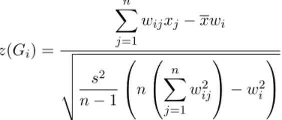
wherewi =Pjwij,x=Pixi/nand s2=Pi(xi−x)2/n. It can be shown that the standardized local Getis-Ord statistic is given by
z(Gi) = n X j=1 wijxj −xwi v u u u t s2 n−1 n n X j=1 w2 ij −w2i (5)
The interpretation ofz(Gi) is straightforward: positive significant values indicate clusters of high values around the i-th location, while negative significant values indicate clusters of low values around thei-th location.
Example (continue) In order to compute the local spatial autocorrelation statis-tics previously reviewed we must define the spatial weights matrixW. For reasons to be discussed in Section 4, we definewij = 1 for any pairs of Comuni whose centroids are within a distance of 30 km, andwij = 0 otherwise.
The standardized Moran’s local statistics for the unemployment rates in Umbria are mapped in Figure 3.
There are Comuni with significant positive values, say withz(Ii)>2, indicating local concentration of high or low values, although we cannot distinguish them based on the Iis. The Moran scatterplot in Figure 4 may help to see that the majority of significant positive cases are in the upper-right quadrant, i.e. they are Comuni with high unemployment rate surrounded by others with high values. Four cases, which appear in the lower-left quadrant, have low values and are surrounded by low unemployment rates (the id number used to identify the Comuni are listed and mapped in the Appendix). The two significant negative values (z(Ii)<−2) indicate the presence of “outliers”: Pietralunga (41) which has a high unemployment rate with neighbouring low values, and Monteleone di Spoleto (31) which has a low value surrounded by high values.
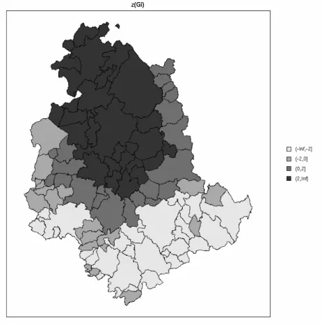
Figure 5 shows the spatial distribution of standardized local Getis-Ord values. Low unemployment rates are more concentrated in the north part of the region, with a cluster of significant low values (z(Gi)<−2) in the eastern part. The two isolated significant values (Pietralunga and Deruta) appear as peaks in spite of having high values since they are surrounded by Comuni of low values. This may seems incorrect, but it is coherent with the definition of theGi statistic, which measures clustering at thei-th location taking into account neighbouring values and excluding the value observed on the i-th site (since wii = 0 by definition). Clearly, significant high unemployment rates (z(Gi)>2) are present in the south part of the region. From this map it is evident the presence of spatial clustering and Figure 5 seems a good starting point for detecting spatial clusters of unemployment rates in Umbria.
Figure 5: Map of standardized local Getis-Ord Gi values for the unemployment rates in
3
Identifying spatial clusters based on local statistics
for spatial autocorrelation
Clustering is a well-established and long-history field in the statistical literature. It has been also extensively studied on other areas, for instance in machine learning as unsupervised learning. Cluster analysis seeks to find groups structure for objects based on their multivariate profiles. Thus, fundamental to clustering is a measure of similarity (or dissimilarity) of the objects being grouped. However, the definition of similarity for spatial data must take into account also the spatial distribution of local units over the study region.
Given n observations in the p-space spanned by a multivariate set of variables, clustering algorithms seek to assign each observation to one ofK groups or classes. This assignment operation can be characterized as a many to one mapping from observations to clusters, with an encoder functionC, so observation iis mapped to cluster C(i). Different clustering algorithms use different encoder functions chosen on the basis of some optimality criteria. For example, popular clustering methods seek to minimize the total within-cluster dissimilarity.
Most clustering methods can be broadly divided into two classes: partitioning methods, which seek to optimally divide objects into a fixed number of clusters, and hierarchical methods, which produce a nested sequence of clusters. Our proposal belong to the first class of methods since it is an implementation of the popular par-titioning algorithm known asK-means to a suitable set of derived spatial variables. The proposed procedure for clustering spatial data is based on the following algorithm:
1. given a spatial weights matrix W, compute for each variable the standard-ized local Getis-Ord statistics. Let z(Gj(xi)) be the statistic in equation (5) computed for the j-th variable (j = 1, . . . , p) on the i-th unit (i = 1, . . . , n). Collect such values on the matrix Zof dimension (n×p). Each column of Z expresses the local autocorrelation pattern for a variable, while each row ofZ provides the clustering profile around each local units.
2. apply theK-means algorithm to this set of new spatially-constructed variables. This step allows to cluster observations based on their multivariate spatial profiles which contain both location and attribute information.
The K-means clustering method seeks to find the optimal partition which minimizes the following objective function:
W SS = K X k=1 X C(i)=k ||zi−zk||2 (6)
where zi is the i-th row of the matrix Z,zk fork = 1, . . . , K are the cluster centers, and ||x−y||=
q Pp
j=1(xj−yj)2 is the Euclidean distance, a measure of within-cluster dissimilarity.
The algorithm starts with an initial set of centers (z1,z2, . . . ,zK), and alternate between mapping units to the nearest center, and then averaging points within cluster to update centers. The algorithm is quite fast and it is not very sensitive to the chosen initial centers, albeit in some circumstances good starting points may help to obtain stable results in repeated applications of the procedure. On the contrary, choosing the number of clusters in the final configuration is a crucial step.
3. repeat the above step for a grid ofk values and select the final configuration based on the optimal number of clusters suggested by the Gapstatistic. The selection of the optimal number of clusters could be based on R2-type statistic with associated F test (Beale, 1969), or on more descriptive mea-sures such as the average silhouette value (Kaufman and Rousseeuw, 1990). Recently, Hastie et al. (2000) have proposed a widely applicable procedure to select the optimal number of clusters. Their proposal is an extension of the classical R2 statistic, so for a configuration of k clusters is given by the following expression:
R2k= 1−W SSk
T SS
where T SS is the total sum of squares, and W SSk is the minimized within cluster sum of squares in equation (6) forkclusters. The statisticR2k provides the proportion of deviance explained by a configuration ofkclusters. However, it cannot be used in model selection since it is a nondecreasing function of k. Suppose we have computedR2kfor a fixed number kof clusters, and we would like to evaluate if it is greater than the value we should expect from a random configuration of independent observations. Such scenario may be simulated through resampling methods. Let Z∗b be a permuted data matrix, obtained by permuting the elements within each column of Z. For a large number of permutations, say B = 999, we compute R∗k,b2, the statistic obtained from applying the K-means algorithm for k clusters with b = 1, . . . , B permuted data. The Gapfunction is defined as
Gap(k) =R2k−R∗k2 where R∗k2= 1 B B X b=1
R∗k,b2. The optimal number of clusters ˆkis the value which maximize the above function, i.e.
ˆ
k= argkmaxGap(k)
The Gapstatistic is of course linked toR2, but it does not have its drawbacks and it can be effectively used to select the optimal configuration of clusters. Example (continue) For illustrative purposes we apply the proposed procedure to only two socio-economic variables measured for the 92 Comuni of Umbria. In the next section we will discuss the full analysis using all the available variables.
In Section 2.2 we analysed in depth the unemployment rate and we mapped the standardized local Getis-Ord statistics in Figure 5. The same procedure has been repeated for the activity rate, giving the map in Figure 6. There appear two main clustering areas, one with higher activity rates in the north-center part of the region, around Perugia and neighbouring Comuni, and one in the south part, around Terni and Narni, with lower activity rates.
Figure 6: Map of standardized local Getis-OrdGi values for the activity rates in Umbria.
Applying the K-means algorithm to the standardized Gi values in this two-variables case is equivalent to look for clusters in the scatterplot shown in the left panel of Figure 7. From such graph we can see that there are roughly two groups of Comuni: one group in the top-left part of the plot, with Comuni having low z-values for the unemployment rate and high z-values for the activity rate, and one group in the bottom-right part of the plot, showing Comuni with highz-values for the unemployment rate and low z-values for the activity rate. Between these two groups there are Comuni with intermediatez-values.
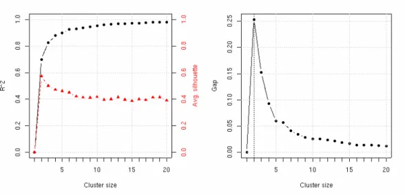
Figure 8 shows some plots used to select the optimal number of clusters: the left plot reports the R2 and the average silhouette value, while the right plot the Gapstatistic. As it can be seen, there is a clear preference for a configuration with k= 2 clusters. The right panel of Figure 7 plots the standardized Gi values for the unemployment and activity rates with points marked by cluster; as expected the
Figure 7: Scatterplot of standardized Gi values for two socio-economic variables. The two
plots are the same except that on the right panel the groups identified by the clustering procedure are marked with different plotting colors and symbols; the points plotted with a + symbol are the within-cluster means.
Figure 8: Graphs of statistics used to select the optimal number of clusters.
clustering procedure has detected the two distinct groups with separation occurring at the intermediate values.
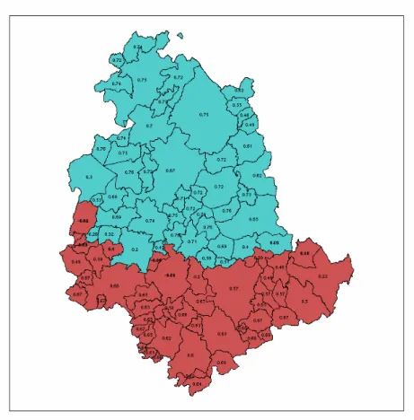
Finally, the spatial distribution of the identified clusters is shown in Figure 9. This map also reports for each Comune the silhouette width, a measure of cluster membership ranging from−1 (for badly classified cases) to 1 (for well classified cases) (Kaufman and Rousseeuw, 1990). Comuni with intermediate values in the scatter-plot of Figure 7 have the lowest silhouette values and are geographically located at the boundary of the two clusters.
Figure 9: Map of clusters identified by theK-means method applied to standardized Gi
values for unemployment and activity rates in Umbria. The value associated with each Comune is the silhouette width, a measure of class membership.
4
Labour market clustering of Umbria Comuni
The clustering method for spatial data discussed in the previous section origi-nated from a research conducted within a project promoted by the Agenzia Umbria Ricerche (AUR), a regional agency for socio-economic researches. The main goal of the project was to detect patterns of regional economic development, an information useful to policy makers for regional planning and development.
In this section we will use a subset of a large set of variables collected from official statistics provided for year 2001 by the Italian official statistical institute (ISTAT). Such variables, broadly referring to the labour market, are reported on Table 1. Umbria, despite being a small region in the center of Italy, is divided into 92 Comuni, with varying geographical extension and population density, mainly due to its morphological aspect, and historically different localization of economic activities.
The first two variables used in the analysis are indicators of labour force offering. Specifically, the unemployment rate (X1) is given by the ratio of unemployed looking
for a job and labour force, while the activity rate (X2) is given by the ratio between
people economically active, i.e. labour force, and the population of 15 years old or more. The remaining variables seek to measure the occupational structure: the quotient of sectoral specialization (X3) is an index of the variability of sectoral
specialization of a territory with respect to the whole region. For thei-th territorial unit is given by X3,i= 1 2 s X j=1 aij ai+ − a+j a++
where aij is the number of employed in sector j on area i, ai+ = Pjaij is the total number of employed on areai, a+j =
P
iaij is the total number of employed on sector j for the whole territory, and a++ = Pi,jaij is the overal number of employed. This index takes value equal to 0 when the occupational structure of the i-th territory is identical to that of the whole region, and it increases approaching the value of 1 as the differences get large. The last two variables (X4 and X5) are
dynamic indicators taken from the local component of a shift-share analysis. These components measure the local contribution to the territorial growth rates from 1991 to 2001, separately, for industrials and services sectors.
Prior to any analysis using spatial data, there is the need to define a spatial weights matrix. Such definition is exogenous to any statistical modeling, and it is typically based on geographic arrangement of the observations or spatial contiguity. In this analysis we adopt a symmetric spatial weights matrix W with wij = 1 if Comuni i and j are within a distance d, and wij = 0 otherwise; by definition wii = 0. The distance between two geographical units is simply defined as the distance between their centroids. Perhaps, some would argue that a better definition should reflect the “economic” distance between two Comuni, which could be based, among others, on travelling time. More investigation is required on this point, albeit our working definition could be considered, at least, a reasonable approximation
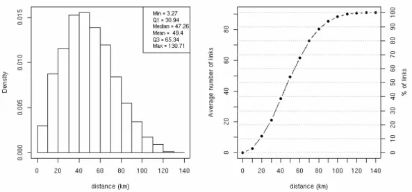
from which to define contiguities. A further point that deserves our attention is the distance within which we define two Comuni as contiguous. From the histogram on the left panel of Figure 10 we see that distances among Comuni of Umbria range from about 3 km up to 130 km, with one quarter of Comuni at a distance of 30 km. For this distance there are 21 links on the average (23%), i.e. each row (column) of W has on average 21 non-zero elements. Thus, in the present analysis the spatial weights matrix was defined for a distance of 30 km between pairs of centroids.
Figure 10: Histogram of distances between Comuni centroids (left panel) and average number (and percentage) of links as function of distance (right panel).
Once we have defined the spatial weights matrix, standardized local Getis-Ord statistics can be computed for each variable in Table 1. The corresponding (92×5) matrixZfilled with such standardized local statistics are then used in the clustering procedure as discussed in Section 3.
The optimal number of clusters chosen on the basis of the Gap statistic is 4, which accounts for almost 80% of total variability, although the average silhoutte width is slightly less than a configuration with 2 clusters (see Figure 11).
Figure 12 shows the map of Umbria with the estimated clusters: a first cluster (numbered as 1 in the map) is given by the Comuni located in the area of Trasimeno lake, Perugia (the chief town of the region), Assisi, and their neighbouring Comuni. A cluster (number 2 in the map) is formed by Spoleto and the closer Comuni of Valnerina, while another cluster (number 4 in the map) is given by the Comuni in the south-west part of the region, with, among others, Terni, Narni, and Orvieto. All these clusters are formed by contiguous Comuni and show a sufficient structure with average silhouette widths equal to 0.45, 0.42, and 0.49. On the contrary, the last cluster (number 3 in the map) contains non-contiguous Comuni, and the structure for this cluster is weak (the average silhouette width is equal to 0.21). However, these territorial units share the characteristic of being geographically located around clusters 1, and acting as a separation area between clusters 1, 2, and 4 (see Figure
Figure 11: Graphs of statistics used to select the optimal number of clusters for the K -means algorithm applied to standardized local Getis-Ord statistics computed for variables in Table 1.
13).
Having defined the clusters geographically it is interesting to note if they share some common characteristics. To this end we can extend what we did in Figure 7, for example, drawing a scatterplot matrix of standardized local Getis-Ord statistics for each variable with cluster identification as marking variable. From such graph (not shown here) it is possible to see some interesting patterns, briefly reported in Table 1.
Table 1: Socio-economic variables used in the spatial clustering procedure. The right part of the table reports for each estimated cluster a stylized interpretation based on the standardized local Getis-Ord values.
Variables Clusters
1 2 3 4
X1 unemployment rate – = = +
X2 activity rate + – = +
X3 quotient of sectoral specialization – + = =
X4 local component of shift-share analysis for industrials
sec-tors
= + = –
X5 local component of shift-share analysis for services sectors + – = –
Legenda:
+ concentration on high values – concentration on low values
= concentration around zero or uniform distribution
Cluster 1 is characterized by a concentration of low values for the unemployment rate and for the quotient of sectoral specialization, but high values of both the
Figure 12: Map of clusters identified by the K-means algorithm applied to standardized local Getis-Ord statistics computed for variables in Table 1.
activity rate and the local growth for services. On the opposite, cluster 2 has high values on the quotient of specialization and industrial local growth, but low values on both the activity rate and the local growth for services. Cluster 4 has high values on both the unemployment and the activity rates, but low values on the local growth components. Finally, the cluster of non-contiguous Comuni (number 3) is characterized by a distribution of values concentrated around zero, except for the local growth of services whose values are almost uniformly distributed over the observed range. Such Comuni have the main characteristic of not showing any clustering of high or low values for any variables considered in the analysis. Hence, their half way position among more clearly defined clusters.
5
Conclusions
The definition of spatial clusters is a main theme on recent economic researches in local and regional development. Other areas, from remote sensing data to epidemi-ology, are interested in identifying spatial clusters of units based on their attributes profile as well as on their spatial distribution. Despite the potential large inter-est, the operational procedures for the identification of such clusters are not well
Figure 13: Silhoutte plot (left panel) and a map of silhouette values (right panel) obtained for the 4-clusters configuration identified by the K-means algorithm applied to spatially derived variables.
developed.
The use of local spatial autocorrelation measures are a first step toward a possible solution to this problem. However, their nature is mainly univariate, while the data and the real problem we are interested in are often multidimensional. At the same time, cluster analysis is a classical theme in the statistical literature, with several algorithms and procedures developed for independent observations. On the contrary, the main characteristic of spatial data is that observations are dependent, and such feature must be incorporated in any sensible method for spatial data clustering.
In this paper we have proposed a procedure for identifying spatial clusters based on both the contiguity structure of units and their attributes information. This procedure is an implementation of the populark-means algorithm for cluster analysis applied to a set of variables expressing local spatial autocorrelations. TheK-means clustering method is connected to mixture models for multivariate normal data. In fact, minimizing the objective function in (6) is equivalent to maximizing the likelihood for a mixture of normals with spherical covariance structure. This suggests that further developments could be based on developping mixture models for more complex structures.
We applied the proposed methodology to a set of variables related to the labour market of Umbria. Results are encouraging, providing a clear picture of main pat-terns in the region with a reasonable economic interpretation of the identified clus-ters.
The procedure can easily be implemented in most statistical packages. For our analysis we use R, a language and environment for statistical computing, freely available under GPL license (R Development Core Team, 2005). Functions which implement spatial clustering procedure are freely available upon request from the author.
References
Anselin L. (1988)Spatial econometrics: methods and models, Kluwer, Dordrecht. Anselin L. (1995) Local indicators of spatial association - LISA,Geographical Anal-ysis,27, 93–115.
Bavaud F. (1998) Models for spatial weights; a systematic look,Geographical anal-ysis,30, 153–171.
Beale, E.M. (1969) Euclidean Cluster Analysis,Boll. ISI, book 2.
Boots, B. (2002) Local measures of spatial association,Ecoscience,9(2), 168–176. Bracalente B. (1991) Analisi di dati spaziali. In Statistica economica, Marbach G. (a cura di), UTET, Torino.
Buja A., Cook D., Swayne D. (1996) Interactive high dimensional data visualization,
Journal of Computational and Graphical Statistics,5(1), 78–99.
Cliff A.D., Ord J.K. (1981) Spatial processes – models and applications, Pion, Lon-don.
Cook D., Majure J.J., Symanzik J., Cressie N. (1996) Dynamic graphics in a gis: ex-ploring and analysing multivariate spatial data using linked software. Computational Statistics,11, 467–480.
Getis A., Ord. J.K. (1992) The analysis of spatial association by use of distance statistics,Geographical Analysis, 24, 189–206, 1992.
Hastie T., Tibshirani R., Eisen M.B., Alizadeh A., Levy R., Staudt L., Chan W.C., Botstein D., Brown P. (2000) ‘Gene shaving’ as a method for identifying distinct sets of genes with similar expression patterns,Genome Biology, 1(2).
Kaufman L., Rousseeuw P.J. (1990) Finding Groups in Data: An Introduction to Cluster Analysis, Wiley, New York.
Ord J.K., Getis A. (1995) Local spatial autocorrelation statistics: distributional issues and an application. Geographical Analysis, 27, 286–306.
R Development Core Team (2005) R: A language and environment for statistical computing. R Foundation for Statistical Computing, Vienna, Austria. ISBN
3-900051-07-0, URLhttp://www.R-project.org.
Tobler W.R. (1979) Cellular geography. In: Philosophy in Geography, Gale S. and Olsson G. (eds.), pp. 379–386. Dordrecht, Holland, D Reidel Publishing Company. Unwin A. (1996) Exploratory spatial analysis and local statistics, Computational Statistics,11, 387–400.
Unwin A., Unwin D. (1998) Exploratory spatial data analysis with local statistics,
The Statistician,47, 415–421.
Wilheim A., Steck R. (1998) Exploring spatial data by using interactive graphics and local statistics,The Statistician,47, 3, 423–430.
Zani S. (1993a) Classificazione di unit`a territoriali e spaziali. In Zani S. (a cura di)
Appendix
Table 2: Table of Umbria Comuni with administrative identification number and id used in Figure 14.
ID Admin.ID Comune ID Admin.ID Comune
PERUGIA 47 54047 SCHEGGINO
1 54001 ASSISI 48 54048 SELLANO
2 54002 BASTIA 49 54049 SIGILLO
3 54003 BETTONA 50 54050 SPELLO
4 54004 BEVAGNA 51 54051 SPOLETO
5 54005 CAMPELLO SUL CLITUNNO 52 54052 TODI
6 54006 CANNARA 53 54053 TORGIANO
7 54007 CASCIA 54 54054 TREVI
8 54008 CASTEL RITALDI 55 54055 TUORO SUL TRASIMENO
9 54009 CASTIGLIONE DEL LAGO 56 54056 UMBERTIDE
10 54010 CERRETO DI SPOLETO 57 54057 VALFABBRICA
11 54011 CITERNA 58 54058 VALLO DI NERA
12 54012 CITTA’ DELLA PIEVE 59 54059 VALTOPINA
13 54013 CITTA’ DI CASTELLO TERNI
14 54014 COLLAZZONE 60 55001 ACQUASPARTA
15 54015 CORCIANO 61 55002 ALLERONA
16 54016 COSTACCIARO 62 55003 ALVIANO
17 54017 DERUTA 63 55004 AMELIA
18 54018 FOLIGNO 64 55005 ARRONE
19 54019 FOSSATO DI VICO 65 55006 ATTIGLIANO
20 54020 FRATTA TODINA 66 55007 BASCHI
21 54021 GIANO DELL’ UMBRIA 67 55008 CALVI DELL’ UMBRIA
22 54022 GUALDO CATTANEO 68 55009 CASTEL GIORGIO
23 54023 GUALDO TADINO 69 55010 CASTEL VISCARDO
24 54024 GUBBIO 70 55011 FABRO
25 54025 LISCIANO NICCONE 71 55012 FERENTILLO
26 54026 MAGIONE 72 55013 FICULLE
27 54027 MARSCIANO 73 55014 GIOVE
28 54028 MASSA MARTANA 74 55015 GUARDEA
29 54029 MONTE CASTELLO DI VIBIO 75 55016 LUGNANO IN TEVERINA
30 54030 MONTEFALCO 76 55017 MONTECASTRILLI
31 54031 MONTELEONE DI SPOLETO 77 55018 MONTECCHIO
32 54032 MONTE SANTA MARIA TIBERINA 78 55019 MONTEFRANCO
33 54033 MONTONE 79 55020 MONTEGABBIONE
34 54034 NOCERA UMBRA 80 55021 MONTELEONE D’ ORVIETO
35 54035 NORCIA 81 55022 NARNI
36 54036 PACIANO 82 55023 ORVIETO
37 54037 PANICALE 83 55024 OTRICOLI
38 54038 PASSIGNANO SUL TRASIMENO 84 55025 PARRANO
39 54039 PERUGIA 85 55026 PENNA IN TEVERINA
40 54040 PIEGARO 86 55027 POLINO
41 54041 PIETRALUNGA 87 55028 PORANO
42 54042 POGGIODOMO 88 55029 SAN GEMINI
43 54043 PRECI 89 55030 SAN VENANZO
44 54044 SAN GIUSTINO 90 55031 STRONCONE
45 54045 SANT’ANATOLIA DI NARCO 91 55032 TERNI