c
AN ENERGY-EFFICIENT P2P PROTOCOL FOR VALIDATING MEASUREMENTS IN WIRELESS SENSOR NETWORKS
BY
VARUN BADRINATH KRISHNA
THESIS
Submitted in partial fulfillment of the requirements
for the degree of Master of Science in Electrical and Computer Engineering in the Graduate College of the
University of Illinois at Urbana-Champaign, 2016
Urbana, Illinois Adviser:
ABSTRACT
Wireless sensor networks (WSNs) should collect accurate measurements to reliably capture the state of the environment that they monitor. However, measurement data collected from one or more sensors may drift or become erroneous due to hardware failures or sensor degra-dation. In WSNs with remote deployments, detecting those measurement errors through a centralized reporting approach can result in a large number of message transmissions, which in turn dramatically decreases the battery life of sensors in the network. In this thesis, we address this issue through three main contributions. First, we propose a protocol in which sensors detect errors in a peer-to-peer (P2P) fashion, and that extends the life of the WSN by minimizing the number of messages transmitted. Second, we propose an effective anomaly detection approach that has low memory and processing requirements, allowing for easy deployment on low-cost sensor hardware. Third, we develop a trace-driven, discrete-event simulator that allows us to evaluate the developed protocol and approach. In doing so, we use three datasets from real WSN deployments, which include indoor air temperature, sea surface water temperature and seismic wave amplitude sensors. Our results show that our P2P protocol can accurately detect errors and simultaneously extend the effective WSN lifetime dramatically compared to the centralized protocol.
ACKNOWLEDGMENTS
I would first like to acknowledge Michael Rausch and Benjamin Ujcich for their contributions to this work. They contributed to the abstract, introduction and related work sections of this thesis. They also helped with improving the quality of the writing. Most importantly, the brainstorming sessions with them produced some of the main ideas in this thesis.
I would like to thank the following people:
• Prof. William Sanders, Dr. Kiryung Lee and Prof. Indranil Gupta for their technical guidance on the project that led to this thesis. Several aspects of the thesis, including writing and organization were improved based on their feedback.
• Prof. Marianne Winslett, Prof. David Yau and Dr. Bimlesh Wadhwa, who recom-mended me for graduate school.
• Prof. Sanders, Prof. Winslett and Prof. Ravishankar Iyer for their continued support of my endeavors.
• Jenny Applequist, James Hutchinson, Aarti Shah, Dr. Wander Wadman, Brett Fed-dersen, and Sangeetha A. J. for their help with proof-reading and improving the writing quality of the thesis.
• My colleagues in the PERFORM Group (Ahmed Fawaz, Atul Bohara, Ben Ujcich, Carmen Cheh, Ken Keefe, Michael Rausch, Mohammad Noureddine, Ronald Wright, and Uttam Thakore) for their support.
• My colleagues in the Information Trust Institute (Prof. David Nicol, Amy Irle, Tim Yardley, Jeremy Jones, Tonia Siuts, Amy Clay, Cheri Soliday, Al Valdes) for their support.
• My former colleagues in the Advanced Digital Sciences Center (Prof. Douglas Jones, Dr. Rui Tan, Dr. Deokwoo Jung, Dr. Binbin Chen, Nguyen Hoang Hai, William Temple, and Ngo Quang Minh Khiem), from whom I have learned a lot.
• The authors of the papers that I have cited in this thesis. They have provided an invaluable knowledgebase.
• My friends and family for their support.
We use three datasets in this study and thank the providers. First, the GeoNet Project in New Zealand for the seismic waveform data [1] (and, in particular, Kevin Fenaughty for his assistance). Second, the TAO Project Office of NOAA/PMEL for the sea water surface temperature data. Finally, the Intel Berkeley Research Lab [2] for the indoor air temperature data.
Finally, I would like to thank the University of Illinois at Urbana-Champaign for providing me with a highly conducive environment for research, access to great people and resources, travel opportunities, and social opportunities.
TABLE OF CONTENTS
LIST OF FIGURES . . . viii
LIST OF ABBREVIATIONS . . . xi CHAPTER 1 INTRODUCTION . . . 1 CHAPTER 2 PRELIMINARIES . . . 4 2.1 System Model . . . 4 2.2 Failure Model . . . 5 2.3 Protocol Requirement . . . 5 2.4 Evaluation Metrics . . . 6
CHAPTER 3 POTENTIAL APPLICATIONS . . . 8
3.1 Indoor Air Temperature of an Office (Berkeley) . . . 8
3.2 Sea Surface Temperatures (TAO) . . . 8
3.3 Seismic Wave Measurement Data (NZ) . . . 12
CHAPTER 4 P2P ERROR DETECTION PROTOCOL . . . 16
4.1 Protocol Description . . . 16
4.2 Required Properties of the Anomaly Detection Approach and Similarity Metric . . . 20
4.3 Memory Requirement . . . 21
4.4 Handling Changes in the Network . . . 21
4.5 Proof of Energy-Optimality . . . 22
4.6 Main Strength and Limitation . . . 25
CHAPTER 5 VALIDATION OF SENSOR MEASUREMENTS . . . 27
5.1 Summary of Approach . . . 27
5.2 Anomaly Detection Approach Assumptions . . . 28
5.3 Isocontours of the Bivariate Normal Distribution . . . 29
5.4 Anomaly Detection Procedure . . . 34
5.5 Similarity Metric . . . 38
5.6 Demonstrating Required Properties of Approach . . . 39
CHAPTER 6 PROTOCOL EVALUATION . . . 48
6.1 Sensor Network Protocol Simulator . . . 48
6.2 Protocol Implementation . . . 51
6.3 Detection Accuracy Results . . . 70
6.4 Reachability Results . . . 70
CHAPTER 7 RELATED WORK . . . 77
CHAPTER 8 CONCLUSION . . . 80
APPENDIX A UNSUITABLE ANOMALY DETECTION APPROACHES . . . 81
A.1 OLS Linear Regression . . . 81
A.2 TLS Linear Regression . . . 83
A.3 Correlation and Dot Products . . . 85
APPENDIX B SENSOR ID AND NAME MAPPING . . . 86
B.1 Berkeley Dataset . . . 86
B.2 TAO Dataset . . . 86
B.3 NZ Dataset . . . 86
LIST OF FIGURES
3.1 Sample of temperature data from Intel Berkeley Research. The white spots
are anomalous measurements. . . 9
3.2 Sample of sea surface temperature data from the Tropical Atmosphere Ocean Project by the Pacific Environmental Laboratory. The white spot in Sensor 2 is an anomaly. . . 9
3.3 TAO Dataset: linear relationships and closeness in measurements values as a function of physical distance. . . 10
3.4 Sample of the seismic waveform data in the GeoNet National Seismograph Network in New Zealand. Note that the seismic amplitude has no unit specified since the data is uncalibrated. . . 12
3.5 NZ Dataset: Anomalies observed in the measurements taken by Sensors 7 and 10. . . 14
3.6 NZ Dataset: Earthquake observed in the measurements taken by three sensors. It is manifested as a spike in the waveform. . . 15
4.1 P2P protocol at each sensor . . . 17
4.2 P2P protocol for Stage 1 (complete stage1) at each sensor . . . 18
4.3 P2P protocol for Stage 2 (complete stage2) at each sensor . . . 19
4.4 P2P Protocol for Stage 3 at sink . . . 20
4.5 WSN showing the routing path of the optimal message in our protocol that reports the erroneous measurement (solid red arrow), unnecessary messages that report anomalous measurements (dashed red arrows), and messages containing measurements (dotted blue arrows). SensorS(1) is faulty. 22 5.1 Single anomalous measurement (in red) in the NZ dataset is detected by constructing an isocontour (blue shaded elliptical region) as a detection boundary. Normal measurements are inside the isocontour and are jointly Gaussian. . . 28
5.2 Anomalies (red crosses) in the NZ dataset due to earthquake observed in normalized measurement space (left) and the space spanned by the two principal components (right). . . 32
5.3 Anomalies (yellow stars) due to the earthquake presented in the seismic waveform in the NZ Dataset (200 sec view). . . 43
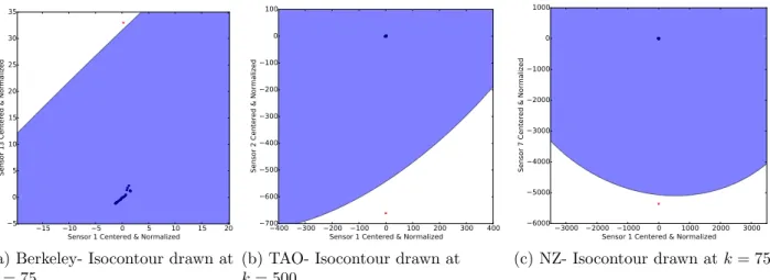
5.4 Anomalies (red crosses) in the three datasets are egregious. They would be detected even if the isocontour were drawn 75, 500 and 3600 standard
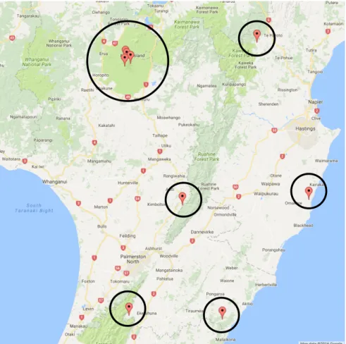
deviations from the mean in the Berkeley, TAO and NZ datasets, respectively. 44 5.5 Map of physical location of select seismic wave sensors in the NZ dataset.
The four sensors grouped in the largest circle are located around a volcano. . 46 6.1 Components of the custom-built discrete event simulator. . . 49 6.2 Centralized validation protocol (Berkeley: Actual Layout): Battery life
illustration for static routing with routing paths shown for 4 arbitrary
sensors. Sink is the star in the center. Crossed-out sensors are unreachable. . 57 6.3 P2P validation protocol (Berkeley: Actual Layout): Battery life
illustra-tion for static routing with routing paths shown for 4 arbitrary sensors.
Sink is the star in the center. Crossed-out sensors are unreachable. . . 58 6.4 Centralized validation protocol (Berkeley: Actual Layout): Battery life
illustration for MBCR routing with routing paths shown for 4 arbitrary
sensors. Sink is the star in the center. Crossed-out sensors are unreachable. . 59 6.5 P2P validation protocol (Berkeley: Actual Layout): Battery life
illustra-tion for MBCR routing with routing paths shown for 4 arbitrary sensors.
Sink is the star in the center. Crossed-out sensors are unreachable. . . 60 6.6 Centralized validation protocol (Berkeley: Grid Layout): Battery life
illus-tration for static routing with routing paths shown for 4 arbitrary sensors.
Sink is near the center. Crossed-out sensors are unreachable. . . 61 6.7 P2P validation protocol (Berkeley: Grid Layout): Battery life illustration
for static routing with routing paths shown for 4 arbitrary sensors. Sink
is near the center. Crossed-out sensors are unreachable. . . 62 6.8 Centralized validation protocol (Berkeley: Grid Layout): Battery life
il-lustration for MBCR routing with routing paths shown for 4 arbitrary
sensors. Sink is near the center. Crossed-out sensors are unreachable. . . 63 6.9 P2P validation protocol (Berkeley: Grid Layout): Battery life illustration
for MBCR routing with routing paths shown for 4 arbitrary sensors. Sink
is near the center. Crossed-out sensors are unreachable. . . 64 6.10 Centralized validation protocol (NZ: Actual Layout): Battery life
illustra-tion for static routing with routing paths shown for 2 arbitrary sensors.
Sink is the star in the ring topology. Crossed-out sensors are unreachable. . . 66 6.11 P2P validation protocol (NZ: Actual Layout): Battery life illustration for
static routing with routing paths shown for 2 arbitrary sensors. Sink is
the star in the ring topology . . . 67 6.12 Centralized validation protocol (NZ: Actual Layout): Battery life
illustra-tion for MBCR routing with routing paths shown for 2 arbitrary sensors.
Sink is the star in the ring topology . . . 68 6.13 P2P validation protocol (NZ: Actual Layout): Battery life illustration for
MBCR routing with routing paths shown for 2 arbitrary sensors. Sink is
6.14 Results for Intel Berkeley Dataset (Actual Layout). The inverse functions of Longevity and Reachability, which are the number of sensors dead and
unreachable, respectively, are plotted. . . 72
6.15 Results for Intel Berkeley Dataset (Grid Layout). The inverse functions of Longevity and Reachability, which are the number of sensors dead and unreachable, respectively, are plotted. . . 73
6.16 Results for TAO Dataset. The inverse functions of Longevity and Reacha-bility, which are the number of sensors dead and unreachable, respectively, are plotted. . . 75
6.17 Results for NZ Dataset. The inverse functions of Longevity and Reacha-bility, which are the number of sensors dead and unreachable, respectively, are plotted. . . 76
A.1 NZ dataset: OLS regression used in anomaly detection. . . 82
A.2 NZ dataset: Failure of OLS regression used in anomaly detection. . . 83
LIST OF ABBREVIATIONS
2-D Two Dimensional
AR Auto-Regressive
ARIMA Auto-Regressive Integrated Moving Average CPU Central Processing Unit
EPIC Explicitly Parallel Instruction Computing MBCR Minimum Battery Cost Routing
NOAA US National Oceanic and Atmospheric Administration
NZ New Zealand
P2P Peer-to-peer
PCA Principal Component Analysis PDF Probability Density Function
PMEL Pacific Marine Environmental Laboratory SST Sea Surface Temperatures
TAO Tropical Atmosphere Ocean Project TPM Trusted Platform Module
US United States
CHAPTER 1
INTRODUCTION
Wireless sensor networks (WSNs) are being increasingly deployed in a number of differ-ent areas, most recdiffer-ently in scenarios involving the Internet of Things (IoT devices). In remote monitoring applications, sensors measure temperature and humidity of forest envi-ronments [3], animal habitats [4], crops [5], etc., and measure vibrations in volcanoes [6] and in civil structures [7], such as bridges [8]. It is essential that those WSNs are designed in a way that minimizes energy consumption of sensors, since the sensors are typically battery-powered. Therefore, extensive research has been performed in designing protocols that extend the lifetime of sensor networks [9].
Measurements from sensors in a WSN may become faulty or drift with time from their true values because of natural degradation of hardware, hardware failures, or manufacturing defects [10]. This can lead to poor measurement quality, which can in turn undermine the monitoring benefits of installing the sensors. There is a need to develop an automated error detection protocol, but the challenge is to minimize its overhead and impact on battery life of individual sensors as well as the connectivity of the network.
Sensor measurement errors manifest themselves as anomalies, and these anomalies need to be reported to the sink (i.e., base station of the sensor network) in a timely fashion, so that the faulty sensors can be investigated. In a naive centralized protocol for validating measurements [10] [11], every sensor periodically reports its measurements to the sink (e.g., via a spanning tree or a DAG topology). The sink then runs a centralized anomaly detec-tion algorithm on these collected measurements, to detect anomalies. While this scheme is attractive in its simplicity, it has two major drawbacks. First, sensors farthest from the sink (by number of hops) may have to route their sensor data through many other sensors to reach the sink. As message transmission consumes significantly more energy than other
sen-sor functions [12], the number of message transmissions should be minimized when possible to extend the sensor network’s life. Second, over a long timeframe, sensors closest to the sink will have more data routed through them on behalf of other sensors farther from the sink. As a result, those sensors closest to the sink will exhaust their battery power and die before sensors farthest from the sink. This disconnects the network earlier, and results in far away sensors needing to transmit at higher amplitudes to reach the sink, further depleting their batteries. Unreachable sensors are effectively “dead” from the sink’s point of view.
In this thesis we adopt a peer-to-peer (P2P) approach for error detection. Such an ap-proach drains the power of sensors in the network more equitably. As a result, sensors closest to the sink can last longer in the P2P approach than in the centralized approach. That al-lows sensors farther from the sink to communicate with the sink for a longer time than possible in the centralized approach. While the usefulness of such a distributed protocol was acknowledged in [6] (in the context of seismic activity monitoring in volcanoes), the authors did not propose an energy-efficient solution.
To the best of our knowledge, ours is the first measurement error detection protocol for WSNs that minimizes the energy cost of transmitting the additional messages required to report measurement errors. The protocol is distributed, and is designed to be widely applica-ble in the context of battery-constrained sensor monitoring, for environments including (but not limited to) indoor spaces, forests, agricultural soil, oceans, volcanoes, distant planets, etc.
Although the P2P protocol reduces the number of message transmissions needed to capture a sensor that is in error, it shifts the onus of anomaly detection from the sink onto the sensors themselves. Therefore, the CPU consumption on sensors increases, and this has an impact on sensor battery life. However, we show that increasing computation costs while decreasing communication costs leads to a net benefit in extending the life of the WSN because communication drains sensor battery faster than computation.
We make three main contributions in designing an energy-efficient protocol to validate sensor measurements. First, we design a P2P error detection protocol that is optimal in that it minimizes message transmissions, thereby extending sensor battery life. Second, we provide a theoretically supported error detection mechanism that has properties required by
the protocol in order to minimize message transmissions. Finally, we evaluate our protocol using a custom-built simulator that uses data traces from two real WSN deployments, as well as real topologies. Our results show that the P2P approach dramatically extends network lifetime.
The thesis is organized as follows. The assumptions within which the protocol is energy-optimal are stated in Chapter 2. The datasets we use to motivate and evaluate our approach are described in Chapter 3. The protocol is described and analyzed in Chapter 4. A val-idation mechanism to support the protocol is presented in Chapter 5. The results of the evaluation of our protocol on the datasets are presented in Chapter 6. Related work is discussed in Chapter 7, and we conclude in Chapter 8.
CHAPTER 2
PRELIMINARIES
In this chapter, we describe our assumptions for the model within which our error detection protocol is energy-optimal with regard to minimizing message transmissions.
2.1
System Model
A WSN comprises a multitude of sensors that use wireless radio communications to transmit, receive, and forward measurements to a base station or sink. Depending on the application, the measurements may be of temperature or humidity of environments, seismic vibrations, etc. Our protocol was designed to be broadly applicable to a range of WSN applications, and is thus agnostic to the application or physical quantities being measured by the sen-sors in the network. We do, however, require that every sensor have at least two other neighboring sensors that can be used for voting on whether that sensor’s measurements are anomalous. The WSN may comprise heterogeneous and multimodal sensors that measure different physical quantities, such as temperature and pressure.
In this thesis, we design the error detection approach for a WSN model in which each sensor has a finite, exhaustible, and non-renewable power supply. That is the case for sensors that rely solely on batteries and do not have access to external power sources (e.g., solar power, or the power grid). Each sensor communicates wirelessly. There are many different wireless communication technologies that a sensor could employ; laser, infrared, and radio frequency (RF) are the most common. We chose to focus on an RF-based system with omnidirectional antennae, which implies that all communication is broadcast to sensors within wireless range. Upon system deployment, there are a multitude of sensors alive in the WSN. The sensors sample and report measurements at discrete time intervals ∆t, whose value is set by the
network administrator depending on the application (e.g., ∆t = 15 s). Between consecutive reports, sensors can go into a low-powered state to reduce battery consumption (see [13]).
2.2
Failure Model
In our model, a sensor is faulty if it reports measurements that statistically deviate sig-nificantly from past measurements, given the same environmental conditions. We refer to measurements that are not erroneous as “proper.” We assume sensors will not intentionally act in a malicious manner, and that Byzantine faults do not occur.
We do not assume a fail-stop model. In the event of a transient error, the network administrator may allow the sensor to continue reporting measurements to the sink. In the event of a persistent error, the sensor may be forced by the network administrator to fall back to a “routing-only mode,” in which it serves as a routing node in a multi-hop network, but does not generate measurement packets itself.
We say that sensors in our model arealive until their batteries are depleted, in which case they are dead. Our P2P protocol operates at the application level of the networking stack, and can run on top of lower-level routing protocols such as SPMS [14] and MBCR [15], or gossip style failure detection protocols such as [16] to detect node failures that occur before battery depletion. Our protocol may be able to run along with the methods in [17], for robustness to message drops or ordering issues, but that is not the focus of this thesis.
2.3
Protocol Requirement
The WSN network administrator requires erroneous measurements to be reported immedi-ately after detection. Since the detection is performed at the sink in the centralized protocol, the sensors mustsynchronously report measurements periodically (at every discrete time in-terval) to the sink for real-time error detection. In the P2P approach, however, sensors exchange readings among themselves synchronously for error detection, but messages are reported to the sinkasynchronously, only when an error is detected. In addition, the sensors
in the P2P approach could report their measurements to the sink in large batches if the net-work administrator needs to keep a record of all measurements at the sink. Such batching prolongs the overall lifetime of the network [18].
The error may be due to a fault or a legitimate rare event in the environment being monitored (such as an earthquake). We believe both events are of interest to the network administrator, and show in Section 5.7 that they can be easily differentiated using appropri-ate detection thresholds. The Hidden Markov Model-driven approach presented in [19] may also be applicable in making that differentiation.
2.4
Evaluation Metrics
Sensors with finite, nonrenewable energy sources will inevitably expend all of their energy and cease to report measurements, so it is important to design protocols that extend the lifetime of the WSN. At start-up, all sensors are alive with full battery power, and as time progresses their battery power gets depleted. The rate at which that depletion happens depends mostly on how much radio and CPU are used by the sensor.
We quantify the lifetime of the entire WSN by defining two metrics from different per-spectives:
Longevity quantifies the WSN’s lifetime from each sensor’s perspective. We define longevity(λ) as the time it takes for λ sensors to die because of battery depletion.
Reachability quantifies the WSN’s lifetime from the sink’s perspective. We define
reachability(ω) as the time it takes before ω sensors lose end-to-end connectivity with the sink (or become unreachable).
Together, longevity and reachability quantify the survivability of the WSN. We say that the validation protocol is energy-efficient if it extends the survivability of the WSN.
In examining the shortcomings of the centralized validation approach, one can see that the survivability of the WSN is constrained by the time it takes for sensors closest to the sink to expend their energy, and the repercussions that has on the reachability of sensors farthest from the sink. Similarly, survivability is constrained in the P2P validation approach, where CPU consumption increases on the sensors, affecting longevity. Because of that trade-off, it
CHAPTER 3
POTENTIAL APPLICATIONS
In this chapter, we use three independent datasets to motivate the applications of our dis-tributed validation protocol. The datasets illustrate the kinds of anomalies seen in measure-ments taken from sensors measuring air temperature of buildings, water temperature of seas and seismic waves on the Earth’s surface.
We use these datasets to evaluate our approach, and refer to them in the thesis by the shorthand given in the parenthesis.
3.1
Indoor Air Temperature of an Office (Berkeley)
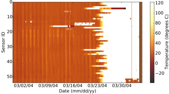
This is a dataset of temperature measurements from 54 Mica2Dot sensors with weather boards deployed at the Intel Berkeley Research Lab [2], in the US. The dataset in its entirety is plotted as a heatmap in Fig. 3.1. The temperatures are nearly all below 30 ◦C, which is normal for an indoor environment. However, it can be clearly seen that sensor 14 (in the 14throw) has reported temperatures of over 120◦C between 2 and 9 March 2004. The sensor
readings proceed to deteriorate and ultimately all become anomalous. These anomalies were present in the dataset despite averaging of measurements in one-hour periods, and are clearly indicative of errors, which are most likely due to battery drain.
3.2
Sea Surface Temperatures (TAO)
This dataset was obtained from the Tropical Atmosphere Ocean Project (TAO) by the Pacific Marine Environmental Laboratory (PMEL), and supported by the US National Oceanic and Atmospheric Administration. We extract-time aligned data from 8 moorings located in the
03/02/04 03/09/04 03/16/04 03/23/04 03/30/04
Date (mm/dd/yy)
0
10
20
30
40
50
Sensor ID
20
0
20
40
60
80
100
120
Temperature (degrees C)
Figure 3.1: Sample of temperature data from Intel Berkeley Research. The white spots are anomalous measurements.
09/01/05 10/01/05 11/01/05 12/01/05 01/01/06
Date (mm/dd/yy)
0
1
2
3
4
5
6
7
Sensor ID
10
5
0
5
10
15
20
25
30
Temperature (degrees C)
Figure 3.2: Sample of sea surface temperature data from the Tropical Atmosphere Ocean Project by the Pacific Environmental Laboratory. The white spot in Sensor 2 is an anomaly.
24.15
24.2
24.25
24.3
24.35
24.4
sst0n125w (
◦C
)
24
25
26
27
28
29
30
31
Ot
he
r s
en
so
rs
(
◦C
)
sst0n140w
sst0n155w
sst0n180w
sst0n165e
Figure 3.3: TAO Dataset: linear relationships and closeness in measurements values as a function of physical distance.
Pacific Ocean on the equator (0◦N) at 95◦W, 110◦W, 125◦W, 140◦W, 155◦W, 170◦W, and 165◦E. Several sensors are located on the moorings, as described in [20], and we analyze the sea water temperature data measured by the thermistors at 1 to 1.5 m below the surface.
The data for all 8 sensors was available between 2 Aug 2005 and 16 Jan 2006, and is illustrated in Fig. 3.2. The anomaly in the dataset is the obvious white mark for Sensor 2. The reason for the anomaly was not described by the providers of the dataset, and we assume that the sensor malfunctioned in those time periods. Note that water temperatures can go below 0 ◦C, but that only happens near the North and South poles, and the temperature never goes below−2◦C. Therefore, the anomalies in this particular dataset could be detected by trivial thresholds set with that prior knowledge.
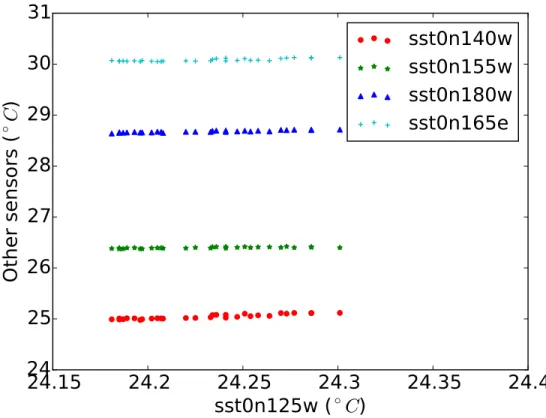
Figure 3.3 shows how linearly related the ocean temperatures seem to be over a five hour period. There are 30 measurements in the plot and it can be seen that the magnitudes of the temperatures bear some relationship to the physical distance between the sensors. Sensor sst0n125w measures temperatures in the range of 24◦C. Among the sensors plotted, Sensor
sst0n140w is the nearest to sst0n125w in distance (it is 15 degrees west of sst0n125w, as measured by longitudinal geodesic distance). It can be seen that the measurements taken by sst0n140w are nearest in magnitude to sst0n125w. The next sensor west of sst0n140w on the equator is sst0n155w, and its magnitude is the next closest to sst0n125w. That trend continues on till sst0n165e, which is farthest (both in geodesic distance and measurement magnitude) to sst0n125w.
The highest resolution data obtained from the sensors was a 10 minute average reading. That data was stored internally in the mooring, and acquired from the memory later when recovering the mooring. Daily averages were transmitted to satellites for what the PMEL refers to as real-time monitoring. We do not know why the more fine-grained information is not transmitted, but we assume it is because of the sensors are battery-powered and the energy cost of transmission is high.
Since the data is monitored once a day, the more fine-grained weather changes cannot be monitored. If anomalous readings were to be recorded, they would not be discovered until the end of the 24 hour cycle (assuming they significantly alter the daily mean). For example, if changes in sea temperature were important to monitor to identify potential cyclones, the necessary granularity would be missing in this data. The TAO project was set up to study the El Nino Southern Oscillations, which can lead to severe cyclones.
In order to capture and report the fine-grained changes in measurements, our energy-efficient P2P validation protocol can be applied in a way that minimizes the transmission cost for the sensors. The protocol can be used to monitor and report anomalies in more fine-grained temporal resolution so that the appropriate actions can be taken (raise an alarm for a storm, or disregard the reading as unreliable). The non-anomalous readings could continue to be recorded once a day, or on recovering the mooring, and are not as important to transmit since they do not contain information that needs to be acted upon immediately. In addition, more spatially fine-grained data can be obtained by installing more moorings in the area, forming a more dense sensor network.
14:00
01/03
01/03
17:00
20:00
01/03
23:00
01/03
02:00
01/04
05:00
01/04
08:00
01/04
01/04
11:00
Time (hrs) and Date (mm/dd)
0
5
10
15
20
25
30
35
40
Sensor ID
50000
40000
30000
20000
10000
0
10000
20000
30000
40000
50000
Seismic Wave Amplitude
Figure 3.4: Sample of the seismic waveform data in the GeoNet National Seismograph Network in New Zealand. Note that the seismic amplitude has no unit specified since the data is uncalibrated.
3.3
Seismic Wave Measurement Data (NZ)
This dataset was obtained from the GeoNet National Seismograph Network in New Zealand [1]. Broadband seismic data was obtained from stations evenly distributed throughout the coun-try.
This dataset is the most interesting of the three that we study in this thesis. That is because the anomalies in this dataset not only correspond to sensor failures, but also are caused by extreme events (an earthquake).
The seismic waveform data we extracted is from 41 stations in the seismograph network, for the 24hr period between 12:00hrs on 3 January and 12:00hrs on 4 January 2016. The sampling rate is 100 samples per second. We take the average of each second and detect anomalies in those averages. As a result, we do not perform anomaly detection at the same rate at which the data is sampled, but at a much lower rate. The lower rate at which we perform anomaly detection is sufficiently high to capture anomalies, and sufficiently
low to ensure that anomalies are reported in a timely manner. The lower rate also helps dramatically minimize computation and network usage related costs. The averaged data is shown as a heat map in Fig. 3.4.
The seismic amplitude has no unit specified since the data is uncalibrated. The providers of the data informed us that calibrating the data is a complex procedure, and we avoided the need for that procedure by normalizing the data in our models so that the normalized values are inherently unitless.
The large white gap for Sensor 7 was due to a failure. That anomaly is illustrated along with another anomaly with Sensor 10 in time series plots in Fig 3.5.
There were other, less noticeable, white spots (most noticeable in Sensor 1, at high zoom) at 00:08 hrs on 4 January, and they coincided with a strong earthquake that had occurred at the same time (with a magnitude of 5.0 on the Richter scale). Based on separate earthquake data provided by GeoNet, we found the ground truth on the earthquake recorded at 00:08 hrs on 4 January. The details of the earthquake are available at http://www.geonet.org. nz/quakes/region/newzealand/2016p008122.
The impact of the earthquake on the seismic waveforms for three seismic stations (closest to the earthquake epicenter) is illustrated in Fig 3.6. The spike due to the earthquake is noticeable in the measurements taken by all the stations in the seismograph network, but to varying degrees. For example, the spike due to the earthquake is less prominent for Sensors 7 and 10, but is still visible in Fig 3.5.
20000
15000
10000
5000
0
5000
10000
Seismic Amplitude
Sensor 10
1.6
1.4
1.2
1.0
0.8
0.6
0.4
0.2
0.0
0.2
Seismic Amplitude
1e7
Sensor 7
14:00
01/03
17:00
01/03
20:00
01/03
23:00
01/03
02:00
01/04
05:00
01/04
08:00
01/04
01/04
11:00
Time/Date in January 2016
10000
5000
0
5000
10000
Seismic Amplitude
Sensor 7 Zoomed-In
Figure 3.5: NZ Dataset: Anomalies observed in the measurements taken by Sensors 7 and 10.
800000
600000
400000
200000
0
200000
400000
600000
800000
1000000
Seismic Amplitude
Sensor 1
80000
60000
40000
20000
0
20000
40000
60000
Seismic Amplitude
Sensor 31
14:00
01/03
17:00
01/03
20:00
01/03
23:00
01/03
02:00
01/04
05:00
01/04
08:00
01/04
01/04
11:00
Time/Date in January 2016
30000
20000
10000
0
10000
20000
30000
Seismic Amplitude
Sensor 19
Figure 3.6: NZ Dataset: Earthquake observed in the measurements taken by three sensors. It is manifested as a spike in the waveform.
CHAPTER 4
P2P ERROR DETECTION PROTOCOL
We propose a P2P sensor measurement error detection protocol as an alternative to the centralized protocol described in Chapter 1, which we use as a comparison baseline. In this section, we describe that protocol and show that it minimizes the number of message transmissions within the assumptions stated in Chapter 2. In that sense, it is energy-optimal.
4.1
Protocol Description
The protocol comprises three stages: reference sensor identification, telemetry/detection, and response. In the first stage, each sensor identifies neighboring sensors whose measurements are most similar to its own, and marks those sensors as reference sensors. The reference sensors are used in the second stage of the protocol, which combines telemetry with error detection and fault reporting. In the third stage, the sink identifies the faulty sensor from fault reports, and responds to the reports.
The main algorithm running on each sensor, which encompasses all three stages, is de-scribed in Fig. 4.1. Note that Stage 2 cannot be started until Stage 1 is completed. Also, note that Stage 3 happens at the sink, and is only reflected in the sensor behavior in lines 17–18 of the algorithm in Fig. 4.1. Stage 3 happens after a fault has been reported in Stage 2, and if a sensor has been commanded to operate in a forwarding-only mode, the sensor remains in that mode, effectively exiting from Stage 2.
Each sensor in the WSN operates independently and its stage does not need to be in sync with other sensors’ stages. For example, sensorS(1) might have just joined the WSN and be in Stage 1, while sensor S(2) is in Stage 3.
using its omnidirectional antenna at all discrete time steps given by the sampling interval. Figure 4.1: P2P protocol at each sensor
1: stage1 complete← False
2: candidates ← empty 1D array(size M)
3: reference sensors ← empty 1D array(size R)
4: candidate measurements ← empty 2D array(size M,size T)
5: in forwarding only mode← False
6: while Truedo
7: neighbor messages ←get messages from buffer()
8: for messagein neighbor messages do
9: if message.id = sink.idand message.command = forwarding only then 10: in forwarding only mode← True
11: else if message.destination id = sink id then 12: forward message(message)
13: else if message.command = routing details then 14: update routing details(message)
15: end if 16: end for
17: if in forwarding only modethen 18: continue
19: end if
20: if not stage1 completethen
21: complete stage1(neighbor messages)
22: stage1 complete← True 23: else
24: complete stage2(neighbor messages)
25: end if
26: sleep(sampling interval)
27: end while
4.1.1
Stage 1
Stage 1 is illustrated at a high level in Fig. 4.2 and inherits the global variables defined in Fig. 4.1. Let sensor S(1) be within range of N sensors. In Stage 1,S(1) randomly selects up toM candidate sensors from thoseN sensors, as shown in line 1 of Fig. 4.2. S(1) then stores T measurements that have been broadcast by each of those M sensors, as shown in in line 5 of Fig. 4.2. The store function overwrites the oldest measurement in memory if T values are already stored. Thus, the memory requirement for the sensors is O(M T), where M and
T are fixed.
AfterS(1) has received T measurements for a candidate sensor, it determine its similarity with that candidate sensor using the functionget similarity with self() (line 7 of Fig. 4.2). That function uses a similarity metric, for which we present a detailed example in Chapter 5. S(1) then chooses the top R most similar sensors to be its reference sensors (R≤M ≤N), as shown in line 8 of Fig. 4.2). Stage 1 is completed once the reference sensors have been determined.
The parameters M, R, and T can be set by the WSN administrator during installation as needed (for example, M = 10, R = 5, andT = 30). N is a feature of the physical sensor layout, and is not as flexible as the other parameters. Note that S(2) may be a reference sensor forS(1), but the reverse relationship may not hold, as there may be R sensors within S(2)’s range that are more similar to S(2) than S(1) is to S(2).
Figure 4.2: P2P protocol for Stage 1 (complete stage1) at each sensor
1: broadcast current reading to neighbors()
2: candidates ← randomly select M sensors(neighbor messages)
3: for i= 1 to M do
4: m ← get measurement from messages(candidates[i],neighbor messages)
5: candidate measurements[i].store(m)
6: if count(candidate measurements[i]) = T then
7: similarity ← get similarity with self(candidate measurements[i])
8: reference sensors.insert at sorted position(candidates[i],similarity)
9: end if 10: end for
Note that we have an extension to the P2P protocol, in which Stage 1 is repeated pe-riodically to accommodate changes in the network (discussed in Section 4.4). Thus, the neighbors are not preconfigured in each sensor, but determined from the messages received from broadcasts (as shown in line 1 of Fig. 4.2).
4.1.2
Stage 2
Stage 2 is described at a high level in Fig. 4.3. In Stage 2, at every time period,S(1)examines the new measurement received from each of its R reference sensors. S(1) uses the T past
measurements to model the behavior of each of its reference sensors, using an approach detailed in Chapter 5. If a sensor measurement from one of the reference sensors is found to be anomalous as per that model (line 5 of Fig. 4.3), S(1) marks its own measurement as anomalous. IfS(1)’s measurement is found to be anomalous with respect to the majority of its Rreference sensors’ measurements,S(1)declares its own measurement aserroneous. S(1)then immediately reports itself to the sink as faulty along with the erroneous measurement. IfS(1) has only two reference sensors, it reports the fault only if its measurement is anomalous with respect to the measurements of both those reference sensors. The majority vote increases the confidence in a fault report, and is a measure against false positives. A scenario is possible in practice, although unlikely, wherein the majority of reference sensors are faulty, and the sensor incorrectly marks itself as being faulty, following the majority. To enable investigation in that scenario, when a sensor reports itself as faulty, it includes in that message a list of all reference sensors that it used to find itself faulty (suspecting sensors). That allows a network administrator to investigate those suspecting sensors (line 10 of Fig. 4.3).
Figure 4.3: P2P protocol for Stage 2 (complete stage2) at each sensor
1: broadcast current reading to neighbors()
2: suspecting sensors ← empty queue()
3: for reference sensor in reference sensors do
4: r ← get measurement from messages(reference sensor,neighbor messages)
5: if is anomalous(r,candidate measurements) then 6: suspecting sensors.enqueue(reference sensor)
7: end if 8: end for
9: if count(suspecting sensors) > count(reference sensors)/2then 10: report fault to sink(current measurement,suspecting sensors)
11: end if
4.1.3
Stage 3
Stage 3 happens at the sink after a sensor has asynchronously reported a fault in Stage 2. In this stage, the sink responds to the fault report by taking one of three decisions: 1) commanding that sensor to serve purely as a forwarding node in a multi-hop network, 2)
ignoring the error, assuming it will be transient, or 3) treating the error as an indication of an event of interest (e.g., earthquake or cyclone), and taking appropriate steps to alert stakeholders (administrators, government agencies, the public, etc.). We illustrate the first response in Fig. 4.4. The other two responses may not be automated, so we do not illustrate them.
When a sensor receives the forwdaring only message from the sink (line 9 of Fig. 4.1), it remains in forwarding mode and does not run Stages 1 or 2 (line 17–18 of Fig. 4.1).
Figure 4.4: P2P Protocol for Stage 3 at sink
1: sensor messages ←get messages from buffer()
2: for message insensor messages do
3: if message.command = report fault then 4: update sensor fault stats(message)
5: if is persistent fault(message)then
6: send sensor command(message.sender id,forwarding only)
7: end if 8: end if 9: end for
4.2
Required Properties of the Anomaly Detection Approach and
Similarity Metric
The similarity metric, which is used to find reference sensors in get similarity with self() (line 7 of Fig. 4.2), and the anomaly detection approach (used in is anomalous() in line 5 of Fig. 4.3) are key to ensuring that the P2P protocol minimizes error report transmissions. Consider three sensors,S(1),S(2), andS(3), each of which is a reference sensor for the other two. Let their readings at time t be St(1), St(2), and St(3), respectively. In order to minimize error report transmissions, the P2P protocol may useany anomaly detection approach and similarity metric that have the following two properties:
Property 1 (Symmetry): The probability that S(2) finds S(1)
t to be anomalous is equal to the probability thatS(1) will simultaneously find St(2) to be anomalous.
the similarity between S(1) and S(2) is greater than the similarity between S(1) and S(3). Then, the probability that S(2) will mark S(1)
t as anomalous is greater than the probability that S(3) will markS(1)
t as anomalous, because S(2) was more similar to S(1).
We prove energy-optimality assuming the above properties in Section 4.5, and present an anomaly detection approach and similarity metric that have both properties in Chapter 5.
4.3
Memory Requirement
In all stages, each sensor storesT measurements broadcast by each of the M candidate sen-sors. At each time period, a new measurement is stored and oldest of theT measurements is discarded, so that the memory requirement is bounded toM T floating point measurements. As a result, the memory requirement isO(M T) = O(1), sinceM andT are fixed for a given WSN. A typical experiment may have R = 3, M = 10, T = 300, and N = 200. Thus, the memory requirement is well within low-cost sensor hardware capabilities.
4.4
Handling Changes in the Network
The WSN may change over time because of churn (in mobile settings) or changes in the environment being monitored (resulting in a need for an updated model of sensor measure-ment behavior). To account for those changes, the latestT measurements are refreshed after a new set of M measurements (from the M candidate sensors) are received at every time interval. Stage 1 of the protocol may be repeated, and a new set ofR reference sensors may be selected if the similarity rankings of the candidate sensors changed.
Instead of randomly selecting a new set ofM candidates, Stage 1 as given in Fig.4.3 can be modified as follows. TheQleast similar sensors are occasionally removed from the candidate sensor list and replaced with Q other randomly chosen sensors from the N −M neighbors, where Q≤M −R. This allows those Qother sensors to be given a chance to be chosen as reference sensors. All that is implemented in place of line 1 of Fig.4.3. The remaining lines of Fig.4.3 remain the same.
In order to accurately realize the energy-efficient protocol, it is necessary for the reference sensors to represent the most similar sensors within a given sensor’s range.
4.5
Proof of Energy-Optimality
Many strategies for energy-optimized communication have been proposed that highlight the importance of minimizing the number and length of messages to extend the lifetime of the network (as surveyed in [9]). The advantage of our protocol is that a single message sent by the erroneous sensor (solid red arrows in Fig. 4.5) is sufficient to correctly report an error. Therefore, our approach is energy-optimal in that it minimizes the number of messages required to report the error to the sink.
S
(3)S
(2)S
(4)S
(1)Sink
S
(6)S
(7)S
(8)S
(5)X
Figure 4.5: WSN showing the routing path of the optimal message in our protocol that reports the erroneous measurement (solid red arrow), unnecessary messages that report anomalous measurements (dashed red arrows), and messages containing measurements (dotted blue arrows). Sensor S(1) is faulty.
Figure 4.5 illustrates the various relationships among sensors in the protocol. In that illus-tration, sensor S(1) is in error. The bidirectional blue dotted arrows show mutual reference sensor relationships betweenS(1) andS(2),S(3), andS(4). S(1)uses S(5) as a reference sensor, but the reverse relationship does not hold. S(1) and S(7) are not reference sensors for each
other, but S(7) is in S(1)’s shortest path to the sink.
Consider S(1), S(2), and S(3) in the example in Fig. 4.5. Let their readings at time t be St(1), St(2), and St(3), respectively. Each sensor receives the readings from the other two sensors at timet. Then, whenS(1) exchanges its readings withS(2) andS(3), all three sensors would immediately detect that there is an anomaly (by the two properties in Section 4.2). In that situation, a suboptimal approach (such as the one in [6]) would have S(2) and S(3) report the anomaly to the sink, leaving the sink to count votes and make a decision on the error. That decision would affect not only the battery life of S(2) and S(3), but also that of S(6) and S(8), which are on their respective routing paths to the sink. Another suboptimal alternative would be for S(2) and S(3) to letS(1) know that they believe S(1)’s measurement is anomalous, so that S(1) can then report its own error to the sink. While that approach is significantly more energy-efficient than the previous one, it is still suboptimal. In our approach,S(1) implicitly recognizes that S(2) andS(3) must have found it to be in error, and it reports itself as erroneous to the sink.
It is obvious that at least one message must be necessary in order for S(1) to implicitly recognize the fact that the majority of its 3 reference sensors found it to be anomalous. The fact that one message is sufficient is not obvious, and is crucial in ensuring that the protocol correctly reports the anomaly, while minimizing message transmissions (which is the objective of this thesis). In order to show that one message is sufficient, we use Properties 1 and 2, as stated in Section 4.2.
Lemma 1. Assume that the similarity between S(1) and S(2) is greater than the similarity between S(1) and S(3). Then the probability that S(1) would mark its own measurement as anomalous with respect to S(2)’s measurement is greater than the probability that it would mark its own measurement as anomalous with respect to S(3)’s measurement.
Proof. We know from Property 2 that, ifSt(1) were anomalous, the anomaly would be recog-nized with greater probability by S(2) than by S(3). From Property 1, we know that if S(2) findsSt(1) to be anomalous, thenS(1) would findSt(2) to be anomalous with equal probability. The Lemma follows.
mea-surement is anomalous with respect to meamea-surements from S(2) and S(3) at time t. Also, it follows that S(2) is the better sensor to be used byS(1) as a reference for anomaly detection, because its greater similarity with S(1) implies greater sensitivity to anomalies.
Lemma 1 also highlights an important relationship detail. Consider S(1) and S(5) in Fig. 4.5. S(1) uses S(5) as a reference sensor, meaningS(5) sends S(1) its measurements. S(5) may not useS(1) as a reference sensor because it may have found other sensors that are more similar to it. Therefore, S(5) does not consider whether St(1) is anomalous at time t, but if it did, and the similarity between S(1) and S(5) were greater than that between S(1) and S(3), then it would have detectedSt(1) as anomalous with greater probability thanS(3) would have (by Property 2). However, from Lemma 1, S(5) does not need to consider whether St(1) is anomalous at time t for S(1) to know that it did. As long as S(1) found St(5) to be anomalous, we know thatS(5) would have foundS(1)
t to be anomalous with equal probability (by Property 1). Therefore the reference sensor relationship does not need to be a two-way relationship for the protocol to work.
In [6], the authors suggest than any sensor that detects an anomalous measurement must report the anomaly to the sink. However, that leads to unnecessary energy overhead for the various sensors that detect the anomaly, and for the sensors on their multi-hop routing paths. We now show that the erroneous sensor will recognize that other sensors have found it to be anomalous without requiring those sensors to waste messages transmissions communicating their knowledge of the anomaly.
Theorem 1. In the system model described in Section 2.1, let S(A) be a sensor whose measurement at time t, St(A), is deemed anomalous by any neighboring sensor S(V). Then, the P2P error detection protocol, described in Section 4.1, ensures that S(A) will implicitly recognize that St(A) is anomalous with respect to that sensor’s measurement, St(V).
Proof. If S(V) is one of S(A)’s reference sensors, S(A) would evaluate its own measurements with respect toS(V)’s measurements and will recognize thatS(V) foundS(A)
t to be anomalous as soon as it finds that St(V) was anomalous (by Property 1).
IfS(V)is not one ofS(A)’s reference sensors,S(A)would not check its measurements against S(V), and will not know that S(A)
t is anomalous with respect to S (V)
how reference sensors are chosen, S(V) not being one of S(A)’s reference sensors implies that S(A)’s reference sensors are more similar to S(A) than S(V) is to S(A). From Lemma 1, that means that if St(A) were anomalous with respect to St(V), St(A) would also be anomalous with respect to the measurements of all of S(A)’s reference sensors. In that scenario, although S(A) is not checking its measurements against S(V), S(A) will implicitly recognize that it is anomalous using its reference sensors’ measurements.
Corollary 1. In the system model described in Section 2.1, consider a sensor that generates a measurement that is deemed anomalous by the majority of that sensor’s reference sensors. Exactly one message is sufficient to report the fact that the majority of multiple reference sensors detected the anomaly.
Corollary 1 follows from Theorem 1, for if a sensor implicitly recognizes itself as erroneous, it is not necessary for any sensor other than the erroneous sensor to report itself as erroneous to the sink. We believe that this result is a major contribution of our work, combining results from anomaly detection and routing theory in the design of an energy-optimal error detection protocol that is easy to implement.
The path of the single message reported by erroneous sensorS(1) is given by the solid red line in Fig. 4.5. That message is sufficient to capture the anomaly detected by the majority of S(1)’s reference sensors. No other sensor is required to report the error, unlike in the approach suggested in [6].
4.6
Main Strength and Limitation
The main strength of our approach lies in the fact that we minimize the number of messages required to report an error to the sink. Exactly one message needs to be sent to the sink when the network agrees that a sensor is in error, which happens when the majority of the sensors most sensitive to an anomaly find that the sensor’s reading is anomalous.
The P2P protocol scales well to dense sensor networks where each sensor might have several sensors within range to choose from. By controlling the parameter M described in
Section 4.1, the memory requirement for each sensor can be limited to order O(1), for fixed M and T.
The P2P protocol can also be used in the context of mobile sensors, since we periodically refresh the list of M candidate sensors from which R reference sensors are chosen.
The main limitation of our approach is the reliance of each sensor on the existence of at least two similar sensors within its wireless communication range to serve as reference sensors. For simplicity, we assume that reference sensors are always within one hop of the sensor that is using them for reference. Since the one-hop distance implies spatial closeness in a setting where sensors have a limited wireless communication range, it is assumed that a sensor would find sufficient reference sensors to meaningfully vote on an error. However, in a setting with isolated sensors or wireless signal barriers separating nearby sensors, our protocol may not be able to find sufficient reference sensors to vote on an anomaly.
In order to address that limitation, the protocol can be trivially extended to allow sensors to report their own measurements as erroneous, using their own past measurements for refer-ence (without requiring any other sensor). Discussion of that extension is beyond the scope of this thesis, but we provide a solution in [21]. That approach uses the Auto-regressive Inte-grated Moving Average (ARIMA) model from past measurements to construct a confidence interval to validate future measurements. The choice of confidence interval impacts detection and false positive rates. Those rates can be controlled by setting appropriate thresholds set for classifying measurements as anomalous. An Auto-regressive (AR) model alone may be sufficient to detect anomalies at a computation cost much lower than that of the ARIMA model. The computation cost is important to consider because running complex algorithms on sensor hardware impacts the battery life.
CHAPTER 5
VALIDATION OF SENSOR MEASUREMENTS
In this chapter, we present a detailed description of an anomaly detection approach and an associated similarity metric that satisfy both the properties required by our P2P protocol (stated in Section 4.2). We use isocontours on a bivariate normal distribution to draw an anomaly detection boundary, assuming that T measurements of two sensors have a joint distribution that can be approximated by the normal distribution.
5.1
Summary of Approach
Consider two sensors SX and SY that take T measurements in T time periods. We seek to determine whether a new measurement tuple (x, y) (from the two sensors SX and SY respectively) is statistically consistent with the past T measurements taken by SX and SY. The new measurement would typically arrive at time period T + 1.
Consider the simple model where SY sends all its measurements to SX. Let X and Y denote the vector of the past T measurements from SX and SY respectively. Then SX has both X and Y in its memory. Our assumption is that X and Y are jointly normally distributed. Therefore, SX can create an isocontour from the jointly normal distribution to define a region of normal and anomalous points.
For illustration (Fig. 5.1), we use two arbitrary sensors from the NZ dataset, and set T = 300 to capture measurements during a 5 minute interval. In order to remove the effects of having X and Y at different scales, and to simplify the anomaly detection procedure (to meet low power constraints on sensors), we center the data and divide by the standard deviation. That explains the range of the vertical and horizontal scales in the figure, and why the isocontour is centered at the origin. The red point is an anomalous point (caused
5 0 5 Sensor 16 Centered & Normalized 12 10 8 6 4 2 0 2 4 6
Sensor 1 Centered & Normalized
Figure 5.1: Single anomalous measurement (in red) in the NZ dataset is detected by constructing an isocontour (blue shaded elliptical region) as a detection boundary. Normal measurements are inside the isocontour and are jointly Gaussian.
by an earthquake). Note that the measurement was not anomalous as per Sensor 16’s measurements, but was anomalous as per Sensor 1’s measurements. That is explained in Section 5.7, but for now we just point out that the anomalies are relative to the joint Gaussian model of two sensors.
5.2
Anomaly Detection Approach Assumptions
The main assumptions for this anomaly detection approach are: 1) anomalies can lie any-where in the two-dimensional vector space spanned by both sensors’ normalized measure-ments, 2) anomalies lie farther away from the cluster centroid than proper measuremeasure-ments, and in a manner that an elliptic isocontour can be used to separate them from proper mea-surements (as shown in Fig 5.2), while maintaining an acceptable trade-off between true positives and false positives, and 3) that elliptical isocontour must be centered at the cen-troid of the proper measurements. The choice of the sliding window size, T, is crucial to ensuring that these assumptions hold.
mea-surements are jointly Gaussian. In practice, if they are jointly Gaussian, then detection thresholds can be defined by well-known confidence intervals (or probabilities) for the Gaus-sian distribution. If they are not strictly GausGaus-sian, we may not be able to associate the threshold with a confidence interval or probability. Even so, as along as the three afore-mentioned assumptions hold, a valid detection boundary can be drawn using the approach presented in this chapter.
5.3
Isocontours of the Bivariate Normal Distribution
The joint PDF of the Gaussian distribution for two random variables X ∼ N(µX, σX2) and Y ∼N(µY, σY2) is given as follows: fX,Y(x, y) = 1 2πσXσY p 1−ρ2exp{− 1 2(1−ρ2)[CX,Y(x, y)]} (5.1) CX,Y(x, y) = (x−µX)2 σ2 X + (y−µY) 2 σ2 Y − 2ρ((x−µX)(y−µY) σXσY (5.2)
An isocontour is the equation of a hyperplane (in this case, a line) for which the joint distribution has the same value (denoted by U). The equation of the isocontour can be derived as follows: fX,Y(x, y) = U (5.3) ⇒ 1 2πσXσY p 1−ρ2exp{− 1 2(1−ρ2)[CX,Y(x, y)]}=U (5.4) ⇒CX,Y(x, y) = (x−µX) 2 σ2 X +(y−µY) 2 σ2 Y − 2ρ((x−µX)(y−µY) σXσY =V (5.5) V =−2(1−ρ2)log(2πσXσYp1−ρ2U) (5.6) Here,V is a constant (a function ofU, which is also a constant). Thus,CX,Y(x, y) defines the equation of an ellipse centered at (µX, µY) at an angle with respect to theX andY axes. Clearly, it would be very complicated and computationally expensive to computeCX,Y(x, y)
in the above form. This motivates a simplified approach.
5.3.1
Simplified Isocontours of Two Uncorrelated Gaussians
If we were to assume that X and Y were already centered uncorrelated, then µX = µY = ρ= 0, and Eqn. (5.6) simplifies to
CX,Y(x, y) = x2 σ2 X + y 2 σ2 Y =V (5.7) V =−2log(2πσXσYU) (5.8)
In addition, let us find the isocontour with the valueU such thatU isk standard deviations from the mean. Then,
U =fX,Y(kσX, kσY) = 1
2πσXσY exp{− 1
2[CX,Y(kσX, kσY)]} (5.9) Substituting into V in Eqn. (5.8), we get
CX,Y(x, y) = x2 σ2 X + y 2 σ2 Y =CX,Y(kσX, kσY) = 2k2 (5.10) This is a much simpler isocontour of an ellipse that is parallel to theX andY axes, centered at the origin with major/minor radii given by √2σX and
√
2σY.
5.3.2
Obtaining the Simplified Isocontour
The first step in obtaining the simplified isocontour is to center the data by subtracting the means from both X and Y. The second step is to obtain a transformation matrix such that the transformed data is uncorrelated. That transformation matrix is obtained as follows.
LetA=
X Y be aT ×2 matrix containing the data. Then the 2×2 covariance matrix for X and Y is given as follows:
A0A T −1 = V ar(X) Cov(X,Y) Cov(Y,X) V ar(Y) (5.11)
The covariance matrix is symmetric becauseCov(X, Y) =Cov(Y, X). We want to estimate the matrix E that performs the following transformation:
AE =A∗ (5.12)
where A∗ =X∗Y∗ is a T ×2 projection of A, and has uncorrelated columns X∗ and Y∗. If Cov(X, Y) = 0, there is nothing further to be done because A=A∗, and we can directly apply the simplified isocontour Eqn. (5.10).
Cov(X, Y)6= 0, we are effectively interested in rotating the measurements into a new axis where the covariance is zero. That is obtained by Principal Component Analysis (PCA), which states that the orthonormal eigenvectors of the covariance matrix rotate the original data into the principal component space where the data is uncorrelated. After applying PCA, we get the covariance matrix of A∗ as
(A∗)0A∗ T −1 = L1 0 0 L2 (5.13) whereL1 andL2 are the eigenvalues ofA0A/(T−1), and represent the variance in the direc-tion of the new space spanned by the eigenvectors given by the columns ofE in Eqn. (5.12). To show thatE is the matrix that produces X∗ and Y∗ that are uncorrelated, consider the following: (A∗)0A∗ T −1 = (AE)0(AE) T −1 = E0(A0A)E T −1 (5.14)
From the definition of eigenvectors E = E1E2 and eigenvalues L = L01 0L2, of the matrix CA= A
0A
T−1,
CAE =EL (5.15)
⇒E−1CAE =L (5.16)
That is a simple proof of one of the basic principles from Linear Algebra, called the diagonal-ization of CA. Noting that by orthonormality, E0 =E−1, we can substitute into Eqn. (5.14)
8 6 4 2 0 2 4 6 8 Sensor 16 Centered & Normalized
8 6 4 2 0 2 4 6
Sensor 11 Centered & Normalized
8 6 4 2 0 2 4 6 8
Larger Principal Component 8 6 4 2 0 2 4 6
Smaller Principal Component
Figure 5.2: Anomalies (red crosses) in the NZ dataset due to earthquake observed in normalized measurement space (left) and the space spanned by the two principal components (right).
to get the following:
(A∗)0A∗ T −1 = E0(A0A)E T −1 = E−1(A0A)E T −1 =L (5.17)
whereLis a diagonal matrix containing the eigenvalues ofA0A. Therefore (AT∗−)0A1∗ is diagonal, and the columns of A∗, which are X∗ and Y∗, are thus uncorrelated. X∗ and Y∗ represent the principal components in the orthogonal subspace Fig. 5.2 (right plot), while X and Y represent the points in the original space of sensor measurements (left plot).
With these new uncorrelated vectors in the new principal component space, we can apply Eqn. (5.10). Note that we cannot apply that equation directly on X and Y when they are correlated. CX∗,Y∗(x∗, y∗) = (x∗)2 σ2 (X∗) +(y ∗)2 σ2 (Y∗) = 2k2 (5.18)
Note that in order for this to work, we had to rotate not only X and Y, but also the test data point (x, y) to get (x∗, y∗). The rotation was obtained from the transformationE,
resulting in the points being aligned in a way that the direction of maximum variance is in line with the horizontal axis. This is illustrated for two sensors in the NZ dataset in Fig. 5.2.
5.3.3
Calculating the Angle of Rotation
The data X and Y was rotated in the 2-D space to produce X∗ and Y∗ which were un-correlated. Note that X and Y are to some extent blended together in X∗ and Y∗. So in the new principal component space (Fig. 5.2 (right)), X∗ and Y∗ do not directly correspond to the original sensor measurements, but to some blend of the measurements. This rota-tion was performed purely for mathematical simplificarota-tion, which in turn leads to efficient computation.
The ellipse CX∗,Y∗ is essentially the rotation of the ellipse CX,Y. The angle of rotation describes the angle of the rotated ellipse with respect to the axes of the original ellipse. Calculating the angle of rotation is not useful for anomaly detection, but we present it here for completeness of the mathematical intuition. We used this approach in plotting the ellipse in the figures because the plotting tools required the angle to be specified as a parameter.
Let us give names to the elements of E. Let E = e00e10 e01e11
. And let θ be the angle of rotation. Then there is a one-to-one correspondence between the elements of E and the rotation matrix.
E =e00e10 e01e11
=cosθ−sinθ sinθ cosθ (5.19) ⇒θ= arctan(e10/e00) (5.20)
In implementing the function in code, one must note that it is possible (though in our applications highly unlikely) that e00 = 0, leading to a divide by zero error. That simply means that θ = 90◦ (if e10>0) or θ = 270◦ (if e10<0). The Numpy library in Python has a function called arctan2 which is an alternative to arctan, and takes care of those special cases.
5.4
Anomaly Detection Procedure
In this section, we explain the algorithm that goes into is anomalous(), the function used in Stage 2 of the P2P protocol in line 5 of Fig. 4.3. If Sensor SX receives all measurements from sensor SY, thenSX can determine whether a particular reading of SY was anomalous. Let the test reading be y and have a corresponding reading x measured by SX at the same time period. SX builds a model ofSY’s measurements usingT measurements from the past. If y was found to be anomalous as per that model, then SX declares y to be in error. The model we use is the bivariate normal distribution described in Section 5.3.
Let X be the past T measurements of SX and Y be the past T measurements of SY. Let ← denote the assignment operator. In summary, the anomaly detection approach is composed of the following steps:
1. Center the data for numerical simplicity so that the scatter plot is centered at the origin. Here data refers to both the historic measurementsX andY as well as the test point (x, y)
X ←X−µX Y ←Y −µY (5.21)
x←x−µX y←y−µY (5.22)
2. Normalize the data by dividing by standard deviation. This ensures that the difference in scale of magnitudes does not matter. For example, a sensor that is located closer to a region of large seismic activity (a volcano, for example) may have an amplitude much greater than that of a farther away sensor. We want to remove that amplitude disparity because that allows us to give equal weight to anomalies in the direction of both sensors. If we had not done that, a deviation in the direction of the sensor that measures a larger amplitude would automatically be weighted more than a deviation in the direction of the smaller amplitude. Normalization also takes care of the fact that some sensors may not be calibrated to have a standard unit (like the cast of all