Latent Structure Preserving Hashing

DOI 10.1007/s11263-016-0931-4

Latent Structure Preserving Hashing

Received: 14 December 2015 / Accepted: 6 July 2016

© The Author(s) 2016. This article is published with open access at Springerlink.com Abstract Aiming at efficient similarity search, hash

func-tions are designed to embed high-dimensional feature descriptors to low-dimensional binary codes such that simi-lar descriptors will lead to binary codes with a short distance in the Hamming space. It is critical to effectively maintain the intrinsic structure and preserve the original information of data in a hashing algorithm. In this paper, we propose a novel hashing algorithm called Latent Structure Preserving Hashing (LSPH), with the target of finding a well-structured low-dimensional data representation from the original high-dimensional data through a novel objective function based on Nonnegative Matrix Factorization (NMF) with their corre-sponding Kullback-Leibler divergence of data distribution as the regularization term. Via exploiting the joint probabilistic distribution of data, LSPH can automatically learn the latent information and successfully preserve the structure of high-dimensional data. To further achieve robust performance with complex and nonlinear data, in this paper, we also contribute a more generalized multi-layer LSPH (ML-LSPH) frame-work, in which hierarchical representations can be effectively learned by a multiplicative up-propagation algorithm. Once obtaining the latent representations, the hash functions can be easily acquired through multi-variable logistic regression. Experimental results on three large-scale retrieval datasets,

Communicated by Xianghua Xie, Mark Jones, Gary Tam.

B

1 _{Department of Computer and Information Sciences,} Northumbria University, Newcastle upon Tyne NE1 8ST, UK

i.e., SIFT 1M, GIST 1M and 500 K TinyImage, show that ML-LSPH can achieve better performance than the single-layer LSPH and both of them outperform existing hashing techniques on large-scale data.

Keywords Hashing·Nonnegative matrix factorization· Latent structure·Dimensionality reduction·Multi-layer extension

1 Introduction

Similarity search (Wang et al. 2015;Gionis et al. 1999;Qin et al. 2015;Yu et al. 2015;Liu et al. 2015;Gao et al. 2015;

Liu et al. 2015;Zhang et al. 2010;Wang et al. 2014;Bian and Tao 2010) is one of the most critical problems in informa-tion retrieval as well as in pattern recogniinforma-tion, data mining and machine learning. Generally speaking, effective similar-ity search approaches try to construct the index structure in the metric space. However, with the increase of the dimen-sionality of the data, how to implement the similarity search efficiently and effectively has become an significant topic. To improve retrieval efficiency, hashing algorithms are deployed to find a hash function from Euclidean space to Hamming space. The hashing algorithms with binary coding techniques mainly have two advantages: (1) binary hash codes save stor-age space; (2) it is efficient to compute the Hamming distance

(X O Roperation) between the training data and the new

com-ing data in the retrieval procedure of similarity search. The time complexity of searching the hashing table is nearO(1). Current hashing algorithms can be roughly divided into two groups: random projection based hashing and learn-ing based hashlearn-ing. For the random projection based hashlearn-ing techniques, the most well-known hashing technique that pre-serves similarity information is probably Locality-Sensitive

Hashing (LSH) (Gionis et al. 1999). LSH simply employs random linear projections (followed by random thresholding) to map data points close in a Euclidean space to similar codes. It is theoretically guaranteed that as the code length increases, the Hamming distance between two codes will asymp-totically approach the Euclidean distance between their corresponding data points. Furthermore, kernelized

locality-sensitive hashing (KLSH) (Kulis and Grauman 2009) has

also been successfully proposed and utilized for large-scale image retrieval and classification. However, in realistic appli-cations, LSH-related methods usually require long codes to achieve good precision, which result in low recall since the collision probability that two codes fall into the same hash bucket decreases exponentially as the code length increases.

However, the random projection based hash functions are effective only when the binary hash code is long enough. To generate more effective but compact hash codes, a num-ber of methods such as projection learning for hashing have been introduced. Through mining the structure of the data, then being represented on the objective function, a pro-jection learning based hashing algorithm can obtain the hash function by solving an optimization problem associ-ated with the objective function. Spectral Hashing (SpH) (Weiss et al. 2009) is a representative unsupervised hashing method, which can learn compact binary codes that preserve the similarity between documents by forcing the balanced and uncorrelated constraints into the learned codes. Fur-thermore, principled linear projections like PCA Hashing

(PCAH) (Wang et al. 2012) has been suggested for better

quantization rather than random projection hashing. More-over, Semantic Hashing (SH), which is based a stack of

Restricted Boltzmann Machines (RBM) (Salakhutdinov and

Hinton 2007), was proposed in Salakhutdinov and Hinton

(2009). In particular, SH involves two steps: pre-training and fine-tuning. During these two steps, a deep generative model is greedily learned, in which the lowest layer repre-sents the high-dimensional data vector and the highest layer represents the learned binary code for that data.Liu et al.

(2011) proposed an Anchor Graph-based Hashing method

(AGH), which automatically discovers the neighborhood structure inherent in the data to learn appropriate compact codes. To further make such an approach computationally feasible, the Anchor Graphs used inLiu et al.(2011) were defined with tractable low-rank adjacency matrices. In this way, AGH can allow constant time hashing of a new data point by extrapolating graph Laplacian eigenvectors to eigen-functions. More recently, Spherical Hashing (SpherH) (Heo et al. 2012) was proposed to map more spatially coherent data points into a binary code compared to hyperplane-based hashing functions. Meanwhile, the authors also developed a new distance function for binary codes, spherical Hamming distance, to achieve final retrieval tasks. Iterative

Quanti-zation (ITQ) (Gong et al. 2013) was developed for more

compact and effective binary coding. Particularly, a simple and efficient alternating minimization scheme for finding a orthogonal rotation of zero-centered data so as to minimize the quantization error of mapping this data and the vertices of a zero-centered binary hypercube. Additionally, Boosted

Similarity Sensitive Coding (BSSC) (Shakhnarovich 2005)

was designed to learn a compact and weighted Hamming embedding for task specific similarity search. Boosted binary regression stumps were used as hashing functions to map the input vectors into binary codes. A similar idea as BSSC is also applied to Evolutionary Compact Embedding (ECE) (Liu and Shao 2015), which combines Genetic Program-ming with the boosting scheme to generate high-quality binary codes for large-scale data classification tasks. Besides, Self-taught Hashing (STH) (Zhang et al. 2010), in which a two-step scheme is effectively applied to learn hash func-tions, was also successfully utilized for visual retrieval.

More hashing techniques can also be seen in Wang et al.

(2015), Cao et al. (2012),Song et al. (2014), Song et al.

(2013), Liu et al. (2012), Wang et al. (2015), Lin et al.

(2013).

Nevertheless, the above mentioned hashing methods have their limitations. Although the random projection based

hash-ing methods, such as LSH, KLSH and SKLSH (Raginsky

and Lazebnik 2009), can produce relatively effective codes, such simple linear hash functions cannot reflect the underly-ing relationship between the data points. Meanwhile, since the long codes are required for acceptable retrieval results via random projection based hashing, the storage space and the cost of computing the Hamming distance will be expen-sive. On the other hand, in terms of learning based hashing algorithms, most of them, e.g.,Shakhnarovich(2005),Weiss et al.(2009),Liu et al.(2011), only focus on the relationship between data or sets rather than considering the combination of the intra-latent structure1_{of data and the inter-probability} distribution between the high-dimensional Euclidean space and the low-dimensional Hamming space.

To overcome these limitations above, in this paper, we pro-pose a novel NMF-based approach called Latent Structure Preserving Hashing (LSPH) which can effectively preserve data probabilistic distribution and capture much of the local-ity structure from the high-dimensional data. In particular, the nonnegative matrix factorization can automatically learn the intra-latent information and the part-based representations of data, while the data probabilistic distribution preserving aims

1 _{Usually, one dataset can be composed by a linear/nonlinear} combi-nation of a set of latent bases. Each of these bases effectively reflects one or more attributes of the intrinsic data structure. Meanwhile, the intra-latent structure indicates the relationship between the data and these bases. For instance, when we use PCA on face data, the intra-latent structure of a face means the relationship between a face and their Eigenfaces.

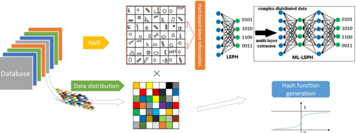
Fig. 1 The outline of the proposed method. Part-based latent informa-tion is learned from NMF with the regularizainforma-tion of data distribuinforma-tion. We propose two different versions of our algorithm, i.e., single layer

LSPH and multi-layer LSPH. Specifically, ML-LSPH generates deep data representations which can theoretically lead to better performance for retrieval tasks with more complex data

to maintain the similarity between high-dimensional data and low-dimensional codes. Moreover, incorporated with the representation of binary codes, the part-based latent infor-mation obtained by NMF based hashing, i.e., LSPH, could be regarded as independent latent attributes of samples. In other words, the binary codes determine whether the high-dimensional data hits the corresponding latent attributes or not. Given an image, this kind of data-driven attributes can allow us to well describe an image and also may benefit zero-shot learning (Jayaraman and Grauman 2014;Lampert et al. 2014;Tao 2015;Yu et al. 2013) for unseen image classifica-tion/retrieval in future work.

Specifically, because of the limitation of NMF, which cannot completely discover the latent structure of the orig-inal high-dimensional data, we provide a new objective function to preserve as much of the probabilistic distribu-tion structure of the high-dimensional data as possible to the low-dimensional map. Meanwhile, we propose an opti-mization framework for the objective function and show the updating rules. Besides, to implement the optimiza-tion process, the training data are relaxed into a real-valued range. Then, we convert the real-valued representations into binary codes. Finally, we analyze the experimental results and compare them with several existing hashing algorithms. The outline of the proposed LSPH approach is depicted in Fig.1.

LSPH is a linear hashing technique with a single-layer generative network and data distribution preserving con-straints. Although it is an efficient binary coding method for large-scale retrieval tasks, such a single-layer generative net-work may lead to several limitations in the following cases as mentioned in [1]: (1) when it learns data which lie on or near a nonlinear manifold; (2) when it learns syntactic

rela-tionships of given data; and (3) when it learns hierarchically generated data. The single-layer LSPH is apparently not fit for such cases. For instance, LSPH with a single-layer net-work can well tackle data with small intra-variations such as face images. However, for more complex data with extremely different viewpoints, additional degrees of freedom of the data will be required. In terms of large-scale image retrieval tasks, the sources of data can be very variant and even sam-ples belonging to the same category can differ significantly. Naturally, the single-layer LSPH is not competent for simi-larity search on such heterogeneous databases.

Therefore, in this paper, we also propose an extension of LSPH called multi-layer LSPH (ML-LSPH) with the multi-layer generative network [1] and distribution preserv-ing constraints. ML-LSPH can deeply learn part-based latent information of data and preserve the joint probabilistic distri-bution for deep data representations. Applying the sigmoid function to each layer, ML-LSPH is a nonlinear architecture. Similar to recent deep neural networks (Hinton et al. 2006;

Masci et al. 2011;Krizhevsky et al. 2012), ML-LSPH gen-erates deep data representations which can theoretically lead to better performance than single layer LSPH for retrieval tasks with more complex data2_{in realistic scenarios.} How-ever, ML-LSPH is computationally more expensive during training and test phases compared to single layer LSPH. Thus, there exists a trade-off between ML-LSPH and LSPH in terms of performance and computational complexity, and the choice between these two versions depends on the requirement of the application. Besides, as ML-LSPH is a generalized framework of LSPH, it can easily shrink to LSPH

2 _{Such data have large intra-class variations but small inter-class} vari-ations, e.g., large-scale retrieval on fine-grained data.

if the number of the layers is set to1. We evaluate our LSPH and ML-LSPH on three large-scale datasets: SIFT 1M, GIST 1M and TinyImage, and the results show that our methods significantly outperform the state-of-the-art hashing tech-niques. It is worthwhile to highlight several contributions of the proposed methods:

– LSPH can learn compact binary codes uncovering the latent semantics and simultaneously preserving the joint probability distribution of data.

– We utilize multivariable logistic regression to gener-ate the hashing function and achieve the out-of-sample extension.

– To tackle the data with more complex distribution, a multi-layer extension of LSPH (i.e., ML-LSPH) has been proposed for large-scale retrieval as well.

The rest of this paper is organized as follows. In Sect.2, we give a brief review of NMF. The details of LSPH and ML-LSPH are described in Sects.3and4, respectively. Section5

reports the experimental results. Finally, we conclude this paper and discuss the future work in Sect.6.

2 A Brief Review of NMF

In this section, we mainly review some related algorithms, focusing on Nonnegative Matrix Factorization (NMF) and its variants. NMF is proposed to learn the nonnegative

parts of objects. Given a nonnegative data matrix X =

[x1,· · ·,xN] ∈RM_≥0×N, each column ofX is a sample data.

NMF aims to find two nonnegative matricesU∈R_≥M₀×Dand

V ∈R_≥D₀×Nwith full rank whose product can approximately represent the original matrix X, i.e.,X ≈U V. In practice, we always set D < min(M,N). The target of NMF is to minimize the following objective function

LN M F= X−U V2, s.t.U,V ≥0, (1)

where · is the Frobenius norm. To optimize the above

objective function, an iterative updating procedure was devel-oped inLee and Seung(1999) as follows:

Vi j ← UTX_{i j} UT_{U V} i j Vi j, Ui j ← X VT_{i j} U V VT i j Ui j, (2) and normalization Ui j ← Ui j iUi j. (3) It has been proved that the above updating procedure can find the local minimum ofLN M F. The matrixV obtained in

NMF is always regarded as the low-dimensional representa-tion while the matrixUdenotes the basis matrix.

Furthermore, there also exists some variants of NMF. Local NMF (LNMF) (Li et al. 2001) imposes a spatial local-ized constraint on the bases. InHoyer(2004), sparse NMF was proposed and later, NMF constrained with neighborhood preserving regularization (NPNMF) (Gu and Zhou 2009) was developed. Besides, researchers also proposed graph

regu-larized NMF (GNMF) (Cai et al. 2011), which effectively

preserves the locality structure of data. Beyond these meth-ods,Zhang et al.(2006) extends the original NMF with the kernel trick as kernelized NMF (KNMF), which could extract more useful features hidden in the original data through some kernel-induced nonlinear mappings. Additionally, a hashing method based on multiple kernels NMF was proposed in

Liu et al. (2015), where an alternate optimization scheme is applied to determine the combination of different ker-nels.

In this paper, we present a Latent Structure Preserving NMF framework for hashing (i.e., LSPH), which can effec-tively preserve the data intrinsic probability distribution and simultaneously reduce the redundancy of low-dimensional representations. Specifically, since the solution of standard NMF only focuses on optimizing matrix factorization to min-imize Eq. (1), the obtained low-dimensional representation

V lacks the data relationship information. In fact, most of previous NMF extensions are based on keeping the local-ity regularization to guarantee that, if the high-dimensional data points are close, the low-dimensional representations from NMF can still be close. However, this kind of reg-ularization may lead to a low-quality factorization, since it ignores preserving the whole data distribution but only focuses on locality information. For a realistic scenario with noisy data, locality preserving regularization would even pro-duce worse performance. Rather than locality-based graph regularization, we measure the joint probability of data by Kullback-Leibler divergence, which is defined over all of the potential neighbors and has been proved to effectively resist data noise (Maaten and Hinton 2008). This kind of measurement reveals the global structure such as the pres-ence of clusters at several scales. To make LSPH more capable on data with more complex distributions, the multi-layer LSPH (ML-LSPH) is also proposed, in which more discriminative, high-level representations can be learned from a multi-layer network with the distribution preserv-ing regularization term. To the best of our knowledge, this is the first time that multi-layer NMF based hashing is successfully applied to feature embedding for large-scale similarity search. A preliminary version of our LSPH has been presented inCai et al.(2015). In this paper, we include more details and experimental results and extend LSPH to ML-LSPH for more complex data in realistic retrieval appli-cations.

3 Latent Structure Preserving Hashing

In this section, we mainly elaborate the proposed Latent Structure Preserving Hashing algorithm.

3.1 Preserving Data Structure with NMF

NMF is an unsupervised learning algorithm which can learn a parts-based representation. Theoretically, it is expected

that the low-dimensional dataV given by NMF can obtain

locality structure from the high-dimensional data X. How-ever, in real-world applications, NMF cannot discover the intrinsic geometrical and discriminating structure of the data space. Therefore, to preserve as much of the significant structure of the high-dimensional data as possible, we pro-pose to minimize the Kullback-Leibler divergence (Xie et al. 2011) between the joint probability distribution in the high-dimensional space and the joint probability distribution that is heavy-tailed in the low-dimensional space:

C=λK L(PQ). (4)

In Eq. (4), P is the joint probability distribution in the high-dimensional space which can also be denoted as pi j. Q is the joint probability distribution in the low-dimensional space that can be represented asqi j.λis the control of the smoothness of the new representation. The conditional prob-ability pi j means the similarity between data pointsxi and xj, wherexjis picked in proportion to their probability den-sity under a Gaussian centered atxi. Since only significant points are needed to model pairwise similarities, we setpii andqii to zero. Meanwhile, it has the characteristics that

pi j = pj i andqi j =qj i for∀i,j. The pairwise similarities in the high-dimensional spacepi j are defined as:

pi j = exp−xi−xj2/2σi2 k=lexp −xk−xl2/2σk2 , (5)

whereσiis the variance of the Gaussian distribution which is centered on data pointxi. Each data pointximakes a signifi-cant contribution to the cost function. In the low-dimensional map, using the probability distribution that is heavy tailed, the joint probabilitiesqi jcan be defined as:

qi j = 1+ vi−vj2 ₋1 k=l 1+ vk−vl2 ₋1. (6)

This definition is an infinite mixture of Gaussians, which is much faster to evaluate the density of a point than the sin-gle Gaussian, since it does not have an exponential. This representation also makes the mapped points invariant to the changes in the scale for the embedded points that are far apart.

Thus, the cost function based on Kullback-Leibler divergence can effectively measure the significance of the data distribu-tion .qi j modelspi j is given by

G=K L(PQ)=

i

j

pi jlogpi j −pi jlogqi j. ₍₇₎

For simplicity, we define two auxiliary variablesdi j and Z for making the derivation clearer as follows:

di j = vi −vjandZ = k=l 1+d_kl2 ₋1 . (8)

Therefore, the gradient of functionGwith respect tovi can be given by ∂G ∂vi = 2 N j₌1 ∂G ∂di j vi−vj . (9)

Then_∂∂_{di j}G can be calculated by Kullback-Leibler divergence in Eq. (7): ∂G ∂di j = − k=l pkl ⎛ ⎝ 1 qklZ ∂1+d_kl2−1 ∂di j − 1 Z ∂Z ∂di j ⎞ ⎠_. (10) Since ∂((1+d 2 kl)−1)

∂di j is nonzero if and only ifk=iandl= j, andk₌l pkl=1, the gradient function can be expressed as

∂G

∂di j

=2pi j −qi j 1+di j2

₋1

. (11)

Eq. (11) can be substituted into Eq. (9). Therefore, the gra-dient of the Kullback-Leibler divergence between P and Q is ∂G ∂vi = 4 N j₌1 (pi j−qi j)(vi −vj) 1+ vi−vj2 ₋1 . (12) Therefore, through combining the data structure preserv-ing part in Eq. (4) and the NMF technique, we can obtain the following new objective function:

Of = X−U V2+λK L(PQ), (13)

where V ∈ {0,1}D×N, X,U,V 0, U ∈ RM×D, X ∈

RM×N_{, andλcontrols the smoothness of the new} represen-tation.

In most of the circumstances, the low-dimensional data only from NMF is not effective and meaningful for realistic applications. Thus, we introduceλK L(PQ)to preserve the structure of the original data which can obtain better results in information retrieval.

3.2 Relaxation and Optimization

Since the discreteness conditionV ∈ {0,1}D×N in Eq. (22) cannot be calculated directly in the optimization procedure, motivated byWeiss et al.(2009), we first relax the dataV ∈ {0,1}D×Nto the rangeV ∈RD×Nfor obtaining real-values. Then let the Lagrangian of our problem be:

L= X−U V2+λK L(PQ)+tr

ΦUT

+tr(ΨVT), (14)

where matricesΦandΨare two Lagrangian multiplier matri-ces. Since we have the gradient ofC =λG:

∂C ∂vi = 4λ N j=1 pi j −qi j vi−vj 1+ vi−vj2 ₋1 , (15) we make the gradients ofLbe zeros to minimizeOf:

∂L ∂V =2 −UTX+UTU V +∂_∂vC i +Ψ =0, (16) ∂L ∂U =2 −X VT +U V VT +Φ =0, (17)

In addition, we also have KKT conditions:Φi jUi j =0 and Ψi jVi j =0,∀i,j. Then multiplyingVi j andUi j in the cor-responding positions on both sides of Eqs. (16) and (17) respectively, we obtain 2 −UTX+UTU V + ∂C ∂vi i j Vi j =0, (18) 2 −X VT +U V VT i jUi j =0. (19) Note that _∂ C ∂vj i = 4λ N k=1 pj kvj −qj kvj−pj kvk+qj kvk 1+ vj −vk2 i =4λ N k₌1 pj kVi j−qj kVi j−pj kVi k+qj kVi k 1+ vj−vk2 .

Therefore, we have the following update rules for anyi,j:

Vi j ← UTX_{i j}+2λ N k=1 pj kVi k+qj kVi j 1+vj−vk2 UT_{U V} i j +2λ N k₌1 pj kVi j+qj kVi k 1+vj−vk2 Vi j, (20) Ui j ← X VT_{i j} U V VT i j Ui j. (21)

All the elements inUandVcan be guaranteed that they are nonnegative from the allocation. InLee and Seung(2000), it has been proved that the objective function is monotonically

non-increasing after each update ofU or V. The proof of

convergence aboutUandV is similar to the ones inZheng

et al.(2011),Cai et al.(2011).

Once the above algorithm is converged, we can obtain the real-valued low-dimensional representation by a linear pro-jection matrix. Since our algorithm is based on general NMF

rather than Projective NMF (PNMF) (Yuan and Oja 2005;

Guan et al. 2013), a direct projection does not exist for data embedding. Thus, in this paper, inspired byCai et al.(2007), we consider using linear regression to compute our projec-tion matrix. Particularly, we make the projecprojec-tion orthogonal

by solving the Orthogonal Procrustes problem (Schönemann

1966) as follows: min

P PX−V, s.t.P T_{P =}

I (22)

whereP is the orthogonal projection. The optimal solution can be obtained by the following procedure: 1. use the singu-lar value decomposition algorithm to decompose the matrix

XTV = AΣBT; 2. calculateP = BΩAT, where,Ω is a connection matrix asΩ = [I,0] ∈RD×M _{and0indicates} all zeros matrix. Given datax∈RM×1, its low-dimensional

representation is v = Px. There are three advantages on

using orthogonal projection according toZhang et al.(2015): Firstly, the orthogonal projection can preserve the Euclid-ean distance between two points; Secondly, the orthogonal projection can distribute the variance more evenly across the dimensions; Thirdly, the orthogonal projection can learn maximally uncorrelated dimensions, which leads to more compact representations.

3.3 Hash Function Generation

The low-dimensional representations V ∈ RD×N and the

basesU ∈ RM×D, where D M, can be obtained from

Eq. (20) and Eq. (21), respectively. Then we need to convert

the low-dimensional real-valued representations from V =

[v1,· · ·,vN]into binary codes via thresholding: if thed-th

value will be represented as 1; otherwise it will be 0, where

d=1,· · ·,Dandn =1,· · · ,N.

In addition, a well-designed semantic hashing should also be entropy maximizing to ensure its efficiency (Baluja and Covell 2008). Meanwhile, from the information theory, through having a uniform probability distribution, the source alphabet can reach a maximal entropy. Specifically, if the entropy of codes over the corpus is small, the documents will be mapped to a small number of codes (hash bins). In this paper, the threshold of the elements invncan be set to the median value ofvn, which can satisfy entropy maximization. Therefore, half of the bit-strings will be 1 and the other half will be 0. In this way, the real-value code can be calculated into a binary code (Yu et al. 2014).

However, from the above procedure, we can only obtain the binary codes of the data in the training set. Therefore, given a new sample, it cannot directly find a hash function. To solve such an “out-of-sample” problem, in our approach, we are inspired by the “self-taught” binary coding scheme (Zhang et al. 2010) to use the logistic regression ( Hos-mer and Lemeshow 2004) which can be treated as a type of probabilistic statistical classification model to compute the hash code for unseen test data. Specifically, we learn a square projection matrix via logistic regression, which can be regarded as a rotation ofV. This kind of transformation

can make the codes more balanced (Gong et al. 2013;Liu

et al. 2012) and lead to better performance compared with directly binarizingV with the median value calculated from training data. To make it more convincing, we also show the performance difference in the later section. Before obtain-ing the logistic regression cost function, we define that the binary code is represented as Vˆ = [ˆv1,· · · ,vˆN], where

ˆ

vn ∈ {0,1}D and n = 1,· · ·,N. Therefore, the training

set can be considered as{(v1,vˆ1), (v2,vˆ2),· · · , (vN,vˆN)}. The vector-valued regression function which is based on the

corresponding regression matrixΘ ∈ RD×D _{can be}

repre-sented as h_Θ(vn)= 1 1+e−(ΘTvn)_i T i=1,···,D . (23)

Therefore, with the maximum log-likelihood criterion for the Bernoulli-distributed data, our cost function for the cor-responding regression matrix can be defined as:

J(Θ)= − 1 N N n=1 ˆ vT_nlog(h_Θ(vn)) +(1− ˆvn)Tlog(1−hΘ(vn)) +δΘ2_, (24)

wherelog(·)is the element-wise logarithm function and1is anD×1 all ones matrix. We useδΘ2as the regularization term in logistic regression to avoid overfitting.

To find the matrixΘwhich aims to minimizeJ(Θ), we

use gradient descent and repeatedly update each parameter using a learning rateα. The updating equation is shown as follows: Θ(t+1)_=Θ(t)₋ α N N i=1 h_Θ(t)(vi)− ˆvi vT_i −αδ N Θ (t)_. (25) The updating equation stops when the norm of difference betweenΘ(t+1)_andΘ(t)_{, i.e.,||Θ}(t+1)_−Θ(t)_||2_{, is smaller} than a small value. Then we can obtain the regression matrix Θ. For a new coming test dataXnew ∈RM×1, then its low-dimensional representation isVnew =PXnew. Note that each entry ofh_Θis a sigmoid function, the hash codes for a new coming sampleXnew∈RM×1can be represented as:

ˆ

Vnew= hΘ(PXnew), (26)

where·means the nearest integer function for each entry

of h_Θ. Specifically, since the output of logistic regression i.e., h_Θ(PXnew), indicates the probability of “1” for each entry, · is equivalent to binarizing each bit by probabil-ity 0.5. Thus, if the probability of a bit from h_Θ(PXnew) is larger than 0.5, it will be represented as 1, otherwise 0. For example, through Eq. (26), vector h_Θ(PXne_w) =

[0.17,0.37,0.42,0.79,0.03,0.92,· · · ]can be expressed as

[0,0,0,1,0,1,· · · ]. Up to now, we can obtain the Latent

Structure Preserving Hashing codes for both training and test data. The procedure of LSPH is summarized in Algorithm 1.

Algorithm 1Latent Structure Preserving Hashing (LSPH) Input:

The training matrix X ∈ _RM×N_{; the objective dimension (code}

length)Dof hash codes; the learning rateαfor logistic regression; the regularization parameters {δ,λ}.

Output:

The basis matrixU, the orthogonal projectionPand the regression matrixΘ.

1: Initialize U and V with uniformly distributed random values between 0 and 1.

2:repeat

3: Compute the low-dimensional representation matrixV and the basis matrixUvia Eqs. (20) and (21), respectively;

4:untilconvergence

5: SVD decompose the matrixXT_{V to obtain AΣB}T _{and calculate}

P=BΩAT_;

6: Obtain the regression matrixΘthrough Eq. (25) and the final LSPH encoding for each sample is defined in Eq. (26).

4 Multi-Layer LSPH Extension

To better tackle the retrieval tasks with more complex data distributions, in this section, we introduce the multi-layer

……

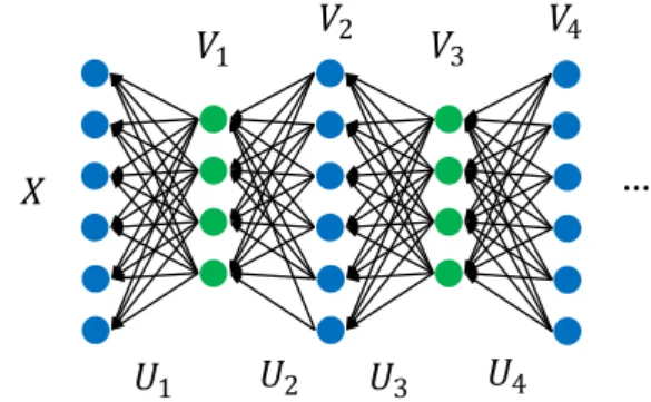
Fig. 2 Illustration of multi-layer LSPH (ML-LSPH)

LSPH (ML-LSPH). ML-LSPH aims to generate more infor-mative high-level representations compared with single-layer LSPH for data with complex distributions. Once the represen-tation by ML-LSPH is computed, the final hashing functions are also obtained through multivariable logistic regression, same as LSPH mentioned above.

Given data matrixX ∈ RM×N, inspired by recent deep

learning algorithms and multi-layer NMF [1], Trigeorgis

et al.(2014), we can extract latent data attributes by incor-porating our LSPH algorithm with a multi-layer structure as illustrated in Fig.2. Similar to the learning of the above rep-resentation matrixV, a matrix sequenceV1,· · ·,Vncan be obtained by solving the following optimization problems:

minX−U1V12+λK L P||Q(1) minV1−U2V22+λK L P||Q(2) ... minVn−1−UnVn2+λK L P||Q(n) , whereUi ∈ RDi−1×Di,Vi ∈ RDi×N,i =1,· · · ,n, D0 =

M,P is the distribution ofXandQ(i)is the distribution of

Vi. ∂Gj ∂Ui = U_iT₋₁· · ·U_jT₊₁ ∂K LP||Q(j) ∂Vj gUj+1Vj+1 · · · g(UiVi) V_iT (27) ∂Gj ∂Vi = U_iTU_iT₋₁· · ·UT_j+1 ∂K LP||Q(j) ∂Vj gUj+1Vj+1 · · · g(UiVi) (28) (Ui)μν←(Ui)μν ⎛ ⎜ ⎝ RiViT μν+λ i j=1 M_i(₋j)₁g(UiVi) V_iT μν NiViT μν+λij=1 S_i(₋j)₁g(UiVi) V_iT μν ⎞ ⎟ ⎠ γ (29) (Vi)μν←(Vi)μν ⎛ ⎜ ⎝ UT i Ri_μν+λij=1UiT M_i(₋j)₁g(UiVi) μν UT i Ni μν+λ i j=1UiT S_i(₋j)₁g(UiVi) μν ⎞ ⎟ ⎠ γ (30)

In this way,Vi,i = 1,· · · ,n, are the hidden factors of each layer. By introducing the nonlinear functiong(·)into the network, these hidden factors are generated by the following rules:

Vi =g(Ui+1Vi+1) , i =n−1,· · · ,0. (31)

Then our task is to minimize the following objective function:

F = X−g(U1g(U2· · ·g(UnVn)))2 +λ n i=1 K L P||Q(i) . (32)

Let us denoteGi = K L(P||Q(i))andis the Hadamard product (element-wise product). By taking the derivatives of

F with respect toUi andVi, we have: ∂F ∂Ui =( Ni−Ri)ViT +λ i j₌1 ∂Gj ∂Ui (33) ∂F ∂Vi = U_iT(Ni−Ri)+λ i j=1 ∂Gj ∂Vi (34)

where matricesNi,Ri ∈RDi−1×N are calculated by the fol-lowing rules: Ri+1= UiTRi g(Ui+1Vi+1) Ni₊1= UiTNi g(Ui₊1Vi₊1)

fori =1,· · ·,n−1, with the initialization:

R1= Xg(U1V1)

N1=(U1V1)g(U1V1) .

Besides, the derivatives ofG with respect toUi andVi are calculated by Eqs. (27) and (28). With the derivation in Sect.3, we have the derivative

∂K L(P||Q(j)₎ ∂Vj μν =4 N k₌1 p_νk(Vj)μν−q_ν(_kj)(Vj)μν−pνk(Vj)μk+q_ν(_kj)(Vj)μk 1+vνj−v_kj2 ,

where v_kj is the k-th column of Vj,k = 1,· · ·,N and

j = 1,· · ·,n. To ensure that every element inUi andVi

is nonnegative, we use the following symbols to split the above derivatives as:

∂K LP||Q(j) ∂Vj = Aj−Bj, (35) where Aj μν =4 N k=1 p_νk(Vj)_μν+q_ν(_kj)(Vj)_μk 1+ v_νj−v_kj2 , (36) Bj μν =4 N k=1 q_ν(_kj)(Vj)μν+pνk(Vj)μk 1+ v_νj−v_kj2 . (37)

Then we can define two matrix sequencesSl andMl as fol-lows: S_l(₊j)₁=U_lT₊₁ S_l(j)g(Ul+1Vl+1) , (38) M_l(₊j)₁=U_lT₊₁ M_l(j)g(Ul+1Vl+1) , (39)

wherel = j,· · ·,i −2,S(_jj) = Aj andM(_jj) =Bj. In this way, the derivatives ofGjwith respect toUiandVi, i.e., Eqs. (27) and (28), will be:

∂Gj ∂Ui = (S_i(₋j)₁−M_i(₋j)₁)g(UiVi) V_iT, (40) ∂Gj ∂Vi = U_iT (S_i(₋j)₁−M_i(₋j)₁)g(UiVi) . (41)

Substitute the above equations into Eqs. (33) and (34), we obtain: ∂F ∂Ui =( Ni−Ri)ViT +λ i j=1 (S_i(₋j)₁−M_i(₋j)₁)g(UiVi) V_iT, ∂F ∂Vi = U_iT(Ni−Ri) +λ i j=1 U_iT (S_i(₋j)₁−M_i(₋j)₁)g(UiVi) .

Finally, similar to the procedure in Sect. 3, the update rules for multi-layer LSPH (ML-LSPH) are shown in Eqs. (29) and (30), where 0 < γ < 1 is the learning rate

andi = 1,· · ·,n. The convergence property of the above

iteration is similar to the one in [1]. Besides, for better under-standing our ML-LSPH, we aim to unify the LSPH and ML-LSPH under a same framework. Thus, in our implemen-tation, the function g(·)applied onU1 andV1 is regarded

as identity function f(x) = x. The function g(·)for Ui

andVi,i =2,· · · ,n is played by nonlinear sigmoid

func-tion f(x)= ₁₊1_ex. In this way, when the number of layers

n = 1, the ML-LSPH will shrink to the ordinary

single-layer LSPH. It is noteworthy that we could theoretically formulate our ML-LSPH to an arbitrary number of lay-ers according the above algorithms. However, for realistic applications with complex data distributions, the number of layers is always less than 3, since when the number of layers increases, the accumulative reconstruction error will cause the non-convergence of the proposed model (Trigeorgis et al. 2014).

For the hash code generating phase, it is similar to LSPH. In particular, acquired the low-dimensional representation

Vnin then-th layer, we first solve the Orthogonal Procrustes problem min_PT_P=IPX −Vnto achieve the orthogonal projectionP. The optimal solution can be obtained by the following procedure: 1. use the singular value decomposi-tion algorithm to decompose the matrixXTVn =AΣBT; 2. calculateP = BΩAT, where,Ωis a connection matrix as Ω = [I,0] ∈RD×M and0indicates all zeros matrix. For a new coming test dataxnew ∈ RM×1, the low-dimensional representation in the n-th layer is vnen w = Pxne_w and the binary codes are calculated by vˆne_n w = h_Θ(Pxnew)

where Θ is obtained by the similar multi-variable

regres-sion scheme. The procedure of ML-LSPH is summarized in Algorithm2.

Algorithm 2Multi-layer Latent Structure Preserving Hash-ing (ML-LSPH)

Input:

The training matrix X ∈ RM×N; the dimensions for n layers

D₁,· · ·,D_n; the learning rateγ for the multi-layer NMF struc-ture; the learning rateαfor logistic regression; the regularization parameters {δ,λ}.

Output:

Then-th layer representationVn, the orthogonal projectionPand

the regression matrixΘ.

1: Initialize Ui and Vi with uniformly distributed random values

between 0 and 1,i=1,· · ·,n. 2:repeat

3: Compute the basis matrixUiand the low-dimensional

represen-tation matrixVivia Eqs. (29) and (30) respectively for each layer;

4:untilconvergence

5: SVD decomposes the matrixXTVnto obtainAΣBT and calculate

P=BΩAT;

6: Obtain the regression matrixΘthrough Eq. (25) and the final ML-LSPH encoding for each sample is defined byh_Θ(PX).

Batch-Based Learning SchemeWith the number of the layers

increasing, the computational costs will inevitably increase as well in the current multi-layer network architecture of ML-LSPH. In order to effectively reduce the computa-tional complexity on large-scale data, we adopt a random batch-based learning strategy (RBLS) in the iteration

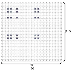
opti-Fig. 3 Illustration of the P ∈ RN×N and Q(j) ∈ RN×N matrices composition. Thewhite blocksindicate zeros anddark-colored blocks

indicate the similarity computed via the randomly selected subset

mization of ML-LSPH. The complexity of each layer’s NMF

isO(N M D)as mentioned above, which is still regarded as

linear complexity in terms ofNand not very demanding for large-scale data processing. However, the real bottleneck of the optimization procedure is the calculation of the KL diver-gence for each layer, specifically, the similarity matricesP

andQ(m), due to the complexity ofO(N2D). Therefore, in our implementation, we adopt RBLS to effectively reduce

the complexity for computing P and Q(m) in ML-LSPH.

In detail, for each step of updating P and Q(m), we ran-domly select a small subset of the whole training set. Then we only need to compute the pairwise similarity of this subset and the rest of the elements ofPandQ(m)are replaced by zeros: pi j = ⎧ ⎨ ⎩ exp(−xi−xj2/2σi2) k=lexp(−xk−xl2/2σk2), ifxi,xj ∈batch 0, otherwise , q_{i j}m = ⎧ ⎨ ⎩ (1+vm_i −vm_j2)−1 k=l(1+vmk−vml 2)−1, ifv m i ,v m j ∈batch 0, otherwise ,

where m indicates the layer index. The illustration of pro-posed RBLS are also shown in Fig.3. If we assume the size of the small subset is, the complexity of our RBLS will be reduced fromO(N2D)toO(2D). Usually, thecan be set as=1/100N. It is noteworthy that only the computation of

PandQ(m)are replaced by the above RBLS trick and other parts of the algorithm in ML-LSPH are still the same as men-tioned before. In this way, our multi-layer LSPH becomes scalable for large-scale data.

5 Computational Complexity Analysis

In this section, we will discuss the computational complexity of LSPH and ML-LSPH. The computational complexity of LSPH consists of three parts. The first part is for comput-ing NMF, the complexity of which is O(N M D)(Li et al.

2014), where N is the size of the dataset, M and D are

the dimensionalities of the high-dimensional data and the low-dimensional data respectively. The second part is to compute the cost function Eq. (7) in the objective func-tion which has the complexityO(N2D). The last part is the logistic regression procedure whose complexity isO(N D2). Therefore, the total computational complexity of LSPH is:

O(t N M D+N2D+t N D2), wheretis the number of

iter-ations.

It is obvious that single-layer ML-LSPH is actually LSPH. The computational complexity of ML-LSPH with multiple layers consists of several NMF optimizations, the computation of matrices P and Q(j), and the logistic regression procedure. With the above discussion, the com-putational complexity of ML-LSPH isO(t N Mn_i=1Di+ 2n

i=1Di+t N D2), whereis the batch size.

6 Experiments and Results

In this section, we systematically evaluate the proposed LSPH and multi-layer LSPH (ML-LSPH) on three large-scale datasets. The relevant experimental results and data visualization will be included in the rest of this section. All the experiments are completed using MatLab2014a on a

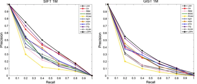
work-Fig. 5 The precision-recall curves of the compared algorithms on the SIFT 1M and GIST 1M datasets for the code of 48 bits (Color figure online)

Table 1 The comparison of MAP between using median values and Logistic regression to generate codes with different numbers of bits

Code length 16 bits 32 bits 48 bits 64 bits 80 bits 96 bits SIFT 1M

Median value binarization 0.274 0.321 0.355 0.390 0.427 0.448 Logistic regression binarization 0.303 0.340 0.376 0.424 0.445 0.461

GIST 1M

Median value binarization 0.131 0.157 0.193 0.207 0.214 0.227 Logistic regression binarization 0.153 0.185 0.211 0.234 0.241 0.255

Table 2 The comparison of MAP, training time and test time of 32 bits and 48 bits of all the compared algorithms on the SIFT 1M dataset

Methods SIFT 1M

32 bits 48 bits

MAP Train time (s) Test time (µs) MAP Train time (s) Test time (µs)

LSH 0.240 0.3 1.1 0.280 0.6 1.9 KLSH 0.150 10.5 14.6 0.230 10.7 16.2 RBM 0.260 4.5×104 _{3.3 0.280 5.8×10}4 _3.7 BSSC 0.280 2.2×103 11.2 0.293 2.6×103 13.4 PCAH 0.252 6.5 1.2 0.235 7.4 1.9 SpH 0.275 25.8 28.3 0.284 88.2 101.9 AGH 0.161 144.7 55.7 0.267 184.2 72.0 ITQ 0.320 1.0×103 _{32.1 0.360 1.1×10}3 _35.7 STH 0.270 1.2×103 _{17.4 0.318 1.8×10}3 _19.8 CH 0.280 93.4 53.5 0.330 98.2 54.4 LSPH 0.340 1.1×103 20.3 0.376 1.2×103 22.7

Table 3 The comparison of MAP, training time and test time of 32 bits and 48 bits of all the compared algorithms on the GIST 1M dataset

Methods GIST 1M

32 bits 48 bits

MAP Train time (s) Test time (µs) MAP Train time (s) Test time (µs)

LSH 0.107 1.4 2.7 0.135 2.1 3.0 KLSH 0.110 29.5 27.2 0.120 30.7 38.0 RBM 0.123 5.5×104 _{3.4 0.142 6.2×10}4 _3.7 BSSC 0.112 3.2×103 _{13.0 0.130 3.8×10}3 _15.1 PCAH 0.090 49.2 2.8 0.075 52.3 3.0 SpH 0.130 65.3 40.2 0.148 131.1 116.3 AGH 0.124 242.5 83.7 0.160 279.4 95.6 ITQ 0.170 1.2×103 _{33.8 0.200 1.5×10}3 _36.2 STH 0.123 1.9×103 _{21.3 0.171 2.5×10}3 _25.2μ CH 0.160 194 64.1 0.190 210.5 71.5 LSPH 0.185 1.4×103 21.8 0.211 1.7×103 24.1

Fig. 6 Some example images from the TinyImage dataset (Color figure online)

station with a 12-core 3.2GHz CPU and 120GB of RAM running the Linux OS.

6.1 Evaluation on LSPH

In this subsection, we first apply the proposed single-layer LSPH algorithm method for large-scale similarity search tasks. Two realistic datasets are used to evaluate all meth-ods:SIFT 1M: it contains one million 128-dim local SIFT feature vectors (Lowe 2004).GIST 1M: it contains one mil-lion 960-dim global GIST feature vectors (Oliva and Torralba 2001). The two datasets are publicly available.3

3_{http://corpus-texmex.irisa.fr.}

For both SIFT 1M and GIST 1M, we respectively take

10K images as the queries by random selection and use

the remaining to form the gallery database. To construct the training set, 200,000 samples from the gallery database are randomly selected for all of the compared methods. Addition-ally, we also randomly choose another 50,000 data samples as a cross-validation set for parameter tuning. In the querying phase, the returned points are regarded as true neighbors if they lie in the top 2 percentile points closest to a query for both two datasets. Since the Hamming lookup table is fast with hash codes, we will use the Hamming lookup table to measure our retrieval tasks. We evaluate the retrieval results in terms

Fig. 7 The top-500 Mean Average Precision of the compared algo-rithms on the TinyImage dataset (Color figure online)

of the Mean Average Precision4(MAP) and the

precision-recall curves. Additionally, we also report the training time and the test time (the average searching time used for each query) for all methods.

6.1.1 The Selected Methods and Settings

In this experiment, we compare LSPH with the 10 selected popular hashing methods including LSH (Gionis et al. 1999),

BSSC (Shakhnarovich 2005), RBM (Salakhutdinov and

Hin-ton (2007)), SpH (Weiss et al. 2009), STH (Zhang et al. 2010), AGH (Liu et al. 2011), ITQ (Gong et al. 2013), KLSH (Kulis and Grauman 2009), PCAH (Wang et al. 2012) and CH (Lin et al. 2013). In these methods, for BSSC, through the labeled pairs scheme in the boosting framework, it can obtain weights and thresholds for every hash function. RBM will be trained with several 100-100 hidden layers without fine-tuning. According to KLSH, 500 training samples and the RBF-kernel are used to output the empirical kernel map, in which we always set the scalar parameterσ to an appro-priate value on each dataset. For ITQ, the number of the iterations is set as 50. In AGH with two-layer, we consider the number of the anchor pointskas 200 and the number of the nearest anchorssin sparse coding as 50. CH has the same anchor-based sparse coding setting with AGH. All of the 10 methods are evaluated on different lengths of the codes, e.g., 16, 32, 48, 64, 80 and 96. Under the same experimental set-ting, all the parameters used in the compared methods have been strictly chosen according to their original papers.

4_{The ground-truth is defined by top 2 percentile nearest neighbors of} a query via linear scan based on the Euclidean distance.

In the experiments of our LSPH method, all the data are first normalized into the range of[0,1], since the nonnegative constraint is required in our framework. We also use the vali-dation set to tune our hyper-parameters. Particularly, for each dataset, we select one value from{0.01,0.02,· · ·,0.10}as the optimal learning rateαof multi-variable logistic regres-sion through 10-fold cross-validation on the validation set.

The regularization parameter λ is determined from one of

{10−2,10−1,1,101,102,103}, which yields the best perfor-mance via 10-fold cross-validation on the validation set. The regularization parameterδin the hash function generation is fixed asδ =0.35. We limit the maximum number of itera-tions with 1000 in LSPH learning phase, as well.

6.1.2 Results Comparison

We demonstrate MAP curves on the SIFT 1M and GIST 1M datasets compared with different methods in Fig.4. From the general tendency, the accuracies on the GIST 1M dataset are lower than those on the SIFT 1M dataset, since features in the GIST 1M has higher dimensions with larger variations than those on SIFT 1M. In detail of Fig.4, ITQ always achieves higher Mean Average Precision (MAP) and gets a consis-tent increasing condition with the change of the code length on both datasets. Furthermore, MAP of CH also proves to be competitive but a little lower than ITQ. Interestingly, on both the SIFT 1M and GIST 1M datasets, the MAP of SpH and STH are always “rise-then-fall” when the length of code increases. Due to the use of random projection, LSH and KLSH have a low MAP when the code length is short. More-over, PCAH always gets decreasing accuracies when the code length increases. For our method LSPH, it achieves the high-est performance among all the compared methods on both datasets. The proposed LSPH algorithm can automatically exploit the latent structure of the original data and simul-taneously preserve the consistency of distribution between the original data and the reduced representations. The above properties of LSPH allow it to achieve better performance in large-scale visual retrieval tasks. Fig. 5 also shows the precision-recall curves with the code length of 48 bits on both SIFT 1M and GIST 1M datasets with the top 2 per-centile nearest neighbors as the ground truth. From all these figures, we can further discover that, for both two datasets, LSPH achieves apparently better performance than other hashing methods by comparing the Mean Average Precision (MAP) and Area Under the Curve (AUC). Additionally, to further illustrate the necessity of using logistic regression binarization rather than direct median value binarization as mentioned in Sect.3.3, we carry out comparison experiments on both SIFT 1M and GIST 1M datasets. In Table1, it is easy to observe that logistic regression binarization can achieve consistently higher MAP across all code lengthes than the direct median value binarization scheme.

Fig. 8 Comparison of precision recall curves with different bits on the TinyImage dataset. Ground truth is defined by top-500 Euclidean neighbors (Color figure online)

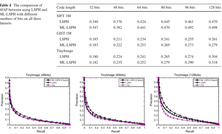
Table 4 The comparison of MAP between using LSPH and ML-LSPH with different numbers of bits on all three datasets

Code length 32 bits 48 bits 64 bits 80 bits 96 bits 128 bits SIFT 1M LSPH 0.340 0.376 0.424 0.445 0.461 0.470 ML-LSPH 0.347 0.382 0.441 0.470 0.492 0.498 GIST 1M LSPH 0.185 0.211 0.234 0.241 0.255 0.261 ML-LSPH 0.183 0.222 0.253 0.269 0.273 0.279 TinyImage LSPH 0.180 0.224 0.241 0.265 0.274 0.304 ML-LSPH 0.182 0.235 0.252 0.279 0.290 0.318 0 0.1 0.2 0.3 0.4 0.5 0.6 0.7 0.8 0.9 1 0 0.1 0.2 0.3 0.4 0.5 0.6 0.7 0.8 0.9 Recall Precision TinyImage (48bits) ML−LSPH (2 layers) LSPH ITQ 0 0.1 0.2 0.3 0.4 0.5 0.6 0.7 0.8 0.9 1 0 0.1 0.2 0.3 0.4 0.5 0.6 0.7 0.8 0.9 1 Recall Precision TinyImage (80bits) ML−LSPH (2 layers) LSPH ITQ 0 0.1 0.2 0.3 0.4 0.5 0.6 0.7 0.8 0.9 1 0 0.1 0.2 0.3 0.4 0.5 0.6 0.7 0.8 0.9 1 Recall Precision TinyImage (128bits) ML−LSPH (2 layers) LSPH ITQ

Fig. 9 Comparison of precision recall curves using ordinary LSPH (one layer) and ML-LSPH (two layers) with different bits on the TinyImage dataset (Color figure online)

0100 200 300 400 500 600 700 800 900 1000 0 0.005 0.01 0.015 0.02 0.025 0.03 0.035 0.04 0.045 0.05 Number of iterations Loss1 0100 200 300 400 500 600 700 800 900 1000 0 1 2 3 4 5 6 7x 10−3 Number of iterations Loss2 0100 200 300 400 500 600 700 800 900 1000 0 0.02 0.04 0.06 0.08 0.1 0.12 Number of iterations Total Loss (a) (b) (c) 0100 200 300 400 500 600 700 800 900 1000 0.237 0.238 0.239 0.24 0.241 0.242 0.243 0.244 0.245 0.246 0.247 Number of iterations Loss1 0100 200 300 400 500 600 700 800 900 1000 0 1 2 3 4 5 6 7 8x 10−3 Number of iterations Loss2 0100 200 300 400 500 600 700 800 900 1000 0.24 0.25 0.26 0.27 0.28 0.29 0.3 0.31 0.32 0.33 Number of iterations Total Loss (d) (e) (f)

Fig. 10 Illustration of convergence on the TinyImage dataset with the code length 64 (λ = 10). For ordinary LSPH (one layer): a loss1 = X −U₁V₁2 _{versus number of iterations. b loss2 =}

K L(P||Q) versus number of iterations. c T otalloss = X − U1V12+λK L(P||Q)versus number of iterations. For ML-LSPH:

dloss1 = X−g(U1g(U2· · ·g(UnVn)))2versus number of

iter-ations.eloss2 = n_i=1K L(P||Q(i)_{)versus number of iterations.f}

T otalloss= X−g(U1g(U2· · ·g(UnVn)))2+λni=1K L(P||Q(i)) versus number of iterations. Zoom in for better viewing

Meanwhile, the training and test time for all the methods are listed in Tables2and3, as well. Considering the training time, the random projection based algorithms are relatively more efficient, especially the LSH. While, RBM takes the most time for training, since it is based on a time-consuming deep learning method. Our method LSPH is significantly more efficient than STH, BSSC and RBM, but slightly slower than ITQ, AGH and SpH. It is noteworthy that once the opti-mal hashing functions of our method are obtained from the training phase, the optimized hashing functions will be fixed and directly used for new data. In addition, with the rapid development of silicon technologies, future computers will be much faster and even the training will become less a prob-lem. In terms of the test phase, LSH is the most efficient methods as well, since only a simple matrix multiplication and a thresholding are needed to obtain the binary codes. AGH and SpH always take more time for the test phase. Our LSPH has the competitive efficiency with STH. Therefore, in general, it can be concluded that LSPH is an effective and relatively efficient method for the large-scale retrieval tasks.

6.2 Evaluation on ML-LSPH

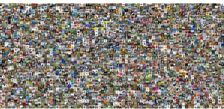
In this subsection, the multi-layer LSPH is evaluated on the TinyImage dataset, which is a subset containing 500,000

images5 from ***80 Million Tiny Images (Torralba et al.

2008a,b). Some example images from the TinyImage dataset

are illustrated in Fig. 6. We further take 1K images as

5_{This subset is downloaded fromhttp://groups.csail.mit.edu/vision/}

TinyImages/.

the queries by random selection and use the remaining to form the gallery database. Considering the cost of com-putation in multi-layer networks, in this experiment, only 100,000 randomly selected samples from the gallery data-base form the training set. Similar to the experiments of LSPH, another 50,000 data samples are also randomly cho-sen as a cross-validation set for parameter tuning. For image searching tasks, given an image, we describe it with 512-dimensional GIST descriptors (Oliva and Torralba 2001) in this experiment and then learn to hash these descriptors with all compared methods. In the querying phase, a returned point is regarded as a neighbor if it lies in the top ranked 500 points for the TinyImage dataset. We evaluate the retrieval results through Hamming distance ranking and report the Mean Average Precision (MAP) and the precision-recall curves by changing the number of top ranked points. Additionally, we also report the parameter sensitive analysis and visu-alize some retrieved images of compared methods on this dataset.

To avoid confusion, in this experiment, we only compare with LSH, PCAH, ITQ, AGH, RBM and SpH, which have shown distinctive performance according to the results in the previous comparison. Besides, we also add a new hashing technique SKLSH in this experiment. Note that, RBM here has 100-100-100 three hidden layers without fine-tuning. All of the above methods are then evaluated on six different lengths of codes (32, 48, 64, 80, 96, 128). Under the same experimental setting, all the parameters used in the compared methods have been strictly chosen according to their original papers.

For our ML-LSPH, the data zero-one normalization and hyper-parameter selection follow the same scheme as those in LSPH. Besides, to better reach the local minimum loss in ML-LSPH, the learning rateγ for iterative optimization is considered. In this experiment, we fixγ = 0.5 for ML-LSPH. More importantly, for the reason mentioned above that when the number of the layers increases, the accumu-lative reconstruction error will cause the non-convergence

problem of the proposed model (Trigeorgis et al. 2014),

we evaluate ML-LSPH with n = 2 layers, which is the

same setting as in Trigeorgis et al.(2014). We further set the dimension of the middle layer6(i.e.,V1) to 256 on this dataset.

6 _{After attempting various network architectures with different} dimen-sions of middle layers, the current ML-LSPH network is the best option for our task. Similar to the deep learning model (Krizhevsky et al. 2012;

Szegedy et al. 2014). It is noteworthy that the dimensions of middle lay-ers are quite sensitive to the data distribution (i.e., dataset) and there is no particular proof to explain what length of dimension for middle layers is better. Thus, we recommend to try different structure settings in order to determine what kind of structure can achieve the best performance.

0.08 0.1 0.12 0.14 0.16 0.18 0.2 0.22 0.24 0.26

Mean Average Precision

TinyImage (32 bits) ML−LSPH (2 layers) ITQ LSH ML−RBM (3 layers) 0.1 0.12 0.14 0.16 0.18 0.2 0.22 0.24 0.26 0.28 0.3

Mean Average Precision

TinyImage (48 bits) ML−LSPH (2 layers) ITQ LSH ML−RBM (3 layers) 0.16 0.18 0.2 0.22 0.24 0.26 0.28 0.3 0.32

Mean Average Precision

TinyImage (64 bits) ML−LSPH (2 layers) ITQ LSH ML−RBM (3 layers) 10−2 10−1 100 101 102 103 0.15 0.2 0.25 0.3 Value of λ 10−2 10−1 100 101 102 103 Value of λ

Mean Average Precision

TinyImage (80 bits) ML−LSPH (2 layers) ITQ LSH ML−RBM (3 layers) 0.15 0.2 0.25 0.3

Mean Average Precision

TinyImage (96 bits) ML−LSPH (2 layers) ITQ LSH ML−RBM (3 layers) 0.15 0.2 0.25 0.3

Mean Average Precision

TinyImage (128 bits) ML−LSPH (2 layers) ITQ LSH ML−RBM (3 layers) 10−2 ₁₀−1 ₁₀0 ₁₀1 ₁₀2 ₁₀3 Value of λ 10−2 10−1 100 101 102 103 Value of λ 10−2 ₁₀−1 ₁₀0 ₁₀1 ₁₀2 ₁₀3 Value of λ 10−2 10−1 100 101 102 103 Value of λ

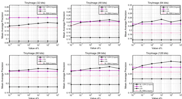
Fig. 11 Parameter sensitivity analysis of the regularization parameterλwith different bits on the TinyImage dataset (Color figure online)

Table 5 Results comparison (MAP) of ML-LSPH

with/without KL regularization termn_i=1K L(P||Q(i)₎

Code length 32 bits 48 bits 64 bits 80 bits 96 bits 128 bits With KL regularization term (λ=1) 0.174 0.224 0.242 0.273 0.280 0.305 Without KL regularization term (λ=0) 0.170 0.195 0.218 0.246 0.254 0.273

6.2.1 Results Comparison

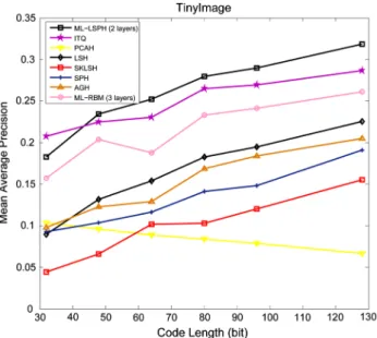
Fig.7illustrates the MAP curves of all compared algorithms on the TinyImage dataset. Our ML-LSPH algorithm achieves slightly lower MAP than ITQ when the code length is less than 48 bits but consistently outperforms all other compared methods in every length of code. RBM with 3 layers can also produce competitive search accuracies on this dataset. Dif-ferent to other hashing techniques, the performance of PCAH decreases with the increase of the code length. The similar phenomenon has appeared in the previous evaluation on SIFT 1M and GIST 1M datasets. The performance of AGH, SpH and LSH is consistent with that in the previous experiments. Besides, Fig.8shows a series of precision-recall curves with different code lengths on the TinyImage dataset with the 500 nearest neighbors as the ground truth. By comparing the Area Under the Curve (AUC), our ML-LSPH achieves apparently better performance than other methods on relatively long

bits (code length ≥ 48 bits) and the performance slightly

goes down when short hash codes are adopted. Moreover, in Table4and Fig.9, we also compare the performance between ML-LSPH and LSPH in terms of the MAP and AUC on all

three datasets. The ML-LSPH can achieve consistently better results than LSPH, since large intra-class variations in Tiny-Image cause complex and noisy data distributions, which are

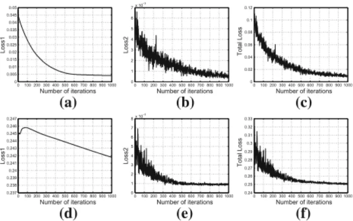
more difficult to handle by LSPH. Besides, Fig. 10

illus-trates the convergence of the proposed LSPH and ML-LSPH on TinyImage with the code length of 64. We can clearly observe that, for LSPH, the loss ofX−U1V12dramatically drops down when the number of iterations increases. While, for ML-LSPH, the loss ofX−g(U1g(U2· · ·g(UnVn)))2 first climbs up when the number of iterations is less than 50 and then goes down. With the batch-based learning scheme, the total losses of both LSPH and ML-LSPH can steadily decrease with little fluctuation.

Additionally, in Fig. 11, we also compare the retrieval performance of ML-LSPH with respect to the regularization parameterλalong different code lengths via cross-validation. When tuning the parameterλfrom 0.01 to 1000 with a scale factor of 10, the MAP curves of ML-LSPH appear to be rel-atively stable and insensitive to λ. For code lengths equal to 64 bits and 80 bits, the best performance occurs when λ=10. However, for the rest of the code lengths, ML-LSPH can achieve the highest retrieval accuracies withλ = 100.

Query images

(

a

)

(b)

(c)

(

d

)

(e)

(f)

(

g

)

(h)

Fig. 12 The top 25 retrieved images for queries (plane, bird, car, horse, ship and truck) with 96 bits using ML-RBM, LSH, SpH, PCAH, SKLSH, ITQ, AGH and our ML-LSPH (fromatoh). Best viewed in color (Color figure online)