Performance Evaluation of Completed Local Ternary Pattern (CLTP) for Face Image Recognition

Performance Evaluation of Completed Local Ternary

Pattern (CLTP) for Face Image Recognition

Sam Yin Yee

, Taha H. Rassem

, Mohammed Falah Mohammed

Faculty of Computer Systems and Software Engineering, Universiti Malaysia Pahang,

26300, Kuantan, Malaysia

Nasrin M. Makbol

College of Computer Science and Engineering Hodeidah University,

Hodeidah, Yemen

Abstract—Feature extraction is the most important step that affects the recognition accuracy of face recognition. One of these features are the texture descriptors that are playing an important role as local features descriptor in many of the face recognition systems. Recently, many types of texture descriptors had been proposed and used for face recognition task. The Completed Local Ternary Pattern (CLTP) is one of the texture descriptors that has been proposed for texture image classification and had been tested for different image classification tasks. It proposed to overcome the Local Binary Pattern (LBP) drawbacks where the CLTP is more robust to noise as well as shown a good discriminative property than others. In this paper, a comprehensive study on the performance of the CLTP for face recognition task has been done. The aim of this study is to investigate and evaluate the CLTP performance using eight different face datasets and compared with the previous texture descriptors. In the experimental results, the CLTP had been shown good recognition rates and outperformed the other texture descriptors for this task. Several face datasets are used in this paper, such as Georgia Tech Face, Collection Facial Images, Caltech Pedestrian Faces, JAFFE, FEI, YALE, ORL, UMIST datasets.

Keywords—Face recognition; recognition accuracy; Local Bi-nary Pattern (LBP); Completed Local BiBi-nary Pattern (CLBP); Completed Local Ternary Pattern (CLTP)

I. INTRODUCTION

Now-a-days, there are several ways for identifying a per-son. Much-advanced technology to recognize a person are voice recognition, fingerprint system, face recognition, and even iris pattern detection [1]. However, the friendliest and natural, lowest damage to verify a person is to use the face recognition. Moreover, it can be used to detect the facial expression of the person. The human brain has an ability to recognize a person face even she/he is wearing glasses, changing hairstyle or changing a facial expression or recognize the face after several years.

Face recognition is an image analysis that gained attention nowadays [2]. There are many algorithms has been proposed due to the importance of this field to achieve high recognition accuracy rates. Face recognition systems can be used in differ-ent fields such as security systems, attending systems, detect the criminal person in public place and checks the criminal record of someone. It would make a huge contribution in computer vision and is a success in the technology field. Face recognition plays an important role for identifying a person in compared with the others identification application. The identity of a person based on physiological characteristics can be recognized by the biometric approach of face recognition.

Since two decades, several feature descriptors are proposed and used face recognition such as texture, shape, color de-scriptors. Examples of texture descriptors that used for face recognition systems are the Local Binary Pattern (LBP) [3], Local Ternary Pattern (LTP) [4], Completed Local Binary Pattern (CLBP) [5], Colour Completed Local Binary Pattern (CCLBP) [6], Complated and Completed Local Ternary Pattern (CLTP) [7], [8]. The LBP was reported to be initially used for texture descriptors in 2002 [3]. The superiorities of LBP are bound to its invariance to revolution, robustness against monotonic dim level change, and also its low computational complexity. However, it has some disadvantages which high-sensitivity to noise as well as sometimes cannot distinguish different patterns [9]. These two problems have been men-tioned in many research papers as the drawbacks of LBP.

In spite of that, the Local Ternary Pattern (LTP) has been proposed to overcome the limitation of LBP which is more robust to noise comparing with LBP. However, the LTP sometimes cannot distinguish different patterns like the LBP. There are many texture descriptors have been proposed afterwards, such as CLBP, and CLTP.

The CLTP is proposed to be more robust to noise as well as more discriminative in comparison with the LBP, LTP and CLBP. For face recognition task, the performance of the CLTP had been evaluated and compared with other texture descriptors. However, only two face datasets were used in that evaluation study [9].

In this paper, we are collecting eight face datasets to evaluate the CLTP performance for face recognition. This is in order to have a deep investigation about the CLTP performance where different face datasets have challenges and different face properties. In this paper, the face recognition performance of CLTP is get evaluated with the different standard dataset. It used to compare with Completed Local Binary Pattern (CLBP) to extract the face image and showed a higher accuracy result than CLBP. In this study, the Georgia Tech Face, Collection Facial Images, Caltech Pedestrian Faces, JAFFE, FEI, YALE, ORL, UMIST datasets are used.

The present paper is organized as follows. Section II describes the related work in detail. Section III explains the proposed system. Section IV describes the experiment setup, Sections V and VI explain the experiment result and conclusions respectively.

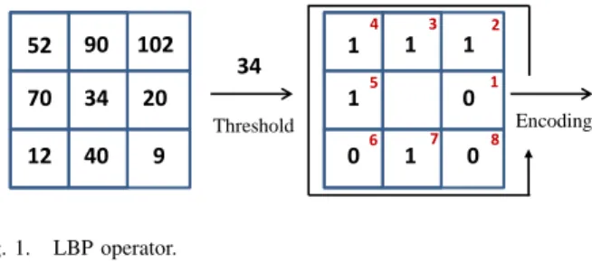
52 70 90 102 20 34 40 9 12 1 1 1 1 0 1 0 0 1 34 Threshold Encoding Binary 01111010 Decimal 122 2 3 4 5 6 7 8 Fig. 1. LBP operator.

II. RELATED WORK

In this section, the LBP, CLBP and CLTP are explained. A. Local Binary Pattern (LBP)

The initial LBP method proposed by Ojala et al. [3] was used to extract a texture feature. It provides the local measure of image contrast. LBP has initially been defined within the concept of 8 pixels and gray value centre pixel. The grey level variance between the centre pixel and its neighbourhood pixel is calculated. The neighbourhood pixels is set to 1 if the variance is positive or 0 if its negative; then, these values are used to obtain a binary code which is generated later to represent a histogram that describes the image texture. Fig. 1 shows the process of calculation in the original LBP.

The LBP descriptor was developed by Ojala et al. [10] based on the use of differently-sized neighbourhoods with the aid of a symmetric circle neighbourhood defined by R and P. The LBP is defined as:

LBPP,R = P−1 X p=0 2ps(ip−ic), s(x) = 1, x≥0, 0, x <0, (1)

whereic denotes the gray value of the centre pixel in the

pattern, ip(p = 0, . . . , P −1) denotes the gray values of the

neighbour pixel on a circle of radius R. While P denotes the number of neighbours.

In LBP, the bilinear interpolation estimation method is used to identify the neighbours that do not lie in the exact centre of the pixels.

B. Completed Local Binary Pattern (CLBP)

The CLBP is proposed as extension of LBP in 2010 by Guo et al. [5]. The CLBP becomes one of the successful texture descriptors. The CLBP operator is consist of three different parts which are CLBP S, CLBP M and CLBP C.

Firstly, each pattern in the image is decomposed into two complementary components, namely, the sign component sp

and the magnitude component mp which can be

mathemati-cally expressed as follows.

sp=s(ip−ic), mp=|ip−ic| (2)

Then, the sp and mp are used to construct CLBP S and

CLBP M, respectively. The mathematical expression of CLBP S is as follows: CLBP SP,R = P−1 X p=0 2ps(ip−ic), sp= 1, ip≥ic, 0, ip< ic, (3) whereic,ip,R, andP are defined in (1), whilec denotes the

mean value of mp in the entire image.

The following component is CLBP M which proceeds with qualities rather than binary values. The neighbourhoods pixel will change to 1 if the difference between their value and mean of the pattern is positive. Otherwise, it will change to 0. CLBP M is shown in the following equation.

CLBP MP,R = P−1 X P=0 2Pt(mp−c) , t(mp, c) = 1, |ip−ic| ≥c 0, |ip−ic|< c (4)

where ic donates the middle pixel, and P is uniformly

dispersed neighbours which is ip, and mp is the mean value

of the whole image. Example of CLBP extraction is shown in Fig. 2.

Fig. 2. Difference between sign components and magnitude components. (a) 3*3 sample block, (b) Local differences, (c) Sign components, (d) Magnitude components (mean = 22), (e) Final magnitude components.

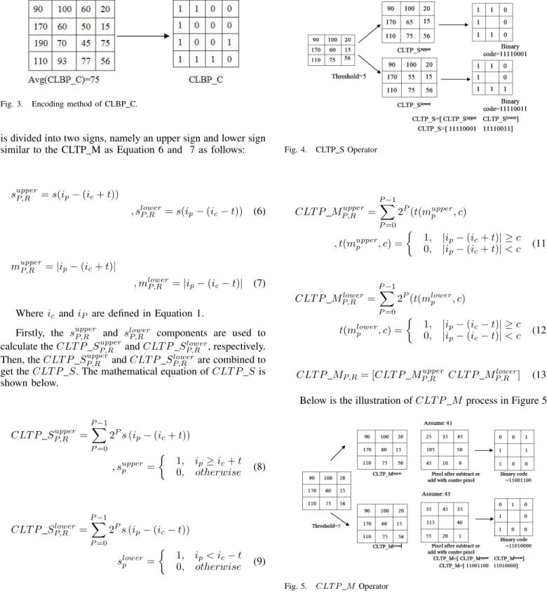
Lastly, Guo et al. utilized the estimation of the grey level of the image to build CLBP-Centre (CLBP C). The CLBP C can be described scientifically as Equation 5.

CLBP CP,R=t(ip−cI) (5)

Where cI is the threshold that can be calculated as the

mean of the grey level of the picture. Therefore, the CLBP is very useful in extracting the rotation invariant uniform into a binary pattern which helps in removing the pivot invariant uniform element in the face. Fig. 3 shows the illustration of CLBP C.

C. Completed Local Ternary Pattern (CLTP)

Completed Local Ternary Pattern (CLTP) had been pre-sented by Rassem and Khoo (2014) for rotation invariant texture classification. CLTP is proposed to overcome the drawbacks of the LBP as well as the CLBP [8]. The CLTP S

Fig. 3. Encoding method of CLBP C.

is divided into two signs, namely an upper sign and lower sign similar to the CLTP M as Equation 6 and 7 as follows:

supper_P,R =s(ip−(ic+t))

, slower_P,R =s(ip−(ic−t)) (6)

mupper_P,R =|ip−(ic+t)|

, mlower_P,R =|ip−(ic−t)| (7)

Whereic andiP are defined in Equation 1.

Firstly, the supper_P,R and slower

P,R components are used to

calculate theCLT P S_P,RupperandCLT P Slower

P,R , respectively.

Then, theCLT P S_P,RupperandCLT P Slower

P,R are combined to

get theCLT P S. The mathematical equation ofCLT P S is shown below. CLT P S_P,Rupper= P−1 X P=0 2Ps(ip−(ic+t)) , supper_p = 1, ip≥ic+t 0, otherwise (8) CLT P S_P,Rlower= P−1 X P=0 2Ps(ip−(ic−t)) slowerp = 1, ip< ic−t 0, otherwise (9) CLT P SP,R= [CLT P S upper P,R CLT P S lower P,R ] (10)

The illustration ofCLT P S process is shown in Figure 4.

CLT P M is similar to the CLT P S which needs to add the CLT P M_P,Rupper and CLT P Mlower

P,R to get the

CLT P MP,R. The output of CLT P M also will be in a

binary form same with CLT P S as shown below:

Fig. 4. CLTP S Operator CLT P M_P,Rupper= P−1 X P=0 2P(t(mupper_p , c) , t(mupper_p , c) = 1, |ip−(ic+t)| ≥c 0, |ip−(ic+t)|< c (11) CLT P M_P,Rlower = P−1 X P=0 2P(t(mlower_p , c) t(mlower_p , c) = 1, |ip−(ic−t)| ≥c 0, |ip−(ic−t)|< c (12) CLT P MP,R= [CLT P MP,Rupper CLT P M lower P,R ] (13)

Below is the illustration ofCLT P M process in Figure 5.

Fig. 5. CLT P MOperator

The outcome of CLT P C is a 2D matrix of the binary value. It compares the average pixel number of the origi-nal pixel number with the upper and lower of CLT P C component. Then it comes out with a 2D matrix of binary value of CLT P C_P,Rupper and 2D matrix of binary value of CLT P C_P,Rlower, the mathematical method is shown as Equa-tion 14 and 15 below:

CLT P C_P,Rlower=t(ilower_p , cI) (15)

The final CLT P CP,R can be obtained as shown in the

following Equation. CLT P SP,R= [CLT P S upper P,R CLT P S lower P,R ] (16)

The illustrator of CLT P Cas shown in below Fig. 6.

Fig. 6. CLT P COperator.

III. PROPOSEDSYSTEM

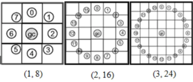
The face recognition has a very complex process and it extremely contrasts from others in different aspects. Thus, the improvement for face recognition system will be a troublesome undertaking in image processing of computer vision. A radius size is allocated to carry out the extraction process in the earlier stage of feature extraction. The ranges of radius sizes have many sets, of which the widely recognized sets used are (1, 8), (2, 16) and (3, 24), These radius sizes can become an arrangement of various outcome as shown in Fig. 7.

Fig. 7. The illustration of radius sizes.

First, a set of training and testing images are prepared and processed for feature detection. Once the feature of the image is detected, the feature extraction stage applies the CLTP feature descriptor to the image. The feature extraction stage is the process to extract the CLTP texture of each image i.e., training and testing images. After proceeding with the feature extraction, the similarity training images features are grouped together. The familiar image in the testing will be compared with all the extracted features image in training image to find the smallest distance or closest value between the training and testing image features. General face recognition structure is shown in Fig. 8.

Fig. 8. General face recognition structure.

IV. EXPERIMENTSETUP

In the performance evaluation, to check the effectiveness of the CLBP and CLTP descriptors, different datasets had been used in the experiments with different training images numbers. The training images are select randomly from every individual, and the remaining images will be used for testing images. For different datasets, the step is repeat 100 times to choose different training samples and calculate the average recognition rate. Due to the large dimension of the Caltech Pedestrian Faces 1999 [11] dataset images, they had been cropped to 60 x 60 images size to execute the experiment, while others dataset remains the same sizes. The face recog-nition performance of CLBP and CLTP on different datasets are tested and recorded. The outcomes are shown in Tables I to VIII for the datasets of JAFFE [12], UMIST [13], ORL [12], YALE [14], Collection Facial Images [15], Georgia Tech Face [16], Caltech Pedestrian Faces Dataset 1999 [11] and FEI [17], respectively.

V. EXPERIMENTRESULT

A. Japanese Female Facial Expressions Dataset (JAFFE) JAFFE dataset [18] comprised 213 faces images from 10 different classes of Japanese female in Japan. The features extraction of (1, 8), (2, 16) and (3, 24) radius sizes based on 2, 5 and 10 random choose of training images from the classes were used. Each class has 20 JPEG images with a different view of facial expression including angry, smile, sad, worry, nervous, neutral and others. The size of each image is 256 x 256. Example of some images of JAFFE is shown in Fig. 9.

Fig. 9. Some images from JAFFE dataset

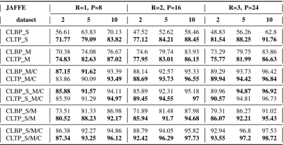
As shown in Table I, the classification result ofCLT P is higher rate than CLBP with all different pattern sizes using different number of training images. The CLT PS/M/C3,4

achieved highest classification rate, reaches 98.72% while the CLBPS/M/C3,4 achieved 97.53%.

TABLE I. CLASSIFICATIONACCURACY ONJAFFEDATASET(JAFFE) JAFFE R=1, P=8 R=2, P=16 R=3, P=24 dataset 2 5 10 2 5 10 2 5 10 CLBP S 56.61 63.83 70.13 47.52 52.62 58.46 48.83 56.26 62.8 CLTP S 71.77 79.09 83.82 77.12 84.21 88.45 81.54 88.25 91.76 CLBP M 70.38 74.08 76.67 74.6 79.74 83.93 73.29 79.75 83.86 CLTP M 74.83 82.63 87.02 77.95 83.01 86.15 75.77 81.99 86.63 CLBP M/C 87.15 91.62 93.39 88.14 92.57 95.33 89.29 93.73 96.42 CLTP M/C 83.86 90.09 93.49 88.69 93.73 96.55 89.94 94.42 96.84 CLBP S M/C 85.88 91.57 94.11 85.89 92.31 95.18 89.96 94.87 96.92 CLTP S M/C 85.59 91.29 94.97 89.45 94.55 97 90.57 94.81 96.73 CLBP S/M 73.51 81.33 86.98 71.89 81.48 87.98 79.31 86.27 91.02 CLTP S/M 80.52 88.23 92.17 85.94 91.7 94.68 86.07 92.21 95.43 CLBP S/M/C 86.38 92.27 94.86 88.79 94.05 95.82 92.94 96.8 97.53 CLTP S/M/C 87.34 93.25 96.12 92.42 96.29 97.73 93.55 97.2 98.72

B. Sheffield Face Dataset (UMIST)

UMIST dataset [13] contains 564 images from 20 indi-vidual classes. Each class has a different number of images. The biggest class has 48 images. Different training number has been selected from each class; 8, 13 and 19, while the remaining images are used for testing. Each individual has captured with a different view of the angle of the face. Some images of the UMIST dataset are shown in Fig. 10.

Fig. 10. Some images from UMIST dataset.

The result of UMUIST dataset on N = (8, 13, 19) is presented in Table II. The CLT P S/M/C3,24 has showed

99.68% of face recognition classification rate while the CLBPS/M/C3,4achieved 99.55%. In some cases, theCLBP

showed better results than CLTP, especially with small pattern size (1, 8) and (2, 16). While with (3, 24), the CLTP was better than CLBP with different number of training images. C. ORL Face dataset (ORL)

ORL face dataset [12] comprises of 400 pictures of 40 classes, they capture their images under various lighting con-dition, times, outward appearance and facial points of interest. In each class, N=(2, 5, 8) images are selected randomly for training images, others are used for testing images. Fig. 11 shows some images of ORL datasets.

Fig. 11. Some images from ORL dataset.

In ORL dataset, CLT P S/M/C3,24 achieved the best

classification rate result 98.52%. The best results by CLBP

was 97.98%. The CLTP outperformed the CLBP with different number of training image as well as with different texture pat-tern except in (1,8) where the CLBP S/M/C1,8 performed

better thanCLT P S/M/C1,8. The full experiment results are

shown in Table III.

D. YALE Face dataset (YALE)

YALE dataset [14] has captured by 15 people, every people are requested to capture 11 images so that it contains 165 images in the whole dataset. Each image is captured from alternate points of view, with a big difference in brightening and face expression. In this project, each picture in the YALE dataset was physically trimmed follow the face detected point sizes. In each class, N=(2, 5, 10) images are used for training while the remaining for testing. Some images from the dataset are shown in Fig. 12.

Fig. 12. Some images from YALE dataset.

Table IV shows the classification rates using CLBP and CLTP. As shown in the table, the CLTP outperformed the CLBP with different pattern texture size as well as using dif-ferent training images’ numbers. The best result is achieved by CLT P S/M/C3,24, reaches 80.47% compared with 77.20%

achieved byCLBP S/M/C3,24.

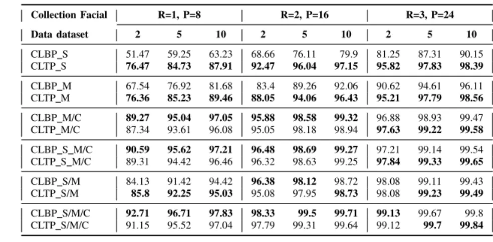
E. Collection Facial Images dataset

Collection Facial Images dataset [15] includes 152 classes. Each class has 20 different images with a size of 180 x 200. This dataset consists of various faces, most of them were undergraduate students between 18 to 20 years old. This dataset only has a slightly different facial expression so that the accuracy of face recognition would be higher than other datasets. In each class, N =(2, 5, 10) images are used for training while the remaining for testing.

In Collection Facial Images dataset, The CLT P S/M/C3,24 achieved 99.84% accuracy rate

TABLE II. CLASSIFICATIONACCURACY ONSHEFFIELDFACE DATASET(UMIST) UMIST R=1, P=8 R=2, P=16 R=3, P=24 dataset 8 13 19 8 13 19 8 13 19 CLBP S 55.77 61.06 65.4 64.39 72.33 79.36 72.13 80.75 87.44 CLTP S 69.8 79.06 85.08 78.96 88.42 93.7 85.63 93.29 97.43 CLBP M 67.6 74.07 79.03 70.65 76.93 82.23 75.91 83.26 87.13 CLTP M 79.76 86.17 89.85 89.72 93.52 95.78 93.03 97.16 98.31 CLBP M/C 90.29 94.69 97.01 92.11 96.24 97.76 93.15 96.79 98.19 CLTP M/C 90.6 94.93 96.68 96.36 98.79 99.41 96.8 99.15 99.24 CLBP S M/C 91.49 96.1 98.2 94.42 98.35 99.39 95.5 98.88 99.54 CLTP S M/C 92.98 96.71 97.98 96.45 98.88 99.47 96.67 99.32 99.32 CLBP S/M 88.77 94.4 97.31 93.58 97.49 98.74 95.9 98.43 99.27 CLTP S/M 90.63 95.09 96.71 94.96 98.2 99.1 95.98 99.05 99.54 CLBP S/M/C 95.69 98.34 99.08 97.79 99.47 99.54 98.12 99.5 99.55 CLTP S/M/C 95.36 98.11 98.53 97.73 99.45 99.53 97.88 99.57 99.68

TABLE III. CLASSIFICATIONACCURACY ONORL FACE DATASET(ORL)

ORL R=1, P=8 R=2, P=16 R=3, P=24 dataset 2 5 8 2 5 8 2 5 8 CLBP S 26.89 31.42 33.74 42.15 52.3 55.49 51.58 63.27 68.71 CLTP S 53.36 70.19 77.11 65.92 83.21 88.85 71.23 87.74 91.7 CLBP M 43.43 54.02 59.81 56.55 67.5 70.7 60.45 74.05 79.39 CLTP M 48.11 65.53 72 63.93 80.68 85.63 70.35 85.68 90.53 CLBP M/C 64.74 79.92 84.84 69.65 86.29 91.18 70.8 88.1 94.15 CLTP M/C 65.64 83.39 89.54 76.01 92.83 96.84 79.05 94.35 97.74 CLBP S M/C 68.55 83.86 89.1 73.93 89.58 94.35 77.06 91.98 95.7 CLTP S M/C 69.2 87.28 92.55 78.46 93.58 97.14 81.34 94.97 98.01 CLBP S/M 66.87 81.1 86.34 76.39 90.2 94.64 80.22 92.46 95.79 CLTP S/M 68.53 86.11 91.2 77.9 91.81 96.25 81.75 95.14 98.21 CLBP S/M/C 79.5 93.37 97.3 83.08 95.34 97.66 84.57 95.98 97.98 CLTP S/M/C 75.71 92.06 95.85 84.76 95.91 98.31 86.98 97.08 98.52

TABLE IV. CLASSIFICATIONACCURACY ONYALE FACE DATASET(YALE)

YALE R=1, P=8 R=2, P=16 R=3, P=24 dataset 2 5 10 2 5 10 2 5 10 CLBP S 41.4 50.16 53.93 37.24 45.83 54.67 41.24 52.36 62.6 CLTP S 43.59 54.64 57.67 47.78 58.83 64 53.2 62.32 70.4 CLBP M 44.36 50.34 56.13 48.22 57.49 64.07 49.9 58.72 63.33 CLTP M 53.02 60.94 64.73 54.24 66.53 67.13 61.05 70.09 74.07 CLBP M/C 60.78 68.43 70.8 60.16 69.44 66.93 62.5 70.63 72.47 CLTP M/C 59.33 67.87 68.93 64.19 73.88 77.87 66.13 72.98 76.4 CLBP S M/C 57.25 65.06 69.27 55.02 66.07 69.6 59.68 69 71.4 CLTP S M/C 60 67.04 70.73 64.09 72.98 71.6 66.57 73.93 73.73 CLBP S/M 51.5 61.87 64.93 52.64 65.66 73.6 60.36 69.82 75.4 CLTP S/M 57.64 67.11 67.87 61.03 72.22 74 64.16 73.52 74.4 CLBP S/M/C 59.9 71.33 70.33 58.96 70.3 77.07 64.21 75.31 77.2 CLTP S/M/C 61.81 69.86 74.93 68.99 74.78 76.53 70.49 76.58 80.47

Fig. 13. Some images from Collection Facial Images dataset.

CLBP S/M/C3,24. Table V shows that the CLTP with

better than CLBP with big texture pattern size (3,24) while the performance with (1,8) and (2,16) was depending on the combination of the operators in CLBP and CLTP.

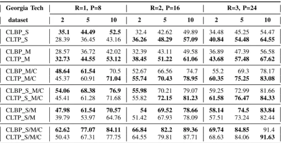
F. Georgia Tech Face dataset

The Georgia Tech Face dataset [16] contains 50 and class contains exactly 15 samples of colour images with a size of 141 x 216 captured in 1999. The images show the front of the face with different expressions, scale and illumination condition. Besides that, some of the faces in this dataset wearing spectacles and some photos in small size and with a low-resolution. In each class, N =(2, 5, 10) images are used for training while the remaining for testing. Fig. 14 shows some examples of Georgia Tech Face images.

TABLE V. CLASSIFICATIONACCURACY ONCOLLECTIONFACIALIMAGES DATASET Collection Facial R=1, P=8 R=2, P=16 R=3, P=24 Data dataset 2 5 10 2 5 10 2 5 10 CLBP S 51.47 59.25 63.23 68.66 76.11 79.9 81.25 87.31 90.15 CLTP S 76.47 84.73 87.91 92.47 96.04 97.15 95.82 97.83 98.39 CLBP M 67.54 76.92 81.68 83.4 89.26 92.06 90.62 94.61 96.11 CLTP M 76.36 85.23 89.46 88.05 94.06 96.43 95.21 97.79 98.56 CLBP M/C 89.27 95.04 97.05 95.88 98.58 99.32 96.88 98.93 99.47 CLTP M/C 87.34 93.61 96.08 95.05 98.18 98.94 97.63 99.22 99.58 CLBP S M/C 90.59 95.62 97.21 96.48 98.69 99.27 97.21 99.14 99.54 CLTP S M/C 89.31 94.42 96.46 96.32 98.63 99.25 97.84 99.33 99.65 CLBP S/M 84.13 91.42 94.42 96.38 98.12 98.72 98.08 99.11 99.43 CLTP S/M 85.8 92.25 95.03 95.08 97.95 98.73 98.08 99.23 99.49 CLBP S/M/C 92.71 96.71 97.83 98.33 99.5 99.71 99.13 99.67 99.8 CLTP S/M/C 91.15 95.52 97.04 97.79 99.31 99.64 99.12 99.7 99.84

Fig. 14. Some images from Georgia Tech Face dataset.

with 91.63%. CLTP result work better in the larger texture pat-tern size (R=3, P=24). While, the CLBP achieved better with texture pattern (1,8) with different image training numbers. In (2,16), the CLTP was better in some cases and less than CLBP in another cases.

G. Caltech Pedestrian Faces Dataset 1999

The Caltech Pedestrian Faces Dataset 1999 was down-loaded from online sources [11] collected at California Institute of Technology consisting of 380 face images with 19 identities classes were used in this experiment. Every class contains 20 JPEG images with different angle view of the face, face expression background and lighting. This dataset images size is 896 x 592. In each class, N =(2, 5, 10) images are used for training while the remaining for testing. Examples of Caltech Pedestrian Faces images are shown in Fig. 15.

Fig. 15. Some images from Caltech Pedestrian Faces Dataset 1999.

Table VII shows the classification accuracy for CALTECH using CLBP and CLTP. The performance of CLTP is better work in the Caltech Pedestrian Faces Dataset 1999 compare the CLBP. This can see that majority result of CLTP is higher than CLBP on different texture pattern sizes and training images. CLTP achieved 78.78% as the best accuracy results while CLBP achieved 76.57%.

H. FEI Face dataset

The FEI face dataset [17] is a dataset of faces collected at Brazil. This dataset has 200 faces of Brazilian people captured in 2005 and 2006 at Artificial Intelligence Laboratory of FEI

in S˜ao Bernardo do Campo, S˜ao Paulo, Brazil. FEI face dataset has 2800 face images from students and staffs in the FEI from 19 years old to 40 years old. In 200 classes, there were 14 images from every class which contain different degree view with the profile rotation of almost 180 degrees and with different facial expression. The size of faces image was in 640 x 480 pixels. Examples of some images from FEI face dataset are shown in Fig. 16.

Fig. 16. Some images from FEI Face dataset.

The result classification of FEI face dataset with various radius sizes is shown in Table VIII. The CLT P S/M/C3,24

achieved highest classification rate, reaches 76.38% while 75.48% achieved by CLBP. Table VIII shows the full experi-ment results of CLBP and CLTP with different training images as well as under texture pattern sizes. The result table shows that the CLTP outperformed the CLBP in many cases.

In general, the summary of the classification accuracy results of all benchmark datasets are shown in Table IX. The results showed the priority of the CLTP performance against the CLBP. The CLTP achieved the best in all datasets compared with CLBP.

VI. CONCLUSION

Completed Local Ternary Pattern (CLTP) is one of the new texture descriptors that is proposed to overcome the drawbacks of the LBP. In this paper, we applied the CLTP for face image classification task. The performances of CLTP as well as CLBP were studied and evaluated using eight different benchmark datasets. The experiment results show that the CLTP achieved the highest classification rates compared with CLBP. The CLTP outperformed CLBP performance under different pattern sizes and using a different number of training images. The CLTP good performance is due to its robustness to noise than CLBP. In addition, CLTP has more discriminating property than CLBP. In future work, the CLTP can be combined with other descriptors such as CLBP. This combination will help

TABLE VI. CLASSIFICATIONACCURACY ONGEORGIATECH DATASET Georgia Tech R=1, P=8 R=2, P=16 R=3, P=24 dataset 2 5 10 2 5 10 2 5 10 CLBP S 35.1 44.49 52.5 32.4 42.62 49.89 34.48 45.25 54.47 CLTP S 28.39 36.45 43.16 36.26 48.29 57.09 40.84 54.48 64.55 CLBP M 28.57 36.72 42.02 32.39 43.11 49.58 36.89 47.39 56.58 CLTP M 32.73 44.55 53.12 38.45 51.22 61.06 43.68 57.48 67.62 CLBP M/C 48.64 61.54 70.5 52.67 66.56 74.7 55.2 69.3 78.17 CLTP M/C 45.37 60.91 71.04 55.74 70.43 78.95 60.35 75.25 83.08 CLBP S M/C 54.06 68.38 76.9 55.98 70.21 79.07 59.25 72.99 81.66 CLTP S M/C 45.41 61.28 71.68 55.82 72.15 81.23 61.58 76.47 84.33 CLBP S/M 47.98 61.54 70.57 54 69.52 78.66 58.14 74.5 83.84 CLTP S/M 39.79 53.97 64.76 51.42 67.93 78.09 57.51 73.24 82.44 CLBP S/M/C 62.62 77.07 84.11 66.84 82.2 89.36 69.74 84.85 91.4 CLTP S/M/C 50.43 67.31 77.75 64.55 79.81 87.71 68.63 84.06 91.63

TABLE VII. CLASSIFICATIONACCURACY ONCALTECHPEDESTRIANFACES1999DATASET Caltech Pedestrian R=1, P=8 R=2, P=16 R=3, P=24 Faces 1999 dataset 2 5 10 2 5 10 2 5 10 CLBP S 22.69 23.55 23.34 30.82 34.35 36.06 35.65 49.19 59.62 CLTP S 36.11 41.23 43.52 43.95 52.04 56.3 33.12 43.54 52.36 CLBP M 25.62 26.58 27.79 35.51 40.49 44.48 43.14 49.84 52.16 CLTP M 36.85 41.24 44.31 44.38 51.76 57.05 55.34 64.17 68.17 CLBP M/C 35.52 40.58 42.68 43.19 50.96 55.05 43.66 50.34 54.59 CLTP M/C 49.35 56.08 59.96 53.67 64.55 70.2 55.98 63.41 68.96 CLBP S M/C 43.1 47.71 50.34 51.91 61.22 64.69 51.46 60.39 64.97 CLTP S M/C 51.99 59.46 64.32 58.35 68.44 73.03 59.51 69.34 74.69 CLBP S/M 37.65 42.4 47.97 49.32 57.34 62.16 60.63 69.14 74.06 CLTP S/M 50.46 55.79 59.86 59.88 69.25 74.23 65.94 73.66 77.53 CLBP S/M/C 50.09 55.45 61.27 53.1 62.31 69.17 63.06 71.78 76.57 CLTP S/M/C 56.79 64.95 70.01 57.13 67.26 73.28 65.33 74.15 78.78

TABLE VIII. CLASSIFICATIONACCURACY ONFEIDATASET

FEI dataset R=1, P=8 R=2, P=16 R=3, P=24 2 5 10 2 5 10 2 5 10 CLBP S 12.38 16.77 20.82 9.02 12.06 14.86 11.99 16.29 20.07 CLTP S 28.22 36.31 42.37 39.52 51.75 61.03 41.92 56.08 65.8 CLBP M 19.17 26.29 32.78 23.77 32.59 40.14 26.64 36.8 45.67 CLTP M 22.98 31.06 37.59 24.51 33.4 40.83 23.16 32.53 41.3 CLBP M/C 33.04 46.15 55.33 36.8 49.94 58.24 39.23 53.2 64.2 CLTP M/C 38.28 52.06 60.38 41.23 55.01 63.5 36.77 51.33 63.01 CLBP S M/C 32.63 43.96 51.64 37.45 50.22 57.91 43.39 57.05 66.98 CLTP S M/C 43.61 57.33 65.67 46.93 61.26 69.33 43.55 58.52 68.83 CLBP S/M 22.79 33.68 42.89 29.5 41.97 51.77 40.55 55.16 63.62 CLTP S/M 39.46 54.52 65.01 44.31 59.57 69.39 42.13 57.93 67.52 CLBP S/M/C 37.2 50.91 60.46 45.98 60.55 70.71 53.88 68.94 75.48 CLTP S/M/C 50.83 65.34 72.91 53.8 68.65 75.4 51.16 67.4 76.38

TABLE IX. CLASSIFICATION ACCURACY ON BENCHMARK DATASETS

dataset Reference Classes Size CLBP CLTP

1 JAFFE [18] 10 256 x 256 97.53% 98.72%

2 ORL [12] 20 60 x 60 97.98% 98.52%

3 UMIST [13] 40 112 x 92 99.55% 99.68%

4 Yale [14] 15 153 x 153 77.20% 80.47%

5 Collection Facial Images [15] 152 180 x 200 99.80% 99.84%

6 Georgia Tech Face [16] 50 141 x 216 91.40% 91.63%

7 Caltech Pedestrian Faces 1999 [11] 19 60 x 60 76.57% 78.78%

to improve the classification accuracy rates in the face image classification task.

ACKNOWLEDGMENT

This research has been supported by Universiti Malaysia Pahang (UMP) Grant Number RDU180365.

REFERENCES

[1] I. Nurtanio, E. R. Astuti, I. K. E. Purnama, M. Hariadi, and M. H. Purnomo, “Classifying cyst and tumor lesion using support vector machine based on dental panoramic images texture features,”IAENG International Journal of Computer Science, vol. 40, no. 1, pp. 29–37, 2013.

[2] Z. Xia, C. Yuan, X. Sun, D. Sun, and R. Lv, “Combining wavelet transform and LBP related features for fingerprint liveness detection,” IAENG International Journal of Computer Science, vol. 43, no. 3, pp. 290–298, 2016.

[3] T. Ojala, M. Pietik¨ainen, and D. Harwood, “A comparative study of texture measures with classification based on featured distributions,” Pattern recognition, vol. 29, no. 1, pp. 51–59, 1996.

[4] X. Tan and B. Triggs, “Enhanced local texture feature sets for face recognition under difficult lighting conditions,” IEEE transactions on image processing, vol. 19, no. 6, pp. 1635–1650, 2010.

[5] Z. Guo, L. Zhang, and D. Zhang, “A completed modeling of local binary pattern operator for texture classification,”IEEE Transactions on Image Processing, vol. 19, no. 6, pp. 1657–1663, 2010.

[6] T. H. Rassem, B. E. Khoo, N. M. Makbol, and A. A. Alsewari, “Multi-scale colour completed local binary patterns for scene and event sport image categorisation.”IAENG International Journal of Computer Science, vol. 44, no. 2, 2017.

[7] T. H. Rassem and B. E. Khoo, “Completed local ternary pattern for rotation invariant texture classification,” The Scientific World Journal, vol. 2014, 2014.

[8] T. H. Rassem, M. F. Mohammed, B. E. Khoo, and N. M. Makbol, “Performance evaluation of completed local ternary patterns (CLTP) for medical, scene and event image categorisation,” in2015 4th Inter-national Conference on Software Engineering and Computer Systems (ICSECS). IEEE, 2015, pp. 33–38.

[9] T. H. Rassem, N. M. Makbol, and S. Y. Yee, “Face recognition using completed local ternary pattern (CLTP) texture descriptor,” Interna-tional Journal of Electrical and Computer Engineering (IJECE), vol. 7, no. 3, pp. 1594–1601, 2017.

[10] T. Ojala, M. Pietikainen, and T. Maenpaa, “Multiresolution gray-scale and rotation invariant texture classification with local binary patterns,” IEEE Transactions on Pattern Analysis and Machine Intelligence, vol. 24, no. 7, pp. 971 –987, jul 2002.

[11] (May 25th, 2018) Caltech face dataset. [Online]. Available:

www.vision.caltech.edu/ImageDatasets/f aces/f aces.tar/ [12] F. S. Samaria and A. C. Harter, “Parameterisation of a stochastic model

for human face identification,” in Applications of Computer Vision, 1994., Proceedings of the Second IEEE Workshop on. IEEE, 1994, pp. 138–142.

[13] D. B. Graham and N. M. Allinson, “Characterising virtual eigensigna-tures for general purpose face recognition,” in Face Recognition. Springer, 1998, pp. 446–456.

[14] P. N. Belhumeur, J. P. Hespanha, and D. J. Kriegman, “Recognition using class specific linear projection,” 1997.

[15] (2008) Collection of facial images. 2008. [Online]. Available: http://cswww. essex. ac. uk/mv/allfaces/index. htmlr

[16] A. Nefian and M. H. Hayes III, “A hidden markov model-based ap-proach for face detection and recognition,” Ph.D. dissertation, School of Electrical and Computer Engineering, Georgia Institute of Technology, 1999.

[17] C. E. Thomaz and G. A. Giraldi, “A new ranking method for principal components analysis and its application to face image analysis,”Image and Vision Computing, vol. 28, no. 6, pp. 902–913, 2010.

[18] M. J. Lyons, J. Budynek, and S. Akamatsu, “Automatic classification of single facial images,” IEEE transactions on pattern analysis and machine intelligence, vol. 21, no. 12, pp. 1357–1362, 1999.