Multivariate skew t mixture models: applications to fluorescence-activated cell sorting data

(1)

Multivariate skew t mixture models: Applications to

fluorescence-activated cell sorting data

Kui Wang Department of Mathematics University of Queensland St. Lucia, Q4072, Australia Email: [email protected] Shu-Kay Ng School of Medicine Griffith University (Logan Campus)

Meadowbrook, Q4131, Australia Email: [email protected] Geoffrey J McLachlan Department of Mathematics University of Queensland St. Lucia, Q4072, Australia Email: [email protected]

Abstract—In many applied problems in the context of pattern recognition, the data often involve highly asymmetric observations. Normal mixture models tend to overfit when additional components are included to capture the skewness of the data. Increased number of pseudo-components could lead to difficulties and inefficiencies in computations. Also, the contours of the fitted mixture components may be distorted. In this paper, we propose to adopt mixtures of multivariate skew t distributions to handle highly asymmetric data. The EM algorithm is used to compute the maximum likelihood estimates of model parameters. The method is illustrated using a flurorescence-activated cell sorting data.

Keywords-Asymmetric multivariate data; EM algorithm; fluorescene-activated cell sorting; mixture models; skewed t.

I. INTRODUCTION

Finite mixture models have been extensively developed and widely applied to density estimation and pattern recog-nition problems [1], [2], [3], [4]. With this approach to pat-tern recognition, the observedp-dimensional feature vectors

y1, . . . ,yn are assumed to have come from a mixture of a finite number, sayg, of groups in some unknown proportions π₁, . . . , πg that sum to one. That is, each feature vector yj

is taken to be a realization of the mixture probability density function (p.d.f.) defined by f(y;Ψ) = g i=1 πif(yj;θi), (1)

where f(yj;θi) denotes the ith component density with unknown parameter vector θi (i = 1, . . . , g). The compo-nent distributions are usually specified to belong to the same parametric family. Here the vectorΨof unknown parameters consists of the mixing proportions π1, . . . , πg−1 and the elements of theθiknown a priorito be distinct. The fitting of finite mixture models (1) can be obtained by maximum likelihood via the expectation-maximization (EM) algorithm of Dempster, Laird, and Rubin [5]; see also [6]. Frequently, in practice, it is reasonable to consider fitting mixtures of elliptically symmetric component densities. Within this class of component densities, the multivariate normal density is

a convenient choice given its computational tractability [1]. In applications where the tails of the normal distribution are shorter than appropriate or the parameter estimates are affected by atypical observations (outliers), the fitting of mixtures of multivariate t-distributions provides a more robust approach to the fitting of normal mixture models [7]. The t component density with location parameter μi, positive-definite matrix Σi, and νi degrees of freedom is given by tp(yj;μi,Σi, νi) = Γ(νi+p 2 )|Σi|−1/2 (πνi) 1 2pΓ(νi 2){1 +δ(yj,μi;Σi)/νi} 1 2(νi+p) , (2) where

δ(yj,μi;Σi) = (yj−μi)TΣ−i1(yj−μi)

denotes the Mahalanobis squared distance betweenyj and

μi (with Σi as the covariance matrix), and where the

superscript T denotes vector transpose. As νi tends to

infinity, Yj becomes marginally multivariate normal with

meanμiand covariance matrixΣi. Therefore, the parameter νi can be viewed as a robustness tuning parameter, which can be inferred from the data by computing its maximum likelihood estimate. The application of the EM algorithm for maximum likelihood estimation of a mixture of multivariate t distributions is described in McLachlan and Peel [1] and the references therein.

In many applied problems in the context of pattern recog-nition, the contours of the fitted mixture models based on symmetric normal ortcomponents are often distorted when the data involve highly asymmetric observations. In partic-ular, the normal (or t) mixture model tends to overfit and produce many spurious clusters when additional components are required to capture the skewness and asymmetry in the feature data [8]. Including such spurious and irrelevant com-ponents may induce computational problems and difficulties in interpretation of results, which can further lead to invalid

2009 Digital Image Computing: Techniques and Applications

559

444

481

(2)

inferences being made. The multivariate skew normal and skew t distributions have been proposed to fit asymmetric data in various applied problems [9], [10], [11], [12]. How-ever, the extension of these multivariate skew distributions to a mixture model framework is not straightforward because of the complexity involved in the use of the EM algorithm to compute the maximum likelihood estimates of the model parameters. Mixture models of skew distributions have been therefore limited to univariate data [13], [14]. In this paper, we consider the extension to mixtures of multivariate skewt distributions for fitting highly asymmetric multivariate data. A variant of the EM algorithm is developed to compute the maximum likelihood estimates of model parameters. The method is illustrated using a flurorescence-activated cell sorting data.

The paper is organized as follows: Section II introduces the multivariate skewtmixture model and describes the EM algorithm for the iterative computation of maximum likeli-hood estimates. With multivariate data, singularity problems may occur with the use of EM algorithm. In Section III, we develop a “singularity handling” procedure within the framework of the EM algorithm to handle singularity prob-lems that may exist in the applications. The estimation of the degrees of freedom does not exist in closed form. In Section IV, we consider three different methods and compare their performances via a simulation study. The application of the proposed method to a fluorescence-activated cell sorting dataset is provided in Section V. Section VI ends the paper with some discussion.

II. MULTIVARIATESKEWtMIXTUREMODEL

A. Multivariate SkewtDistribution

The multivariate skew t distribution as used here can be characterized using a particular form of that given by Sahu, Dey, and Branco [15] for the case of the skew normal distribution. We let D be a p-dimensional vector of skew parameters, and suppose that

U0 U ∼N μ 0 Ω 0 0 1 ₁ w ,

where w∼gamma(ν/2, ν/2); see [1]. Then Y =D|U|+

U0defines ap-dimensional multivariate skew tdistribution with its density function as

f(y;μ,Ω,D, ν) = 2tp(y;μ,Σ, ν)Tp+ν ξ σ ν+p ν+δ , (3) where Σ =Ω+DDT, ξ=DTΣ−1(y−μ),σ2 = (1− DT_Σ−1_D₎_{, and}_δ_{= (}_y₋_μ₎T_Σ−1₍_y₋_μ_)._Here_T p+ν(·)is

the cumulative distribution function of a univariate (central) t random variable with degress of freedom(p+ν).

For the multivariate skewtdistribution (3), the mean and covariance matrix are derived similar to that in [15] as

E(Y) =μ+ ν π Γ((ν−1)/2) Γ(ν/2) D and cov(Y) = (Ω+DDT₎ ν ν−2− ν π _Γ((ν −1)/2) Γ(ν/2) 2 DDT_. B. EM Algorithm for Multivariate Skew tMixture Model

With reference to (1), the mixture p.d.f. with multivariate skew t component densities is given by

f(Y;Ψ) =

g

i=1

πif(y;μi,Ωi,Di, νi), (4)

wheref(y;μi,Ωi,Di, νi)is speicifed by (3). The vector of

unknown parametersΨis estimated by maximum likelihood via the EM algorithm. Within the framework of the EM algo-rithm, the observed feature data vectory= (yT₁, . . . ,yTn)T

is viewed as being incomplete, as the associated component-label vectorsz₁, . . . ,zn, are not available [1]. In this frame-work, where eachyjis conceptualized as having arisen from one of the components of the mixture model (4) being fitted,

zj is a g-dimensional vector with zij = (zj)i = 1 or 0,

according to whether yj did or did not arise from the ith component (i= 1, . . . , g; j= 1, . . . , n).

In the light of the above characteristics of the skew t distribution (3), it is convenient to view the observed data augmented by thezjas still being incomplete and introduce the additional missing data,u1, . . . , unandw1, . . . , wn. The complete-data vector is therefore given by

yc= (yT

c1, . . . ,yTcn)T,

where yc₁ = (yT₁,zT₁, u₁, w₁)T, . . . , and ycn = (yT

n,zTn, un, wn)T are assumed to be independently and

identically distributed with z₁, . . . ,zn being independent realizations from a multinomial distribution consisting of one draw on g categories with respective probabilities π₁, . . . , πg. For this specification, the complete-data log

likeihood can be written as

logLc(Ψ) = logLc1(π) + logLc2(θ) + logLc3(ν), (5) where logLc1(π) = g i=1 n j=1 zijlog(πi), logLc2(θ) = g i=1 n j=1 zij{−1₂[plog(2π) + log|Ωi|+ wj(yj−μi−Diuj)TΩi−1(yj−μi−Diuj)]}, 560 445 482 527

(3)

and logLc3(ν) = g i=1 n j=1 zij{−1₂[(p−1) log(wj)+wju2j]− νi

2[wj−log(νi/2)]−log Γ(νi/2) + (νi/2−1) log(wj)}. In (5), π = (π1, . . . , πg)T, θ = (θT₁, . . . ,θTg)T, and ν =

(ν₁, . . . , νg)T, where θi contains the elements of μi, the

distinct elements ofΩi andDi (i= 1, . . . , g).

The EM algorithm is a broadly applicable approach to the iterative computation of maximum likelihood estimates [6]. On the(k+ 1)th iteration of the EM algorithm, the E-step computes the conditional expectation of the above complete-data log likelihood logLc(Ψ)given the observed data and the current estimates. This involves the calculations of the following five conditional expectations:

where the expectations are based on the current valueΨ(k) for Ψ. In particular, τ_ij(k)= π (k) i f(yj;μ(ik),Ω(ik),D(ik)) g hπ( k) h f(yj;μ( k) h ,Ω( k) h ,D( k) h )

is the posterior probability that the jth feature vector yj belongs to theith component of the mixture (4). An outright partition of feature data into g non-overlapping clusters is achieved by assigning each feature vector to the component to which it has the highest estimated posterior probability of belonging [1]. The other four conditional expectations can be obtained according to [8].

On the M-step at the (k + 1)th iteration of the EM algorithm, it follows from (5) that π(k+1), θ(k+1), and

ν(k+1) _{can be computed independently of each other. The} solutions forπ(_ik+1) andθ(_ik+1) exist in closed form. Only the updateν_i(k+1) for the degrees of freedomνi need to be

computed iteratively. That is,

π(_ik+1)= n j=1 τ_ij(k)/n, (6) μ(ik+1)= n j=1 τ_ij(k)(yje(₁k_,ij) −D(ik)e(2k,ij))/ n j=1 (τ_ij(k)e(₁k_,ij)), (7) Ω(ik+1)= n j=1 τ_ij(k){e(₁k_,ij)(yj−μ(ik))(yj−μ(ik))T− e₂(k_,ij)Sij(k)S(ijk)T+e(3k,ij)Di(k)D(ik)T}/ n j=1 τ_ij(k), (8) D(ik+1)= n j=1 τ_ij(k)e₂(k_,ij)(yj−μ(ik))/ n j=1 τ_ij(k)e(₃k_,ij), (9) and n j=1 τ_ij(k)[log(ν_i(k+1)/2)−ψ(ν_i(k+1)/2) + 1]+ n j=1 τ_ij(k)(e₄(k_,ij) −e(₁k_,ij)) = 0, (10) where in (8), S(ijk) = D(ik)(yj −μ(ik))T, and ψ(s) = {∂Γ(s)/∂s}/Γ(s)is the Digamma function in (10).

The E- and M-steps are alternated repeatedly until the likelihood changes by an arbitrarily small amount in the case of convergence of the sequence of likelihood values [6].

III. SINGULARITYPROBLEM INEMALGORITHM A singularity problem occurs in a few circumstances with the use of EM algorithm [6]. In the present study involving multivariate data, we may encounter a singularity problem in two occasions when the component-scale matrices are unconstrained. The first one is known as the collapse cluster problem, which is present when the feature data are lying in almost a lower dimensional subspace. For example, in a two dimensional plane, if some data pile up at its boundary line and are separated from other feature data. The variance of this cluster will be singular because the feature data are in fact one dimensional. The second occasion is the empty cluster problem, where a component converges to a cluster containing only a few data points relatively close together. The variance of this cluster will also tend to be singular. An example of two-dimensional feature data is given in Fig. 1, where one of three clusters (say, Cluster A) contains a set of data points lying on the liney=−4.

To handle the singularity problem, we add a singularity handling procedure within the framework of the EM algo-rithm. Before performing the E-step at each EM iteration, the covariance matrices Ωi are checked for singularity or being close to singularity (very small determinant). Those covariance matrices that are singular will be re-defined by first determining in which coordinates the covariance matrix is degenerated. The corresponding diagonal elements are changed to a small pre-defined value ε (say, ε= 0.0001), and other elements at the same column and row are changed to zero. The re-definition of a marginal distribution for those coordinates that lead to degenerated covariance matrix will give a higher posterior probability belonging to the particular

561

446 483

(4)

−20 0 20 40 −5 0 5 10 15 20 25 30 x y

Figure 1. An example data from a three-component skewtmixture with a collapse cluster

cluster. Similarly, the corresponding elements of the skew parameter vector Di will be set to zero. On the M-step at each iteration, the singularity handling procedure will also check whether the expected number of feature data is less than two in each cluster, nj=1τij(k), for i= 1, . . . , g.

Clusters containing only a few data points will have their means and covariance matrices re-defined to be zero vector and matrix, respectively. The skew parameter vectorDiwill set to be a zero vector as well. The empty cluster problem will therefore be handled by the singularity check on the next E-step as mentioned above.

With the above three-cluster example (Fig. 1), it is the second coordinate that leads to degenerated covariance ma-trix for Cluster A. The singularity handling procedure will re-define its covariance matrix on the E-step as

σ2 1 0 0 0 → σ2 1 0 0 ε .

Thus, the data points with its second coordinate value equal to−4will have a higher posterior probability belonging to Cluster A than those points with same first coordinate but second coordinate not equal to−4. The second element of

D1 will be set to be zero as well.

IV. ESTIMATION OF THE DEGREES OF FREEDOM As mentioned in Section II (Equation (10)), the updated estimate of the degrees of freedomνidoes not exist in closed

form. Here we consider three methods for its computation. With the first method (Method 1), an approximation to the term e(₄k_,ij) on the right-hand-side of (10) is adopted; see

−20 0 20 40 01 0 2 0 3 0 x y

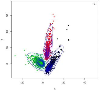
Figure 2. A simulated dataset from a three-component skewtmixture

the supplementary information of [8]. Method 2 attempts to obtain the exact values at each stage of the iterative process, where the terme(₄k_,ij) is calculated by truncating an infinite series expansion of it. With Method 3, the default pre-defined values for the degrees of freedom νi= 4 (i= 1, . . . , g)are

adopted. A simulation study has been conducted to compare the three methods.

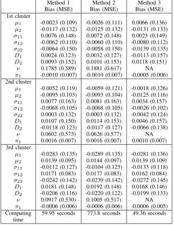
We generate 100 datasets from a three-component skew t mixture model. For each dataset, there are 1000 two-dimensional samples, in which 300 samples come from the first component, 300 from the second, and 400 from the third. One example dataset is plotted in Fig. 2. With this simulation study, true parameter values are used as the initial values. The EM algorithm proceeds until the relative change of log likelihood is less than 0.0001, or until it reaches the maximum number of iterations 100, whichever first occurs. The total computing time, the bias, and mean square errors (MSEs) for each method are summarised in Table I.

From Table I, it can be observed that Method 2 takes the longest computing time (more than twelve times of Method 1 and fifteen times of Method 3). Both Methods 1 and 2 overestimate the degrees of freedom νi, and are unbiased in

the estimation ofθi (i= 1,2,3). V. ANEXAMPLE

A flurescence-activated cell sorting (FACS) dataset is used as an illustration. Flurescence-activated cell sorting machines yield readout on large mixed populations of single cells, with aroundn= 5,000−50,000cells from blood sam-ples of individuals with multiple sclerosis and other diseases. The flurescence intensities of tagged antibodies are measured

562

447 484

(5)

Table I

COMPARISON OFTHREEMETHODS FORESTIMATING THEDEGREES OF FREEDOM

Method 1 Method 2 Method 3 Bias (MSE) Bias (MSE) Bias (MSE) 1st cluster μ1 -0.0023 (0.109) -0.0026 (0.111) 0.0066 (0.136) μ2 -0.0117 (0.132) -0.0125 (0.132) -0.0131 (0.133) σ11 0.0076 (0.148) 0.0072 (0.148) 0.0023 (0.149) σ12 -0.0062 (0.110) -0.0060 (0.110) -0.0080 (0.112) σ22 -0.0064 (0.150) -0.0058 (0.150) -0.0139 (0.135) D1 0.0024 (0.123) 0.0032 (0.127) -0.0113 (0.157) D2 0.0093 (0.152) 0.0101 (0.153) 0.0118 (0.151) ν 0.1785 (0.589) 0.1881 (0.617) NA π1 -0.0010 (0.007) -0.0010 (0.007) -0.0005 (0.006) 2nd cluster μ1 -0.0052 (0.119) -0.0059 (0.121) -0.0018 (0.126) μ2 -0.0095 (0.103) -0.0093 (0.104) -0.0125 (0.116) σ11 0.0077 (0.163) 0.0081 (0.163) 0.0034 (0.157) σ12 -0.0068 (0.105) -0.0068 (0.105) -0.0026 (0.102) σ22 0.0003 (0.132) 0.0003 (0.132) -0.0042 (0.124) D1 0.0107 (0.150) 0.0114 (0.153) 0.0046 (0.157) D2 -0.0118 (0.123) -0.0117 (0.127) -0.0066 (0.138) ν 0.0602 (0.573) 0.0626 (0.577) NA π1 0.0016 (0.007) 0.0016 (0.007) 0.0010 (0.007) 3rd cluster μ1 -0.0283 (0.135) -0.0289 (0.135) -0.0281 (0.136) μ2 0.0139 (0.095) 0.0144 (0.097) 0.0139 (0.109) σ11 -0.0112 (0.127) -0.0104 (0.125) -0.0133 (0.118) σ12 0.0171 (0.083) 0.0177 (0.083) 0.0162 (0.084) σ22 -0.0242 (0.142) -0.0239 (0.142) -0.0272 (0.145) D1 0.0181 (0.148) 0.0192 (0.148) 0.0168 (0.146) D2 -0.0206 (0.116) -0.0220 (0.122) -0.0199 (0.133) ν 0.0917 (0.530) 0.1005 (0.517) NA π1 -0.0006 (0.006) -0.0006 (0.006) -0.0006 (0.005) Computing 59.95 seconds 773.8 seconds 49.36 seconds

time

by the scanners and are reported as multi-dimensional points (in general 4 or 8 colour FACS corresponding to different markers). The objective here is to cluster the blood cells on the basis of multivariate FACS data with an attempt to detect important subpopulations of regulatory cells. However, the FACS data are also multimodal, asymmetric, and have many outliers. Thus, the fitting of multivariate normal or t mix-ture models for the analysis of FACS data often generates distorted contours and may lead to invalid conclusions.

The dataset was captured using a BD Biosciences FACS Calibur system [16]. It consists of n = 4952 blood cells samples stained for 4 markers (CD4, CD56, CD8, and CD3). The proposed multivariate skewtmixture model is fitted to the 4-dimensional data with g = 2 tog = 15 components. Based on the Bayesian information criterion (BIC) for model selection [1], [17], we identify there are eight clusters of blood cells. The pairwise two-dimensional contours of the fitted skew t mixture model are presented in Fig. 3. The contour lines indicate the asymmetric nature of the FACS data, such as the cluster indicated by blue coloured dots in the graph CD56 against CD4, and the cluster indicated by black coloured dots in the graph CD8 against CD56. In addition, it can be seen from Fig. 3 that the model fits well

0.0 1.0 2.0 0.0 0.5 1.0 1.5 2.0 2.5 3.0 CD4 CD56 0.0 1.0 2.0 01234 CD4 CD8 0.0 1.0 2.0 01234 CD4 CD3 0.0 1.0 2.0 3.0 01234 CD56 CD8 0.0 1.0 2.0 3.0 01234 CD56 CD3 0 1 2 3 4 01234 CD8 CD3

Figure 3. Two-dimensional contours of the fitted skewtmixture model

to the data. The clusters so formed and their estimated model parameters may be used to infer various disease signatures in FACS samples and match corresponding cell populations across samples that enables quantitative downstream analy-sis, such as classification and prediction of clinically relevant phenotypes [8].

VI. DISCUSSION

We have developed mixtures of multivariate skew t dis-tributions to handle highly asymmetric multivariate data. A singularity handling procedure has been considered to solve singularity problems within the framework of the EM algorithm. We also compare three methods for estimating the degrees of freedom for the component-t distributions. The proposed method has been applied to a real flurorescence-activated cell sorting dataset.

An alternative method has been considered recently to handle asymmetric data [18]. Their method transforms the asymmetric data via a Box-Cox transformation to minimize skewness of the data. Symmetric t distributions are then adopted to model the transformed data. In contrast, our pro-posed multivariate skewtmixture approach models directly the asymmetric populations and hence gets to understand the distinctive shape and location of each sub-population. These estimated parameters may further be employed to identify distinctive features that are relevant to predict disease out-comes.

Multivariate skew t mixture modelling can be readily applied to other important pattern recognition problems. For

563

448 485

(6)

example, it can offer insights into FACS experiment design by detecting redundant (i.e. less informative) and discrimi-native (i.e. more informative) antibody profiles. Applications of the model can be found in wide areas of scientific fields where (multivariate) data exhibit a mixture of asymmetric patterns with atypical observations; see, for example, [9], [10], [11].

With applications of mixture models, the likelihood equa-tion will have multiple roots corresponding to local maxima. The EM algorithm described in Section II.B should be applied from a wide choice of initial values in any search for all local maxima [6]. The intent is to choose as the maximum likelihood estimate of the parameter vectorΨthe local maximizer corresponding to the largest of the local maxima located [1]. In practice, consideration has to be given to the problem of relatively large local maxima that occur as a consequence of a fitted component having a very small (but nonzero) generalized variance (the determinant of the covariance matrix). Such a component corresponds to a cluster containing a few data points either relatively close together or almost lying in a lower-dimensional subspace. As described in Section III, a singularity handling procedure is required to identify the spurious local maximizers [1].

ACKNOWLEDGMENT

The work was supported by grants from the Australian Research Council and the University of Queensland, Aus-tralia.

REFERENCES

[1] G. J. McLachlan and D. Peel, Finite Mixture Models. New York: Wiley, 2000.

[2] S. K. Ng and G. J. McLachlan, “Speeding up the EM algorithm for mixture model-based segmentation of magnetic resonance images,”Pattern Recognition, vol. 37, pp. 1573–1589, 2004. [3] S. K. Ng, G. J. McLachlan, K. Wang, L. Ben-Tovim Jones, and

S. W. Ng, “A mixture model with random-effects components for clustering correlated gene-expression profiles,”

Bioinfor-matics, vol. 22, pp. 1745–1752, 2006.

[4] K. Wang, K. K. W. Yau, and A. H. Lee, “A hierarchical Poisson mixture regression model to analyse maternity length of hospital stay,”Stat. Med., vol. 21, pp. 3639–3654, 2002. [5] A. P. Dempster, N. M. Laird, and D. B. Rubin, “Maximum

likelihood from incomplete data via the EM algorithm (with discussion),”J. Roy. Stat. Soc. B, vol. 39, pp. 1–38, 1977. [6] G. J. McLachlan and T. Krishnan, The EM Algorithm and

Extensions, 2nd ed. New Jersey: Wiley, 2008.

[7] G. J. McLachlan and D. Peel, “Robust cluster analysis via mixtures of multivariatet-distributions,”Lect. Notes Computer

Science, vol. 1451, pp. 658–666, 1998.

[8] S. Pyne, X. Hu, K. Wang, E. Rossin, T.-I. Lin, L. M. Maier, C. Baecher-Allan, G. J. McLachlan, P. Tamayo, D. A. Hafler, P. L. De Jager, and J. P. Mesirov, “Automated high-dimensional flow cytometric data analysis,”Proc. National Acad. Sciences USA, vol. 106, pp. 8519–8524, 2009.

[9] A. Azzalini and A. Capitanio, “Statistical applications of the multivariate skew-normal distribution,” J. Roy. Stat. Soc. B, vol. 61, pp. 579–602, 1999.

[10] A. Azzalini and A. Capitanio, “Distributions generated by perturbation of symmetry with emphasis on a multivariate skew t-distribution,”J. Roy. Stat. Soc. B, vol. 65, pp. 367–389, 2003. [11] A. Azzalini and A. Dalla Valle, “The multivariate skew-normal distribution,”Biometrika, vol. 83, pp. 715–726, 1996. [12] A. K. Gupta, “Multivariate skew t-distribution,” Statistics,

vol. 37, pp. 359–363, 2003.

[13] T. I. Lin, J. C. Lee, and W. Hsieh, “Robust mixture modeling using the skewtdistribution,”Stat. Comp., vol. 17, pp. 81–92, 2007.

[14] T. I. Lin, J. C. Lee, and S. Y. Yen, “Finite mixture modeling using the skew normal distribution,”Stat. Sinica, vol. 17, pp. 909–927, 2007.

[15] S. K. Sahu, D. K. Dey, and M. D. Branco, “A new class of multivariate skew distributions with applications to Bayesian regression models,”Canadian J. Stat., vol. 31, pp. 129–150, 2003.

[16] L. M. Maier, D. E. Anderson, P. L. De Jager, L. S. Wicker, D. A. Hafler, “Allelic variant in CTLA4 alters T cell phospho-rylation patterns,” Proc. National Acad. Sciences USA, vol. 104, pp. 18607–18612, 2007.

[17] G. Schwarz, “Estimating the dimension of a model,” Ann.

Stat., vol. 6, pp. 461–464, 1978.

[18] K. Lo, R. R. Brinkman, and R. Gottardo, “Automated gating of flow cytometry data via robust model-based clustering,”

Cytometry A, vol. 73, pp. 321–332, 2008.

564

449 486