Bayesian Analysis of Markov Switching Vector Error Correction Model

Title

Bayesian Analysis of Markov Switching Vector Error

Correction Model

Author(s)

Sugita, Katsuhiro

Citation

Issue Date

2006-11

Type

Technical Report

Text Version

URL

http://hdl.handle.net/10086/16990

#2006-13

Discussion Paper #2006-13

Bayesian Analysis of Markov Switching

Vector Error Correction Model

by

Bayesian Analysis of Markov Switching Vector Error

Correction Model

Katsuhiro Sugita∗

Graduate School of Economics, Hitotsubashi University, 2-1, Naka,

Kunitachi, Tokyo, 186-8601, Japan

E-Mail: [email protected]

Abstract

This paper introduces a Bayesian approach to a Markov switching vector error correction model that allows for regime shifts in the intercept terms, the lag terms, the adjustment terms and the variance-covariance matrix. The pro-posed Bayesian method allows for estimation of the cointegrating vector within a nonlinear framework through Gibbs sampling so that it generates more effi-cient estimation than classical approaches that require a multi-stage maximum likelihood procedure. The Bayes factors are applied to test for Markov switching and model specifications. We apply the proposed model to U.S. term structure of interest rates allowing the risk premium and other parameters in the model to change with regime.

Key words: Bayesian inference; Nonlinear cointegration; Markov switching model;

Gibbs sampling; Bayes factor;

∗_{The author would like to thank Mike Clements and the participants of seminar at Warwick for their}

1

Introduction

This paper proposes a Markov switching vector error correction model (MS-VECM) that allows for regime shifts in the intercept terms, the lag terms, the adjustment terms and the variance-covariance matrix in a vector error correction model, using a Bayesian approach with a Markov chain Monte Carlo method.

A number of studies consider nonlinear cointegration models with regime switch-ing. Balke and Fomby (1997) consider a threshold cointegration model in order to investigate the model in which there is discontinuous adjustment to a long-run equilib-rium, based on the idea that only when the deviation from the equilibrium exceeds a critical threshold, do the benefits of adjustment exceed the costs and, hence economic agents act to move the system back toward the equilibrium. Other research using threshold cointegration model include Anderson (1997), Tsay (1998), Martens et al (1998), and Clements and Galvao (2002). Instead of threshold cointegration model, nonlinear cointegration model using Hamilton’s (1989) Markov regime switching pro-cess is also developed (Krolzig, 1997). Hall et al (1997) analyze the permanent income hypothesis using a single equation cointegration model with Markov regime switching. Psaradakis et al (2004) employ Markov switching to analyze an error correction model in a single equation. A vector error correction model with Markov regime switching is applied by Sarno and Valente (2005) for forecasting stock returns, and by Clarida et al (2006), who show regime switching in the term structure of interest rates.

Estimation for a MS-VECM by classical methods requires a multi-stage maximum likelihood procedure. The first stage consists of testing for the number of cointegrating relationships in the system and estimating the cointegrating vectors by implementing Johansen’s (1988, 1991) maximum likelihood method. Then, the second stage consists of estimating other parameters in the model by maximum likelihood method. Thus, the cointegrating vectors and other parameters in a nonlinear vector error correction model are estimated assuming the model is linear. The final stage consists of the im-plementation of an expectation-maximization (EM) algorithm for maximum likelihood

estimation for unobserved Markov state variables conditional on estimated values of the cointegrating vectors and other parameters by maximum likelihood. Thus, to es-timate the Markov state variables, the maximum likelihood eses-timates are treated as if they were the true values.

By applying a Bayesian approach, estimation of the MS-VECM is more efficient as inference on the state variable is based on a joint distribution, rather than a conditional distribution. The cointegrating vectors are estimated based on a joint distribution of other variables including the state variables, so that it allows estimation of the cointe-grating vectors within a nonlinear framework, rather than assuming that the model is linear.

This paper proposes a Bayesian approach to a MS-VECM that allows the intercept, the lag terms, the adjustment coefficients, and the variance-covariance matrix to shift with Markov process. For a Bayesian approach to a MS-VECM, Paap and van Dijk (2003) propose a nonlinear VECM where the intercept terms are affected by Markov regime shift in order to investigate U.S. consumption and income. They employ a Bayesian cointegration analysis based on Kleibergen and Paap (2002) and Kleibergen and van Dijk (1998), which requires linear normalizing restrictions on the cointegrat-ing vectors, that are criticized by Strachan (2003) as becointegrat-ing likely to be invalid. Stra-chan and van Dijk (2003a) and StraStra-chan and Inder (2004) discuss the further problems associated with the use of linear normalizing restrictions, and propose the Grassman approach that places a valid prior on the cointegrating space. See Koop et al (2006b) for details. In this paper, to estimate the cointegrating vectors, we apply Strachan and Inder’s (2004) Bayesian method, that elicits a valid prior for the cointegrating space.

Our model in this paper is more general than Paap and van Dijk (2003), and is flexible to modify in order to consider the model in which other parameters are also subject to the regime shift. For example, in this paper we assume that the cointegrating vectors are unaffected by the regime shifts. It is, however, possible to consider the model where the cointegrating vectors are also dependent on the regime shifts. Also, it is possible to consider the constant in the cointegrating vectors to be affected by the

regime shifts by a slight modification. We present this modification in the application of the model which consider the regime dependent risk premium term to investigate U.S. term structure of interest rates.

The plan of the paper is as follows. Section 2 presents estimation method for the MS-VECM using a Gibbs sampler. We specify prior densities and likelihood func-tions, and then derive the posterior distributions. In Section 3, we describe testing for Markov switching and the number of cointegrating rank as model selection by Bayes factors. For testing for nonlinearity, the Schwarz BIC is used to approximate the Bayes factors. To determine the number of rank, the Savage-Dickey density ratio is applied to compute the Bayes factors. Then we show simulated experiments with artificially generated data to evaluate the performance of detecting an appropriate model by the proposed method. Section 4 illustrates application to U.S. term structure of interest rates, using the MS-VECM where the risk premium term is also affected by the regime shifts as well as the intercept terms, the lag terms, the variance-covariance matrix, and the adjustment coefficients. Section 5 contains concluding remarks. The computa-tions reported in this paper were performed using code written in the Ox programming language (Doornik, 1998).

2

Markov Switching Vector Error Correction Model

This section introduces a MS-VECM and presents a Bayesian approach to estimate this model. Let Xt denote an I(1) vector of n-dimensional time series with r linear coin-tegrating relations. A VAR(p) system with normally distributed Gaussian innovations ε∼iidN(0,Σ)can be written as a vector error correction model (VECM)

∆Xt =µ+αβ0Xt−1+

p−1

∑

i=1

Ψi∆Xt−i+εt (1)

whereα(n×r)is adjustment term; andβ0(n×r)is cointegrating vector. If we assume that the intercept term µ, the adjustment termα, the lag terms Ψi, and the variance-covariance matrixΣin the VECM are subject to an unobservable discrete state variable

st=i where i=1,2, . . . ,m, then the VECM representation is written as ∆Xt=µ(st) +α(st)β0Xt−1+ p−1

∑

i=1 Ψi(st)∆Xt−i+εt (2)

whereεt are assumed N(0,Σ(st))and independent over time. Dimensions of matri-ces are µ and ε (n×1), Ψi andσ (n×n). The state variable st evolves according to a m-state, first-order Markov switching process with the transition probabilities, p(st =i|st−1= j) =pi j, i,j=1, . . . ,m.

Equation (2) can be rewritten in the matrix format as

Y =W B+E (3) where Y= (∆Xp, . . . ,∆XT)0, W= (I1Zβ, . . . ,ImZβ), B= (α,Γ0)0, Z= (Xp−1, . . . ,XT−1)0, E= (εp, . . .εT)0,α= (α1, . . . ,αm), Γ= (µ1, . . . ,µm,Ψ1,1, . . . ,Ψp−1,1, . . . ,Ψm,1, . . . ,Ψm,p−1)0, X=       s1,p · · · sm,p s1,p∆X_p0−1 · · · s1,p∆X 0 1 · · · sm,p∆X 0 p−1 · · · sm,p∆X 0 p−1 .. . . .. ... ... . .. ... ... ... . .. ... s1,T · · · sm,T s1,T∆XT0−1 · · · s1,T∆0T−p+1 · · · sm,T∆XT0−1 · · · sm,T∆XT0−p+1       .

Letτbe the number of rows of Y , so thatτ=T−p+1, then X isτ×m(1+n(p−1)), Γis m(1+n(p−1))×n, W isτ×κwhereκ=m(1+n(p−1) +r), and B isκ×n. si,j in X is an indicate variable such that it equals to 1 if regime is i and 0 otherwise.

I

i in W is an indicator matrix(τ×τ) where the diagonal elements are 1 if tth regime is i, otherwise 0, and the off-diagonal elements are all 0. Equation (3) represents the stacked form of (2).

2.1 Prior Distributions and Likelihood Functions

In selecting a prior density for cointegrating vectors, one approach is to choose an informative prior such as a normal or a Student t distribution with r2linear normaliza-tion restricnormaliza-tions onβfor identification such thatβ0= (Ir,β0?) whereβ? is(n−r)×r

choose this type of prior with linear normalization onβ. This prior with linear nor-malization, however, is criticized by Strachan (2003) and Strachan and Inder (2004) as invalid because this normalization restricts the estimable region of the cointegrating space. Instead of using this prior, they propose the Grassman approach that places a prior on the cointegrating space rather than the cointegrating vectors. There is a num-ber of research based on the Grassman approach. Strachan and van Dijk (2003a), for example, analyze a vector error correction model using an uniform prior for the coin-tegrating space. Strachan and van Dijk (2003b) investigate an issue of model selection with a proper diffuse prior on the cointegrating vector. Koop et al (2006a) extend to a panel cointegration model, based on the Grassman prior. Koop et al. (2006b) discuss the prior elicitation for the cointegrating vector in detail. In this paper, we also adopt the Grassman approach to place a noninformative prior on the cointegrating space as

g(β)∝ π−(n−r)r r

∏

j=1 Γ[(n+1−j)/2] Γ[(r+1−j)/2] (4) whereΓ[q] =R∞ 0 uq

−1_e−u_{du, q>0 with identification restrictions,β}0_{β=In, that do not}

distort the weight on the cointegrating space.

For a prior for the transition probabilities pi j, i,j=1, . . . ,m, we assign a beta distribution, assuming m=2

p00∼beta(u00,u01) (5)

p11∼beta(u11,u10) (6)

where beta refers to a beta distribution with densityπ(pii|uii,ui j) =_ΓΓ₍(_uiiuii₎+_Γ(ui j_{ui j})₎puii_ii−1(1−

pii)ui j−1.

With regard to priors for B, Ωi, we assume prior independence between B and Ωi such that p(B,Ω1, . . . ,Ωm) =p(B)∏mi=1p(Ωi). We assign prior for the variance-covariance matrix as an inverted Wishart distribution with the degrees of freedom h

as

Ωi∼IW(Φi,hi) (7)

whereΦi∈Rn×n. As for a prior for B, we consider the vector form of B and assign a

multivariate normal as

vec(B)∼MN(vec(B0),ΣB) (8) where MN refers to a multivariate normal with mean vec(B0)∈Rκn×1, k=m(1+

n(p−1) +r) and variance-covariance matrix ΣB ∈Rκn×κn. We assume thatαi, i= 1, . . . ,m, is distributed independently, so thatΣBis defined as

ΣB=    Σα 0 0 ΣΓ    (9)

whereΣ_αis nrm×nrm matrix such thatΣ_α=V_α⊗Irm, V_α(n×n)is prior variance-covariance matrix of αi ∼MV N(α,V_α); ΣΓ is n(m+n(p−1))×n(m+n(p−1)) matrix and is prior variance-covariance matrix of Γ|α∼MV N(Γ,Σ_Γ). This inde-pendence relation of distributions amongα1, . . . ,αmis convenient for determining the cointegrating rank using the Savage-Dickey density ratio described in Section 3.

The likelihood function for B,Ω1, . . .Ωm,βand the state variablesSTe ={s₁,s₂, . . . ,sT}0 is given by, LB,β,Ω1, . . . ,Ωm,Se_T |Y ∝

∏

m i=1 |Ω_i|−ti/2 ! exp −1 2tr " m

∑

i=1 Ω−1 i (Yi−WiB)0(Yi−WiB) #! (10) = m

∏

i=1 |Ω_i|−ti/2 ! exp −1 2 m

∑

i=1 h (vec(Yi−WiB))0(Ωi⊗Iτ)−1(vec(Yi−WiB)) i ! (11)

where Yi=

_I

iY , Wi=

_I

iW and ti is the total number of observations when st =i, i= 1,2, . . . ,m.

The likelihood function for the transition probabilities pi j, i,j=1,2, . . . ,m, which are independent of the data but conditional on the set of the state variables, is given assuming m=2: L p11,p22|STe =pm11 11 (1−p11) m12_pm22 22 (1−p22) m21 ₍₁₂₎

where mi,j, i,j = 1 or 2, denotes the number of the transition from the regime i to j, that can be counted from givenSe_T.

2.2 Posterior Specifications

In this subsection we derive the posterior densities from the priors and the likelihood functions. First, we derive the state variableSeτ={s₁,s₂, . . . ,sτ}0 by the multi-move Gibbs sampler, then derive the posterior distributions for other parameters.

To sample the state variableSeτwe employ the multi-move Gibbs sampling method, which is originally proposed by Carter and Kohn (1994) and is applied to a Markov switching model by Kim and Nelson (1998). The multi-move Gibbs sampling refers to simulating st, t=1,2, . . . ,T , as a block from the following conditional distribution:

p e S_τ|Θ,Y =p(s_τ|Θ,Y) τ−1

∏

t=p p(s_τ|s_τ+1,Θ,Y) (13)

whereΘ={B,β,Ω1,Ω2,p11,p22}. The first term of the right hand side of the above

equation, p(sτ|Θ,Y), can be obtained from running the Hamilton filter (Hamilton, 1989). To draw stconditional on st+1,Θand Y , we use the following results:

p(st |st+1,Θ,Y) =

p(st+1|st,Θ,Y)p(st |Θ,Y)

p(st+1|Θ,Y)

∝p(st+1|st)p(st |Θ,Y) (14)

the Hamilton filter. Using Equation (14) we compute: Pr(st=0|st+1,Θ,Y) = p(st+1|st=1)p(st =1|Θ,Y) ∑1 j=0p(st+1|st= j)p(st= j|Θ,Y) (15)

Once above probability is computed, we draw a random number from a uniform distri-bution between 0 and 1, and if the generated number is less than or equal to the value calculated by (15), we set st =1, otherwise, set equal to 0.

After drawingSeτby multi-move Gibbs sampling, we generate the transition prob-abilities, p11and p22, by multiplying (5) and (6) by the likelihood function (12)

p p11,p22|Seτ ∝pu22+m22−1 22 (1−p22) u21+m21−1_pu11+m11−1 11 1−pu12+m12−1 11 (16)

Next, we can construct X and Z in (3) using the draw of Seτ, and then the joint posterior distribution can be obtained from the priors given in (7) and (8) and the likelihood function for B,β,Ωi,andSeτ, that is,

pB,β,Ω1, . . . ,Ωm,Seτ|Y ∝pB,β,Ω1, . . . ,Ωm,Se_T LB,β,Ω1, . . . ,Ωm,Se_T|Y ∝ g(β) " m

∏

i=1 |Ji|hi/2|Ωi|−(ti−1)/2 # exp ( −1 2 " tr m

∑

i=1 Ω−1 i ! + m

∑

i=1 h

vec(Yi−WiB)0(Ωi⊗Iτ)−1vec(Yi−WiB) i

+vec(B−B0)0Σ−B1vec(B−B0)

#)

(17)

where g(β) refers to the prior forβ given in (4). From the joint posterior (17), we have the following posterior distributions (see Appendix A.1 for derivation of these posteriors): Ωi|β,B,Seτ,Y ∼IW (Y_i−W_iB) 0 (Yi−WiB) +Φi,ti+hi (18)

vec(B)|Ω_i,β,Seτ,Y ∼N(vec(B_?),M_?) (19) where M?= ( Σ−1 B + m

∑

i=1 Ω−1 i ⊗ W 0 iWi )−1 vec(B?) =M? ( Σ−1 B vec(B0) + m

∑

i=1 h (Ωi⊗Iκ)−1vec Wi0Yi i )

For the posterior for β, according to Strachan and Inder (2004), let z1,t be the (t−1)th_{row of Z and z}

2,t be the tthrow of X , then p(β|Seτ,Y)∝g(β) β0D₀β −τ/2 β0D₁β (τ−n)/2 (20) where D0=D1−D2, D1=S11and D2=S10S₀₀−1S01, Sjk=Mjk−Mj2M₂₂−1M2k, Mjk= hjk+∑z0j,tzk,t, hjk=0 if j6=k, hj j=ϕI.

The posterior distributions forΩiin (18), B in (19), andβin (20) are not convenient analytical forms. Rather they are conditional on other parameters which must be esti-mated. Gibbs sampler can be employed to generate random draws from the conditional posteriors. While the conditional posterior densities forΣiand B are known form, the posterior forβ in (20) is not a standard form and thus can be drawn by employing importance sampling, the Metropolis-Hastings algorithm (see Chib and Greenberg, 1995) or the Griddy-Gibbs sampling (see Ritter and Tanner, 1992). In this paper, we choose the Griddy-Gibbs sampling technique because the algorithm does not require the specification of function that approximate the distribution. Choosing the Griddy-Gibbs sampler, however, requires the appropriate choice of the grid of points and the computing cost is much higher than other algorithms. The algorithm is provided in Appendix A.2 for convenience.

to generate sample draws. The following steps can be replicated until convergence is achieved.

• Step 1: Set j=1. Specify starting values for the parameters in the model, p(_ik0), B(0),β(0)andΩ(_i0). • Step 2: GenerateSe (j) τ = n s₁(j),s₂(j), . . . ,s(_τj) o0 from p e Sτ|Θ(j−1)_{,Y, where}Θ₌

{B,Ω1, . . . ,Ωm,β,pik}in (13), using multi-move Gibbs sampling algorithm.

• Step 3: Generate the transition probabilities(pik)(j)from p pik|Se (j) τ in (16).

• Step 4: Generateβ(j)from p(β|Se

(j)

τ ,Y)in (20) using the Griddy-Gibbs sampling algorithm.

• Step 5: Generate B(j)from p(vec(B)|β(j)_,Ω(j−1)

i ,Se

(j)

τ ,Y)in (19).

• Step 6: GenerateΩ(_ij)from p(Ωi|β(j),B(j),Se

(j)

τ ,Y)in (18).

• Step 7: Set j=j+1, and go to Step 2.

Step 2 through Step 7 can be iterated N times to obtain the posterior means or standard deviations. Note that the first N0times iterations are discarded in order to attenuate the

effect of the initial values.

3

Testing for Markov Switching, Cointegrating Rank, and

Model Selection by Bayes Factors

In this paper, testing for Markov switching and the cointegrating rank is treated as a problem of model selection. In Bayesian framework, the posterior model probability p(

M

j |Y) is used to assess the degree of support for each model,

M

j. From the Bayes rule, we have p(

M

j|Y) =p(Y |

M

j)p(

M

j)/p(Y), where p(Y |

M

j)is referred to as the marginal likelihood for

M

j; and p(

M

j) is the prior model probability for

M

j. Since p(Y) is often hard to calculate, comparison of two models, j and i, by the posterior odds ratio, POji, is often used to obtain the posterior model probability.

The posterior odds ratio is defined as the ratio of their posterior model probabilities as POji=p(

M

j|Y)/p(

M

i|Y) = p(Y

|Mj)p(Mj)

p(Y|_Mi)p(Mi), where the ratio of the marginal likelihoods p(Y|Mj)

p(Y|Mi) is defined as the Bayes factor. With the posterior odds ratios, we can obtain the posterior model probability as p(

M

j|Y) =POji/∑Mk=1POkiwhere M is the number of models under consideration. Thus, in order to obtain the posterior model probability by the posterior odds, we need to calculate the Bayes factor.

There are several methods to calculate the Bayes factor such as Chib (1995), Gelfand and Dey (1994), the Savage-Dickey density ratio (see Verdinelli and Wasser-man, 1995), and the Schwarz Bayesian information criterion (BIC) approximation method (Schwarz, 1978). Among these, we choose the Schwarz BIC method to test for nonlinearity and select the most appropriate model since other methods are not possi-ble or difficult to perform.1 The Schwarz BIC can give a rough approximation to the Bayes factors. It is, however, easy to implement and does not require evaluation of the prior distribution, as Kass and Raftery (1995) note. The Schwarz BIC to approximate the Bayes factors is employed by Wang and Zivot (2000) for detecting the number of structural breaks. The Schwarz BIC for

M

jis calculated as

BICj=−2 lnL b θj|Y ;

M

j +qjln(t) (21) whereLθb_j|Y ;

M

_j

denotes the likelihood function under the model j; qjdenotes the total number of estimated parameters in

M

j. The likelihood functionL

b

θj|Y ;

M

j

is evaluated atθbj, the posterior means of the parameters for

M

j.

With the Schwarz BICs for

M

jand

M

i, the Bayes factor for

M

jagainst

M

ican be approximated by

BFji=exp[−0.5(BICi−BICj)]. (22)

1 _{For example, a method by Chib (1995) requires to know the full form of prior, likelihood, and}

posterior. In the MS-VECM, the full forms of posterior forβin (20) is difficult to obtain. In this case, Chib and Jeliazkov (2001) show how the marginal likelihood can be calculated using the output from the Metropolis-Hastings algorithm.

The Savage-Dickey density ratio method is applicable only to nested models, while the Gelfand and Dey method is not suitable to multivariate models.

With the prior odds, defined as p(

_M

j)/p(

M

i), the posterior odds can be computed by multiplying the Bayes factor by the prior odds as PosteriorOddsji=BFji×PriorOddsji. By using the Schwarz BIC to approximate to logarithm of the Bayes factor, it is easy to test Markov switching cointegration as a problem of model selection. In our case, we compute the Schwarz BIC such that

BICj = -2 lnL B,Σ1, . . . ,Σm,β,Seτ,pik|Y ;

M

_j +qjln(t) = −2 n lnL B,Σ1, . . . ,Σm,β,Seτ|Y ;

M

_j +lnL pik|Seτ;

M

_j o +qjln(t)

To determine the number of cointegrating rank, Strachan and Inder (2004) employ the Laplace approximation method to calculate the Bayes factors. In this paper, instead of applying the Laplace approximation method, we choose the Savage-Dickey density ratio to calculate the Bayes factors to determine the number of cointegrating rank. The Bayes factor comparing zero rank r=0 and non-zero rank r=r∗is obtained using the Savage-Dickey density ratio as follows:

BF(r=0|r=r∗) = BF(α=0|α6=0) = p(α=0|Y,

M

r∗)

p(α=0|

_M

r∗) (23)

where r∗>0 is the number of rank to test;

M

r∗ denotes a model with rank r∗; the

denominator is the prior density evaluated atα=0; and the numerator is the posterior density evaluated atα=0. The prior for B, vec(B)∼MN(vec(B0),ΣB)withΣBdefined in (9), implies p(α) =∏m_i=+₁1p(αi), whereαi∼MV N(α,V_α). The posterior forαi is also independently distributed asαi |β,Ωi,Yi∼MV N(αi,Vα,i) where Vα,i = (V−_α1+ Z_i0ZiΩ−i 1)−1andαi=Vα,i(V−_α1α+Zi0(Yi−XiΓi)Ωi). Since 1 N−N0 N

∑

j=N0+1 p(α=0|β(j),Ω(j),Y,r∗)→p(α=0|Y,

M

r∗) (24)

To evaluate the performance of detecting the Markov switching nonlinearity by the Schwarz BIC, we conducted Monte Carlo simulations. We consider three-variable MS-VECM for the experiments. The data generating processes (DGPs) are given as the following:

M

1 : ∆Xt =µ0+α0β0Xt−1+Ψ0∆Xt−1+σ0εt

M

2 : ∆Xt =µ(st) +α(st)β0Xt−1+Ψ(st)∆Xt−1+σ0εt

M

3 : ∆Xt =µ0+α(st)β0Xt−1+Ψ0∆Xt−1+σ(st)εt

M

4 : ∆Xt =µ(st) +α(st)β0Xt−1+Ψ(st)∆Xt−1+σ(st)εt where µ(st =0) =µ0=(0.2, 0.2, 0.2)’, µ(st =1) =µ1=(-0.2, -0.2, -0.2)’, α(st =0) = α0=(-0.2, -0.2, 0.2)’,α(st=1) =α1=(0, 0, 0)’,β0=(1, -1, 1),εt∼NID(0, I3),σ(st= 0) =σ0=0.5I3,σ(st =1) =σ1=0.1I3,Ψ(st =0) =Ψ0=0.5I3, andΨ(st =1) =

Ψ1=0.2I3the sample size T ={100, 200, 500}. The transition probabilities are given

as (p00, p11)=(0.95, 0.95). These four DGPs represent:

M

1: Linear VECM model.

M

2: Homoskedastic MS-VECM with regime dependent mean

M

3: Heteroskedastic MS-VECM with constant mean

M

4: Heteroskedastic MS-VECM with regime dependent mean

It might be possible to compute Bayes factors for all model

M

1 -

M

4 to select the most appropriate model. However, if the true model is linear as

M

1, computation of the Bayes factors for

M

2 -

M

4 might not be feasible because of the problem that the state variables and the transition probabilities are not identified through the Gibbs sampling, causing a convergence problem in the Gibbs sampler. Kim and Nelson (2001) overcome this problem by employing ’pseudo priors’ (see Carlin and Chib, 1995). In this paper we restrict a priori that a certain percentage of the observations lies in each regime as Koop and Potter (1999) in order to avoid the problem. When the total number of either regime occurred in the generated state variables at j-th iteration

of Gibbs sampling, that is,∑τ_i=1s(_ij)or∑τ_i=1(1−s(_ij)), is less than given value, say, 5 percent of the sample size, then the previously drawn set of state variables,Se

(j−1)

τ , is used in the j-th iteration of the Gibbs sampler by settingSe

(j)

τ =Se

(j−1)

τ .

The Bayes factors were computed for all models (

_M

1 -

_M

4) to calculate the pos-terior model probability for each model. For prior hyperparameters, we setΦi=0.01I3

and hi=0.001 for all i in (7),ΣB=100Iκn and B0=0 in (8) favoring the absence of

cointegration. These values are assigned to ensure fairly large variances for represent-ing prior ignorance. For prior hyperparameters for the transition probabilities, we set u00=u11=9, u01=u10=1 in (5) and (6). The number of cointegration rank and the

lag length are assumed to be known. Each simulation is replicated 1000 times. For each replication of the simulations, the Griddy-Gibbs sampler is employed with 5,000 draws with the first 500 discarded to generate the cointegrating vector with the interval of integration (the deterministic Simpson’s rule is used) for each element ofβfrom -6.00 to 6.00 with the number of the grid at 1200 to avoid significant truncation of the posterior density.

Table 1 summarizes the results of Monte Carlo simulations for model selection. The value in each element of the Table represents the average posterior model prob-ability. When the true model is the linear VECM,

M

1, the average posterior model probability selects the correct model

M

1 with more than 90% even when T =100. When the true model is the MS-VECM,

M

2,

M

3 or

M

4, the average posterior model probability selects the correct model with less than 90% for the three DGPs when T =100. Increasing the sample size to 200 improves the performances as the correct model is selected with more than 90%.

4

Application: U.S. Term Structure of Interest Rates

We present an empirical study using the MS-VECM to analyze U.S. term structure of interest rates. It is possible to apply the MS-VECM of the form (2) to examine the expectations hypothesis of U.S. term structure of interest rates. However, with some

minor modifications, the model can be extended to allow the risk premium term in the cointegrating vector to shift with regime, rather than assuming that the risk premium is constant. With this model, we can investigate nonlinearity of U.S. term structure of interest rates by changes in monetary policy.

4.1 Expectation Hypothesis

The expectations hypothesis of the term structure of interest rates implies an f -period interest rate is the weighted average of the expected future one-period interest rates plus risk premium. For an overview of the expectations hypothesis theory, see Shiller (1990). Let rf,t be the yield to maturity for an f -period at time t, Lf,t be the risk premium for an f -period at time t, then the hypothesis implies:

rf,t = f−1 f

∑

i=1

Etr1,t+i−1+Lf,t (25) By rewriting the above equation, the interest rate spread Sf,t can be expressed as

Sf,t≡rf,t−r1,t =f−1 f−1

∑

i=1 i

∑

j=1 Et∆r1,t+j+Lf,t (26) If r1,t is integrated of order one, then rf,t is also integrated of order one and thus rf,t and r1,t are cointegrated with cointegrating vector (1, -1) as analyzed by Campbell and Shiller (1987). The risk premium is assumed to be I(0) so that the hypothesis states that rf,t−r1,t−Lf,t is a stationary process.

The expectations hypothesis in (26) with constant risk premium implies the fol-lowing vector error correction model with the lag length at p−1:

∆Xt=µ+α(β0Xt−1−Lf,t) + p−1

∑

i=1

Ψi∆Xt−i+εt (27)

where Xt = ( _{rf,t, r1,t} )0; α(2×1) is the adjustment term;β(2×1) is the cointe-grating vector;Ψi (2×2) is the lag coefficient; andεt (2×2) is iidN(0,Σ).

interest rates due to changes in monetary policy. Tsay (1998), Hansen and Seo (2002), Clements and Galvao (2002) use a threshold cointegration model, while Clarida et al (2006) employ a Markov switching vector error correction model to detect regime switching. All these studies find nonlinearity due to the instability for interest rates between 1979 and 1982 as a potential source of shifts. This period between 1979 and 1982 is known as the non-borrowed reserves operating procedure, that the Federal Reserve moved from interest rate targeting to money growth targeting and allowed the interest rate to fluctuate freely.

4.2 MS-VECM with Regime Switching Risk Premium

We apply the MS-VECM to U.S. term structure of interest rate based on (27) to account for the regime shifts. The MS-VECM considered in Section 2 is applied, but with minor modification so that the risk premium term, Lf,t, is also subject to the regime shifts with Markov process:

∆Xt=µ(st) +α(st)(β0Xt−1−L(st)) +

p−1

∑

i=1

Ψi(st)∆Xt−i+εt (28)

whereεt∼N(0,Ω(st)); L(st)is the risk premium term depending upon the state vari-ables. Compared with the MS-VECM considered in Section 2, there is an additional regime dependent parameter L(st)to estimate. Sinceβ0Xt−L(st)is I(0), we can es-timate L(st) as a parameter in a linear regressionβ0Xt =L(st) +ut =LSt+ut where ut ∼iidN(0,σ2), L= (L0,L1), and St = (1,st)0. With the natural conjugate priors for L|σ2_∼N(L,σ2_V

L)andσ2∼IG(σ2,νσ), where IG denotes an inverted Gamma dis-tribution, the posterior for L is analytically obtained as a t-distribution with the mean E(L|Y) = (V−_L1+S0S)−1_(V−1

L L+S0SbL)where each tthrow of S is(1,st);bL is the OLS estimator,(S0S)−1_S0_{Xβ. To estimateβ, reexpress the model (28) as}

y∗_t =µ(st) +α(st)β0Xt−1+

p−1

∑

i=1

Ψi(st)∆Xt−i+εt (29)

estimated by applying Strachan and Inder’s (2004) method to the model.

Then, with regression Y =W B+E where W = (I0(Zβ−1L0),I1(Zβ−1L1),X));

1 isτ×1 matrix of 1; Y= (y∗₁, . . . ,y∗_τ)0; B, X , and E are defined as (3) so that the pos-teriors for B andΩiare the same as (19) and (18). With these posteriors we implement the Gibbs sampler as follows (when m=2):

• Step 1: Set j=1. Specify starting values for the parameters of the model, p(₁₁0), p₂₂(0)B(0)= (α₀(0),α(₁0),µ₀(0),µ₁(0),Ψ(₁0_,0), . . . ,Ψ(_p0₋)_1,0,Ψ(₁0_,1), . . .Ψ(_p0₋)_1,1), L_i(0),β(0)and Ω(0) i . • Step 2: Generate Se (j) τ = n s₁(j),s₂(j), . . . ,s(_τj) o0 from p e S_τ|Θ(j−1)_{,Y in (13),}

whereΘ={B,L,Ω1,Ω2,β,pik}, using multi-move Gibbs sampling algorithm.

• Step 3: Generate the transition probabilities, p(_ikj)from ppik|Se

(j)

τ

in (16).

• Step 4: Addα(st)(j−1)_L(st)(j−1)_{to the both sides of the model such that∆Xt+}

α(st)(j−1)L(st)(j−1) =µ(st)(j−1)+α(st)(j−1)β0Xt−1+∑p

−1

i=1 Ψi(st)(j−1)∆Xt−i+ εt, then generate β(j) from p(β|Se

(j)

τ ,Y) in (20) using Strachan and Inder’s method with the Griddy Gibbs sampling algorithm.

• Step 5: To generate L(st)(j)_{, set up the regression β}0(j)_{Xt =LS}(j)

t +ut where L= (L0,L1), S_t(j)= (1,s(_tj)), and ut ∼iidN(0,σ2). Estimate L as L(j)= (V−L1+ S(j)0S(j))−1(V−_L1L+S(j)0S(j)bL), wherebL is the OLS estimator. Note that the risk premium of regime 0 is L(st=0) =L0=L0, and that of regime 1 is L(st=1) = L1=L0+L1.

• Step 6: With the draws of L(j), β(j) andSe

(j)

τ , construct I₀(j) and I₁(j) to obtain W(j) = (I₀(j)(Zβ(j)−1L0),I

(j)

1 (Zβ(j)−1L1),X)), and then generate B(j) from

p(vec(B)|β(j)_,L(j)_,Ω(j−1)

i ,Se

(j)

τ ,Y)in (19).

• Step 7: GenerateΩ(_ij)from p(Ωi|β(j),L(j),B(j),Se

(j)

τ ,Y)in (18).

4.3 Estimation Results

We analyze U.S. term structure of interest rates using the MS-VECM described above. The data set is monthly 3-month Treasury bill and 10-year Treasury bond covering the period 1960:1 to 2006:1 with 552 observations, obtained from the Federal Reserve Bank of St. Louis. Figure 1 plots the data set and its spread.

We consider the following four models:

M

1 : ∆Xt =µ+α(β0Xt−1−L) + p−1

∑

i=1 Ψi∆Xt−i+εt

M

2 : ∆Xt =µ(st) +α(st)(β0Xt−1−L(st)) + p−1

∑

i=1 Ψi(st)∆Xt−i+εt

M

3 : ∆Xt =µ+α(st)(β0Xt−1−L(st)) + p−1

∑

i=1 Ψi∆Xt−i+σ(st)εt

M

4 : ∆Xt =µ(st) +α(st)(β0Xt−1−L(st)) + p−1

∑

i=1 Ψi(st)∆Xt−i+σ(st)εt whereεt ∼iidN(0,Σ).

M

1 represents a linear VECM.

M

2 is a homoskedastic MS-VECM with regime dependent mean.

M

3 is a heteroskedastic MS-VECM with con-stant mean.

_M

4 is a heteroskedastic MS-VECM with regime dependent mean.

To estimate four models,

M

1 -

M

4, we implement the Gibbs sampling algorithm described Section 4.2, with prior hyperparameters L=0, V_L=1000,σ2=0.5,ν_σ= 0.001 for ensuring a relatively noninformative for L. For other prior hyperparameters we set the same values as in the Monte Carlo simulation in Section 3. The Gibbs sampler is run with 10,000 times with the first 1,000 discarded.2

Testing for cointegration rank with the lag length p=4 is conducted using the Savage-Dickey density ratio described in Section 3. The results are reported in Table 2. We find that there are very strong evidence of rank 1 for all four models

M

1

-2_{We did not check whether the draws from the Gibbs sampler converge by calculating, for example,}

Geweke’s (1992) convergence diagnostics because there involve too many parameters to check. We believe that the number of iteration as 10,000 is generally sufficiently large number of draws to converge, and the first 1,000 discarded is enough to eliminate the effect of initial draw.

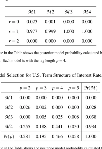
M

4 with the p=4.3 Table 3 reports the posterior model probabilities calculated by using the Schwarz BIC for

_M

1 -

_M

4, varying the lag length p=2 - 5. Clearly, nonlinearity by the Markov process is detected with almost 100 percent. The posterior model probability for

M

4 is Pr(

M

4|Y) =∑5_p=2Pr(

M

4,p|Y)≈0.934, and thus there is strong evidence to support

M

4. The highest posterior model probability is 44.1 percent given to

M

4 with p=4.

Table 4 reports the results of the posterior estimation of the parameters for

M

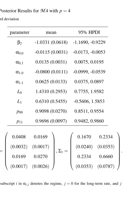
4 with p=4. From the results, the 95% HPDI ofβ(after normalizing) containsβ2=−1,

that is implied by the expectations hypothesis of the term structure. To examine whether the restriction ofβ2=−1 is appropriate in a more formal way4, we

calcu-late the Bayes factor as BF≈exp[−0.5(BICR−BICU R)], where BICU R is the unre-stricted BIC, and BICRis the restricted BIC with the restrictions of β= (1,−1), and the the value is 278.14, which shows a very strong evidence to support the expectations hypothesis.5

The posterior expectation of the state variables is plotted in Figure 2. The non-borrowed reserves operating procedure between 1979 and 1982 is detected as the regime shift. Regime shift occurs also in 1972 and 1984. These regime shifts are corresponding to higher inflation regime (Goodfriend, 1998), and are characterized by a much higher variance of both the long and the short interest rate than those of regime 0. In regime 0, that is relatively stable period, the variance of the long rate is higher than that of the short rate; on the other hand, in regime 1, the short rate fluctuates much more than the long rate. The risk premium in regime 1, L1, is lower than in regime

0, L0, that implies long run inflation expectations decrease during high inflation

pe-riod due to the central bank’s anti-inflationary monetary policy by rising the short term interest rate.

3_{We have also tested for the number of cointegration rank ofM1 -M4 with different lag length at} p=2,3,and 5, and the results are all the same as when p=4, that is, there is very strong evidence of rank 1.

4_{As Koop (2004) note, “the justification for using the HPDIs to compare models is an informal one}

which, in contrast to posterior odds, is not rooted firmly in probability theory.”

5_{See Kass and Raftery (1995) for a rule of thumb for evaluating Bayes factors. According to this rule}

of thumb, if BFi jis between 20 and 150, there is a strong evidence against model j, and if BFi jexceeds

We find that the adjustment term for the long-term rate is positive asαi,0<0 and

for the short-term rate negative asαi,1 >0 for both regimes, which implies that the

long-term rate tends to fall and the short-term rate tends to rise against the disequi-librium in either regime. The adjustment terms for both the long and the short-term rate in both regimes are significant as the 95% HPDIs for those values do not contain zero. Figure 3 plots the posterior densities for these adjustment terms and indicates that these densities do not contain zero. In regime 1 of higher volatility in the inter-est rates, the posterior mean of the adjustment speed for both the short (α1,0) and the

long rates (α1,1) is(−0.0800,0.0625)which is much faster than those in the regime 0

(α0,0,α0,1) = (−0.0115,0.0135). This implies that interest rates adjust much faster in

periods of high volatility with high inflation and anti-inflationary monetary policy.

5

Conclusion

In this paper we consider a Markov switching vector error correction model where the adjustment terms, the lag terms, the intercept terms, and the variance-covariance matrix are subject to the regime shifts with the first order unobservable Markov process while the cointegrating vector is unaffected by the regime shifts.6

Estimations are carried out entirely by a Bayesian method. The cointegrating vec-tor is drawn using the method by Strachan and Inder (2004) in a nonlinear framework so that the estimation of the cointegrating vector is more efficient than multi-step clas-sical methods where the cointegrating vector is estimated assuming the model is linear. To select the most appropriate model among linear, Markov switching, and other model specifications, we use the posterior model probabilities by approximating the Bayes factors by the Schwarz BIC. Although the Schwarz BIC does not generate the exact value of Bayes factor but just approximation, the Monte Carlo simulation show that it selects generally a correct model. To determine the number of cointegrating

6_{It is possible to allow the cointegrating vectors to change with Markov process by slight}

modifica-tion. However, we have not done this because changing the long-run relationship is not reasonable idea unless economic theory support this.

rank, we employ the Savage-Dickey density ratio to calculate the Bayes factors for zero rank against non-zero rank.

As an application to illustrate the use of the MS-VECM, we illustrate U.S. term structure of interest rates using the MS-VECM with regime dependent risk premium. We find that regime with high volatility and high speed of adjustment captures the non-borrowed reserves operating procedure during the 1979-82 and other phases of inflation scare, while the stable regime with low volatility and low speed of adjustment prevails after the mid of 80’s.

In this paper Markov switching is chosen as a switching behavior, assuming that one regime jumps to another regime suddenly at particular dates. It is of interest to consider alternative multivariate nonlinear models such as a smooth transition vector error correction models (ST-VECM) to analyze the nonlinear cointegration where the regime shifts occur not suddenly but smoothly, and compare the ST-VECM with the MS-VECM by the Bayes factors.

Appendix

A.1 Derivation of (18) and (19)

The joint prior of B,β, andΩiis given by multiplication of (4), (7) and (8) as follows:

pvec(B),β,Ω1, . . . ,Ωm.Se_T =g(β)p(vec(B))p(Se_T) m

∏

i=1 p(Ωi) ∝g(β) m

∏

i=1 |Φ_i|hi/2|Ω_i|−(hi+n+1)/2 ! |Σ_B|−1/2exp ( −1 2 " tr m

∑

i=1 Ω−1 i Φi ! +vec(B−B0)0ΣB−1vec(B−B0) (30)

The likelihood function for B,Ω1, . . .Ωm,βandSe_T is given by,

LB,β,Ω1, . . . ,Ωm,STe |Y

∝

∏

m i=1 |Ωi|−ti/2 ! exp −1 2tr ( m

∑

i=1 Ω−1 i (Yi−WiB) 0 (Yi−WiB) )! (31) = m

∏

i=1 |Ωi|−ti/2 ! exp ( −1 2 m

∑

i=1 h

vec(Yi−WiB)0(Ωi⊗Iτ)−1vec(Yi−WiB) i

)

(32)

The joint posterior for derivingΩi is given as product of the joint prior (30) and the likelihood (31) as p(vec(B),β,Ω1, . . . ,Ωm,STe |Y) ∝pvec(B),β,Ω1, . . . ,Ωm.Se_T LB,β,Ω1, . . . ,Ωm,Se_T|Y ∝g(β) m

∏

i=1 |Φ_i|hi/2|Ω_i|−(ti+hi+n+1)/2 ! |Σ_B|−1/2exp −1 2 vec(B−B0)0ΣB−1vec(B−B0) ×exp −1 2 ( m

∑

i=1 Ω−1 i (Yi−WiB)0(Yi−WiB) +Φi )! (33)

From the joint posterior (33), the conditional posterior density forΩi can be de-rived as p(Ωi|B,β,Se_T,Y) = p(vec(B),β,Ωi,Se_T |Y) p(vec(B),β,Se_T|Y) ∝p(vec(B),β,Ωi,Se_T |Y) ∝ |Ω_i|−(ti+hi+n+1)/2exp −1 2tr Ω−1 i (Yi−WiB)0(Yi−WiB) +Φi = |Ω_i|−(ti+hi+n+1)/2exp −1 2tr Ω −1 i Φ?,i (34)

whereΦ?,i= (Yi−WiB)0(Yi−WiB) +Φi. Thus, the conditional posterior ofΩi is de-rived as an inverted Wishart distribution as

Ωi|β,B,STe ,Y∼IW (Yi−WiB)

0

(Yi−WiB) +Φi,ti+hi

. (35)

With regard to the conditional posterior density for vec(B), we use the likelihood (32), instead of (31), to obtain the joint posterior as multiplying the joint prior in (30)

by (32), we have p(vec(B),β,Ω1, . . . ,Ωm,STe |Y) ∝pvec(B),β,Ω1, . . . ,Ωm.Se_T LB,β,Ω1, . . . ,Ωm,Se_T|Y ∝g(β) m

∏

i=1 |Φ_i|hi/2|Ω_i|−(ti+hi+n+1)/2 ! |Σ_B|−1/2exp −1 2 vec(B−B0)0ΣB−1vec(B−B0) ×exp ( −1 2 m

∑

i=1

vec(Yi−WiB)0(Ωi⊗Iti)−1vec(Yi−WiB)

)

(36)

From (36), we can write the key term in the last two lines as

m

∑

i=1 h vec(Yi−WiB)0(Ωi⊗Iti)−1vec(Yi−WiB) i +vec(B−B0)0ΣB−1vec(B−B0) =vec(B−B?)0M?−1vec(B−B?) +Q where Q= m

∑

i=1 h

vec(Yi)0(Ωi⊗Iti)−1vec(Yi) i

+vec(B0)0Σ−B1vec(B0)−vec(B?)0M−?1vec(B?)

M?= ( Σ−1 B + m

∑

i=1 Ω−1 i ⊗ W 0 iWi )−1 vec(B?) =M? ( Σ−1 B vec(B0) + m

∑

i=1 h (Ωi⊗Ik)−1vec Wi0Yi i ) .

For the proof of this derivation, see Appendix of Sugita (2006). Hence, the conditional posterior density for vec(B)is derived as a multivariate normal density as follows:

p(vec(B)|Ω1, . . . ,Ωm,β,STe ,Y)∝|Σ_B| −1/2 exp −1 2 vec(B−B?)0M?−1vec(B−B?) (37)

Thus, the conditional posterior distributions forΩi and B are given as (18) and (19) respectively.

A.2 The Griddy-Gibbs Sampler

The Griddy-Gibbs sampler is proposed by Ritter and Tanner (1992). This sampler can be implemented when the conditional posterior density is unknown to the researcher. The advantage of using this sampler over the importance sampler or the Metropolis-Hastings algorithm is that researcher does not have to provide an approximation of the function, that is not easy task in many cases. The disadvantage is that this sampler demands more computing time. The procedure for implementing the Griddy-Gibbs sampler is as following:

1. Before we begin the chain, we must choose the range of the grid and the number of the grid. The range should be chosen so that the generated numbers are not truncated.

2. Let vec(β)0 = (β1,β2, . . . ,βm). With an arbitrary starting value (within the up-per and the lower bound of the grid), compute f(β1|βi2,βi3, . . . ,βim,Y), where i denotes the i-th loop, over the grid(β1,1,β1,2, . . . ,β1,U), whereβ1,1is the lower

bound of the grid ofβ1, andβ1,Uis the upper bound of the grid ofβ1.

3. Compute the values G= (0,Φ2,Φ3, . . . ,ΦU)where Φj =

Z β1,j β1,1

f(β1|βi2,β3i, . . . ,βim,Y)dβ1

j=2, . . . ,U

4. Compute the normalized pdf values G_ζ=Gj/ΦU ofζ(β1|βi2,βi3, . . . ,βim,Y). 5. Draw the random numbers from the uniform density with the lower bound as

zeros and the upper bound asΦUand invert cdf G by numerical interpolation to obtain a drawβi₁fromζ(β1|βi2,βi3, . . . ,βim,Y).

6. Repeat steps 2-5 forβ2, . . . ,βm.

7. Set i=i+1 (increment i by 1) and go to step 2.

Note that integration at the step 3 can be done by the deterministic approximation such as the Simpson’s rule or the Trapezoidal rule. The Simpson’s rule approximates the integration of f(θ), based on an interpolation, such as

Z 1

0

f(θ)dθ≈1

6[f(0) +4 f(0.5) +f(1)].

Or the extended Simpson rule can be applied as, with 2n intervals of equal length d=θi−θi−1=1/2n based on 2n+1 pointsθ0=0,θ1, . . . ,θ2n=1, Z 1 0 f(θ)dθ ≈ d 3{f(θ0) +4[f(θ1) +f(θ3) +· · ·+f(θ2n−1)] +2[f(θ2) +f(θ4) +· · ·+f(θ2n)]}.

References

[1] Anderson, H. M. (1997). Transaction costs and non-linear adjustment towards equilibrium in the US treasury bill market. Oxford Bulletin of Economics and Statistics 59, 465-483.

[2] Balke, N. S. and T. B. Fomby (1997). Threshold cointegration. International Eco-nomic Review 38, 627-645.

[3] Bauwens, L. and M. Lubrano (1996). Identification restrictions and posterior den-sities in cointegrated Gaussian VAR systems. in T. B. Fomby (ed.), Advances in Econometrics 11B, Greenwich, CT: JAI press.

[4] Bauwens, L. M. Lubrano and J-F, Richard (1999). Bayesian Inference in Dy-namic Econometric Models, Oxford: Oxford University Press.

[5] Campbell, J. Y. and R. J. Shiller (1987). Cointegration and tests of present value models. Journal of Political Economy 108, 205-51.

[6] Carlin, B. P. and S. Chib (1995). Bayesian model choice via Markov Chain Monte Carlo methods. Journal of the Royal Statistical Society Series B, 57, 473-84. [7] Carter, C. K. and P. Kohn (1994). On Gibbs sampling for state space models.

Biometrika 81, 541-553.

[8] Chib, S. (1995). Marginal likelihood from the Gibbs output. Journal of the Amer-ican Statistical Association 90, 432, Theory and Methods, 1313-1321.

[9] Chib, S. and E. Greenberg (1995). Understanding the Metropolis-Hastings algo-rithm. The American Statistician 49, 327-335.

[10] Chib, S. and I. Jeliazkov (2001). Marginal likelihood from the Metropolis Hast-ings output. Journal of the American Statistical Association 96, 270-81.

[11] Clarida, R. H., L. Sarno, M. P. Taylor, and G. Valente (2006). The role of asym-metries and regime shifts in the term structure of interest rates. Journal of Busi-ness 79, 1193-1224.

[12] Clements, M. P. and A. B. Galvao (2002). Testing the expectations theory of the term structure of interest rates in threshold models. Macroeconomic Dynamics, 1-19.

[13] Doornik, J.A. (1998), OX an Object-Oriented Matrix programming Language. London: Timberlake Consultants Press.

[14] Gelfand, A. and D. Dey (1994). Bayesian model choice: asymptotics and exact calculations. Journal of the Royal Statistical Society Series B 56, 501-14. [15] Geweke, J. (1992). Evaluating the accuracy of sampling-based approaches to the

calculation of posterior moments. in Bernardo, J., J. Berger, A. Dawid, and A. Smith (eds.). Bayesian Statistics 4, 641-49. Oxford: Clarendon Press.

[16] Goodfriend, M. (1998). Using the term structure of interest rates for monetary policy. Economic Quarterly 79, Federal Reserve Bank of Richmond, 1-23. [17] Hall, S. G., Z. Psaradakis and M. Sola (1997). Switching error-correction models

of house prices in the United Kingdom. Economic Modelling 14, 517-527. [18] Hamilton, J. (1989). A new approach to the economic analysis of nonstationary

time series and the business cycle. Econometrica 57, 357-384.

[19] Hansen, B. E. and B. Seo (2002). Testing for two-regime threshold cointegration in vector error-correction models. Journal of Econometrics 110, 293-318. [20] Johansen, S. (1988). Statistical analysis of cointegrating vectors. Journal of

Eco-nomic Dynamics and Control 12, 231-54.

[21] Johansen, S. (1991). The power function for the likelihood ratio test for cointegra-tion, in J. Gruber, ed., Econometric Decision Models: New Methods of Modelling and Applications, New York: Springer Verlag, 323-335.

[22] Kass, R. E. and A. E. Raftery (1995). Bayes factors. Journal of the American Statistical Association 90, 773-795.

[23] Kim, C. J. and C. R. Nelson (1998). Business cycle turning points, a new coin-cident index and tests of duration dependence based on a dynamic factor model with regime switching. Review of Economics and Statistics, 188-201.

[24] Kim, C. J. and C. R. Nelson (2001). A Bayesian approach to testing for Markov switching in univariate and dynamic factor models. International Economic Re-view 42, 989-1013.

[25] Kleibergen, F. and H. K. van Dijk (1998). Bayesian simultaneous equation anal-ysis using reduced-rank regression. Econometric Theory 14, 701-43.

[26] Kleibergen, F. and R. Paap (2002). Priors, posteriors and Bayes factors for a Bayesian analysis of cointegration. Journal of Econometrics 111, 223-49. [27] Koop, G. (2004). Bayesian Econometrics. Wiley.

[28] Koop, G. and S. M. Potter (1999). Bayes factors and nonlinearity: evidence from economic time series. Journal of Econometrics 88, 251-281.

[29] Koop, G., R. Leon-Gonzalez and R. Strachan (2006a). Bayesian inference in a cointegrating panel data model. Working Paper, University of Leicester, UK. [30] Koop, G., R. Strachan and H. van Dijk (2006b). Bayesian approaches to

coin-tegration. in The Palgrave Handbook of Theoretical Econometrics edited by K. Patterson and T. Mills. Palgrave Macmillan.

[31] Krolzig, H. M. (1997). Markov-switching vector autoregressions. New York: Springer.

[32] Martens, M., P. Kofman and T. C. F. Vorst (1998). A threshold error-correction model for intraday futures and index returns. Journal of Applied Econometrics 13, 245-263.

[33] Paap, R., and van Dijk, H.K., (2003) Bayes Estimates of Markov Trends in Possi-bly Cointegrated Series: An Application to US Consumption and Income, Jour-nal of Business and Economic Statistics 21, 547 - 563.

[34] Psaradakis, Z., Sola, M., Spagnolo, F., (2004) forthcoming, On Markov Error-Correction Models, With an Application to Stock Prices and Dividends, Journal of Applied Econometrics 19, 69-88.

[35] Ritter. C. and M. A. Tanner (1992). Facilitating the Gibbs sampler: The Gibbs stopper and the griddy-Gibbs sampler. Journal of the American Statistical Asso-ciation 87, 861-868.

[36] Sarno, L., and G. Valente (2005). Modelling and forecasting stock returns: Ex-ploiting the futures market, regime shifts and international spillovers. Journal of Applied Econometrics 20, 345-76.

[37] Schwarz, G. (1978). Estimating the dimension of a model. Annals of Statistics 6,461-64.

[38] Shiller, R. J. (1990). The term structure of interest rate. in Friedman, B. and F. Hahn (eds). Handbook of Monetary Economics 1, North-Holland: Amsterdam. [39] Strachan, R. W. (2003). Valid Bayesian estimation of the cointegrating error

cor-rection model. Journal of Business and Economic Statistics 21, 185-95.

[40] Strachan, R. W. and H. K. van Dijk (2003a). Bayesian model selection with an uninformative prior. Oxford Bulletin of Economics and Statistics 65, 863-876. [41] Strachan, R. W. and H. K. van Dijk (2003b). The value of structural

informa-tion in the VAR. Econometric Institute Report EI 2003-17. Erasmus University Rotterdam, Rotterdam.

[42] Strachan, R. W. and B. Inder (2004). Bayesian analysis of the error correction model. Journal of Econometrics 123, 307-25.

[43] Sugita, K. (2006). Bayesian Analysis of Dynamic Multivariate Models with Mul-tiple Structural Breaks. mimeo.

[44] Tsay, R. S. (1998). Testing and modeling multivariate threshold models. Journal of the American Statistical Association 93, 1188-1202.

[45] Verdinelli, I. and L. Wasserman (1995). Computing Bayes factors using a gener-alization of the Savage-Dickey density ratio. Journal of the American Statistical Association 90, 614-618.

[46] Wang, J. and E. Zivot (2000). A Bayesian time series model of multiple structural changes in level, trend, and variance. Journal of Business and Economic Statistics 18, 374-386.

Table 1: Average posterior probabilities: Testing for Cointegration, Non-Cointegration and Markov Cointegration

True Model =

M

1 True Model =

M

2

model T=100 T=200 T =500

M

1 0.921 0.958 0.996

M

2 0.040 0.020 0.001

M

3 0.037 0.022 0.003

M

4 0.002 0.000 0.000 model T =100 T =200 T =500

M

1 0.032 0.000 0.000

M

2 0.859 0.946 0.973

M

3 0.088 0.043 0.021

M

4 0.021 0.011 0.006

True model =

M

3 True Model =

M

4

model T=100 T=200 T =500

M

1 0.065 0.044 0.006

M

2 0.024 0.021 0.001

M

3 0.897 0.935 0.993

M

4 0.012 0.000 0.000 model T =100 T =200 T =500

M

1 0.027 0.000 0.000

M

2 0.037 0.028 0.003

M

3 0.070 0.031 0.006

M

4 0.862 0.941 0.991

Note: Each element in Table shows the average posterior model probabilities calculated by using the Schwarz BIC.

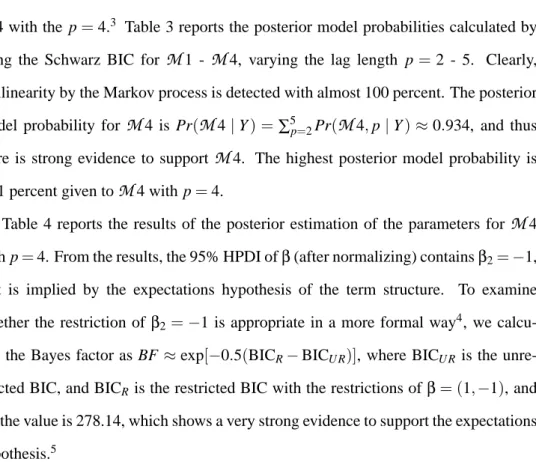
Table 2: Cointegration Test for U.S. Term Structure of Interest Rates

M

1

M

2

M

3

M

4

r=0 0.023 0.001 0.000 0.000 r=1 0.977 0.999 1.000 1.000 r=2 0.000 0.000 0.000 0.000

Note: Each value in the Table shows the posterior model probability calculated by using the Savage-Dickey density ratio. Each model is with the lag length p=4.

Table 3: Model Selection for U.S. Term Structure of Interest Rates with r=1 p=2 p=3 p=4 p=5 Pr(

M

)

M

1 0.000 0.000 0.000 0.000 0.000

M

2 0.026 0.002 0.000 0.000 0.028

M

3 0.000 0.005 0.025 0.008 0.038

M

4 0.255 0.188 0.441 0.050 0.934 Pr(p) 0.281 0.195 0.466 0.058 1.000

Note: Each value in the Table shows the posterior model probability calculated by using the SBIC. The bottom row of the Table shows the marginal probabilities for each lag length Pr(p) =∑4_i=1Pr(Mi,p). The right column of the Table shows the marginal probabilities for each model Pr(M) =∑5_p=2Pr(Mi,p).

Table 4: Posterior Results for

M

4 with p=4

( ) = standard deviation

parameter mean 95% HPDI

β2 -1.0331 (0.0618) -1.1690, -0.9229 α0,0 -0.0115 (0.0031) -0.0173, -0.0053 α0,1 0.0135 (0.0031) 0.0075, 0.0195 α1,0 -0.0800 (0.0111) -0.0999, -0.0539 α1,1 0.0625 (0.0133) 0.0375, 0.0897 L0 1.4310 (0.2953) 0.7755, 1.9582 L1 0.6310 (0.5455) -0.5606, 1.5853 p00 0.9098 (0.0270) 0.8511, 0.9554 p11 0.9696 (0.0097) 0.9482, 0.9860 Σ0=          0.0408 0.0169 (0.0032) (0.0017) 0.0169 0.0270 (0.0017) (0.0026)          ,Σ1=          0.1670 0.2334 (0.0240) (0.0353) 0.2334 0.6660 (0.0353) (0.0787)          .

Note: The subscript i inαi,j denotes the regime, j=0 for the long-term rate, and j=1 for the

Figure 1: US 3-month bill rate, 10-year bond rate and the spread

Figure 2: Posterior expectation of the regime variable E[St|Y] for th US Term Structure of Interest rates

Figure 2: Histogram of posterior densities forαfor US term structure of interest rates