Stark Contrasts in Incumbency Effects

(1)

Clemson University

TigerPrints

All Theses Theses

8-2017

Stark Contrasts in Incumbency Effects

Priyanka Prayag Jha

Clemson University, priyanj@clemson.edu

Follow this and additional works at:https://tigerprints.clemson.edu/all_theses

This Thesis is brought to you for free and open access by the Theses at TigerPrints. It has been accepted for inclusion in All Theses by an authorized administrator of TigerPrints. For more information, please contactkokeefe@clemson.edu.

Recommended Citation

Jha, Priyanka Prayag, "Stark Contrasts in Incumbency Effects" (2017).All Theses. 2706.

(2)

STARK CONTRASTS IN INCUMBENCY EFFECTS A Thesis Presented to the Graduate School of Clemson University In Partial Fulfillment

of the Requirements for the Degree Master of Arts

Economics

by

Priyanka Prayag Jha August 2016

Accepted by:

Dr. Patrick L. Warren, Committee Chair Dr. Scott Barkowski

(3)

ii ABSTRACT

Recent studies of electoral accountability show that in countries like India, Brazil and some Eastern European countries incumbents face a disadvantage compared to their challengers. These results are in contrast to evidence from the US and other western democracies where incumbents enjoy a significant advantage. In order to examine this difference in the effects of incumbency status we analyze the Indian parliamentary elections between 1998 and 2014. We use Regression Discontinuity (RD) Design to study how being an incumbent affects the contestants’ margin of victory and probability of winning in a reelection. The results from the study show that incumbents faced a consistent disadvantage over the five elections even though the level of disadvantage varied over these elections.

(4)

iii TABLE OF CONTENTS Page TITLE PAGE ... i ABSTRACT ... ii LIST OF TABLES ... ⅳ LIST OF FIGURES ... ⅴ CHAPTER I. INTRODUCTION ... 1

II. LITERATURE REVIEW ... 4

III. INDIAN POLITICAL SYSTEM ... 7

IV. DATA AND METHODOLOGY ... 10

V. RESULTS AND DISCUSSION ... 18

a. All Parties Analysis ... 18

b. Party-wise Analysis ... 26

c. Coalition-wise Analysis ... 36

VI. CONCLUSION ... 46

APPENDICES ... 48

A: Category-wise Analysis ... 49

B: Pandas Code for All Parties Analysis ... 52

C: Pandas Code for Party-wise Analysis ... 69

D: Pandas Code for Coalition-wise Analysis... 84

(5)

iv

LIST OF TABLES

Table Page

1. Snapshot of data obtained from the ECI website used in this analysis ... 11

2. The incumbency disadvantage for all parties... 20

3. The incumbency disadvantage for BJP and INC ... 27

(6)

v

LIST OF FIGURES

Figure Page

1. Adapted from Lee 2008, figure showing discontinuity at zero signifying

incumbency advantage ... 14 2. The probability of winning in 1999 as a function of the margin of victory

in 1998 ... 21 3. The probability of winning in 2004 as a function of the margin of victory

in 1998 (BJP) ... 28 7. The probability of winning in 1999 as a function of the margin of victory

in 1998 (INC) ... 29 8. The probability of winning in 2004 as a function of the margin of victory

in 1998 (NDA) ... 38 15. The probability of winning in 1999 as a function of the margin of victory

in 1998 (UPA) ... 39 16. The probability of winning in 2004 as a function of the margin of victory

(7)

vi

List of Figures (Continued)

Figure Page

20. The probability of winning in 2014 as a function of the margin of victory

in 2004 considering candidate caste ... 50 23. The probability of winning in 2014 as a function of the margin of victory

(8)

1

CHAPTER ONE INTRODUCTION

Research based on Western democracies shows that incumbent politicians (e.g. Ansolabhere et al., 2000; Cox and Katz, 1996; Erilson, 1971; Gelman and King, 1990) and political parties (Lee, 2008) demonstrate an advantage during elections at all levels of government (e.g. Ansolabhere and Snyder, 2002; Hirano and Snyder, 2009). Although most of this research is focused on U.S. elections, studies based on other Western democracies also show that incumbents have an advantage over non-incumbents in elections (e.g. Hainmueller and Lurz-Kern, 2008; Katz and King, 1999; Carey and Shugart, 1995; Ferejohn and Fiorina, 1987).

Several theories have been developed to explain this incumbency advantage. Incumbents have access to resources that their challengers do not. They can use these resources to influence public policies that make them seem more favorable to their constituents giving the incumbents a perceived valence advantage (Ashworth, 2005; Besley, 2007). They can also use their tenure in office to influence the media to gain more visibility, making them seem more ideologically aligned with their constituency (Lee, 2016). Incumbents also have the opportunity to generate resources that they can use for campaigning in forthcoming elections (Duraisamy et al., 2014). Incumbents, therefore, have the ability to influence their constituents in positive ways that can give them a considerable advantage over their challengers.

(9)

2

It is interesting to note that research on incumbency effects is primarily based on mature democracies, concentrating mainly on developed Western countries. More recent research based on younger democracies has shown that incumbents in developing countries do not enjoy an advantage, and in most cases might face a decided disadvantage. For example, studies based on countries like India (Linden, 2004; Uppal, 2009), Brazil (Klansja and Titiunik, 2013) and across post-communist democracies in eastern and Central Europe (Roberts, 2008) show that incumbents face a disadvantage compared to their challengers. Contrasting evidence in the nature of incumbency effects between developed Western countries and younger developing democracies makes it an interesting problem for further exploration.

Recent studies show that in developing countries like India, incumbents are viewed less favorably compared to their challengers. This negative perception of the incumbent’s tenure in office could be due to several reasons. For example, lack of social and political policies in favor of the constituents, lack of infrastructural developments and lack of public utilities can create dissatisfaction among the voters. Corruption on the part of office-motivated politician may also affect voter perception of incumbents adversely.

The purpose of this study is to conduct an empirical analysis of the effect of incumbency on election outcomes in India and also track changes in incumbency effects over time. We use election data from 543 constituencies over the last five national elections to check whether incumbents face a disadvantage (if any) over their challengers. Although research exists on previous elections in India (Linden, 2004; Uppal, 2009), the more recent elections have not been part of these studies. The Indian political landscape

(10)

3

has changed considerably in recent years due to increase in voter awareness and rise of regional parties. While single-party majority was the norm prior to 1991, multi-party coalition governments have become increasingly common since then. In order to study the effect of these changes on voter perception of incumbents it may be instructive to look at recent elections.

We analyze the effect of incumbency on the probability of winning by using a Regression Discontinuity (RD) design (Lee, 2001; Miguel and Zaidi, 2003). By using margin of victory for both winning and losing candidates and allowing incumbency status to be discontinuous at zero, we can study the causal effect of incumbency for candidates that have barely won the election as compared to those who have barely lost; as long as all other characteristics that can influence probability of winning for all candidates vary, on average, continuously at the zero margin (Lee, 2001). We study the effect of being an incumbent on the performance in a given election by estimating the relationship of probability of winning an election and the margin of victory in the previous election. We analyze the incumbency effects for individual political parties over the elections in 1998, 1999, 2004, 2009 and 2014. Aggregated incumbency effects for the two major political parties, namely Bharatiya Janata Party (BJP) and Indian National Congress (INC) are presented. Since India follows a Westminster type of Parliamentary system, alliances between parties are as important as the parties themselves, necessitating analysis of the coalitions formed between the political parties. Incumbency effects are thus presented for two major coalitions- the BJP-led National Democratic Alliance (NDA) and the INC-led United Progressive Alliance (UPA).

(11)

4

CHAPTER TWO LITERATURE REVIEW

Studies based on the United States Congress and other Western democracies show that incumbents are more likely to win reelections than non-incumbents (Gelman and King, 1990; Ansolabehere, Snyder and Stewart, 2000). Several theories have been proposed to explain this advantage. Incumbents can use their time in office to signal their efficiency to voters while non-incumbents do not have this opportunity. By strategic use of available resources incumbents can gain significant electoral advantage over their challengers (Ashworth, 2005; Mayhew, 1974). Designing public policy that aligns with the interests of the constituency (Cain, Ferejohn and Fiorina, 1987; Rivers and Fiorina, 1989), and using the media to strategically influence voters, incumbents can use their office to present themselves more favorably to the voters (Prior, 2006). Alternatively, incumbent advantage can also stem from the fact that rational voters assume that time spent in office makes incumbents more efficient and better able to serve the constituents than their inexperienced challengers (Ashworth and Bueno de Mesquita, 2008; Zaller, 1998). This incumbency advantage in resource-rich countries such as the United States is not restricted to legislative offices but extends to incumbents in non-legislative offices as well (Mahdavi, 2015; Lee 2016). Although these explanations for incumbency advantage seem intuitive they do not explain why incumbents in Brazil, India, post-communist Europe or Sub-Saharan Africa do not experience a similar advantage and in some cases even experience a disadvantage.

(12)

5

Recent empirical studies show evidence of incumbency disadvantage in developing countries around the world. Lee (2008), Linden (2004) and Uppal (2009) use a Regression Discontinuity technique to show that incumbents in national and state parliamentary elections were 14 to 22 percent less likely to win in re-elections. Titiunik (2009) and Klanja and Titiunik (2013) study mayoral elections in Brazil and find that an incumbent political party is 20 percent less likely to win a re-election. The sharp contrast in incumbency effects in developed and developing countries has made this an interesting problem for further research.

In spite of growing evidence existing literature does not provide many explanations for this incumbency disadvantage. Uppal (2009) studied state elections in India and found that the incumbency disadvantage can be attributed to poor government performance in provision of public goods. In constituencies that lacked essential utilities such as electricity, and fewer schools and hospitals, voters viewed incumbents less favorably and were more likely to punish them by voting against them in re-elections. This theory shows that voting behavior is influenced by their negative perception of the incumbent rather than the merit of their challengers (Eggers and Spirling, 2015; Lee, 2016). Other studies link incumbency disadvantage in developing countries to corruption on the part of office-motivated politicians. Klasnja (Forthcoming) studies mayors in Romania and shows that mayors with higher incentives to corruption faced a greater disadvantage. In studies based on Indian elections studies showed that the incumbency disadvantage stemmed from the participation of candidates with a criminal background in state elections (Aidt, Golden and Tiwari (2011).

(13)

6

Corruption seems like a plausible explanation for incumbency disadvantage as rent extraction is considered wasteful by voters and, therefore, they are less likely to vote for rent-seeking office-motivated politicians. In related research incumbency disadvantage has been shown to stem from specific institutional characteristics. For example, mayors in Brazil face a disadvantage that stems from the lack of term limits and weak political parties (Klasnja and Titiunik, 2014). Linden (2004) showed that in India there was a marked change in incumbency effects in elections before and after the 1980s. The study showed that incumbency disadvantage grew in elections after the 1980s due to the decline of the one of the most prominent political parties. While these explanations might help explain incumbency disadvantage in certain specific situations it is slightly more complicated to generalize these theories. Institutional differences and varying electoral processes make it difficult to isolate causal effects that may help explain the difference in incumbency effects in developed and developing countries.

(14)

7

CHAPTER THREE INDIAN POLITICAL SYSTEM

The legislative branch of the government of the Republic of India follows a Westminster parliamentary system, which is a bicameral system consisting of two houses: the Lok Sabha (House of the People) and the Rajya Sabha (Council of States). The Lok Sabha consists of 545 members who serve a five-year term - 543 of these members are elected directly from their respective constituencies and two are nominated by the President from the Anglo-Indian community, if in his opinion the Anglo-Indians community is not being adequately represented. The Rajya Sabha is a permanent house and can have a maximum of 250 members, and unlike the Lok Sabha, is not subject to dissolution. Most members of the Rajya Sabha are elected indirectly by state and union territory legislatures and twelve are appointed by the President of India based on contributions in various fields such as the arts, sports, science and social services. Members serve a staggered six-year term with one-third of the members retiring every two years. For the purpose of this study, we look at election data from Lok Sabha elections that are conducted by the Election Commission of India over 543 constituencies. The parliamentary system in India follows a single-tier majoritarian framework, i.e. each eligible voter in the country votes once and there is one set of elected representatives. All elections are first past the post, where the candidate that gets the highest number of votes wins the election.

(15)

8

India has a multi-party political system. All political parties are required to be registered with the Election Commission of India. The commission determines the status of the party based on set criteria. Registered political parties that are either national or state level parties enjoy certain advantages such as broadcast time on public television and radio channels. As of September 2016, there are 1761 registered political parties in India of which 7 are national-level and 48 are state-level parties. In addition to conducting the elections, the Commission also compiles detailed reports on all national and state elections. The reports include information on each constituency where elections were held. The number of candidates that contested, name of their political parties, number of votes cast, number of votes by each candidate and other statistics about the electorate.

In our study, we focus on five Lok Sabha elections from 1998 to 2014. The Indian political scenario has changed significantly over these last few decades. While election outcomes were mostly predictable prior to 1989, they have become more competitive since. The number of national and regional parties has grown in number. The number of candidates contesting in the elections has also increased significantly. Due to the competitive political climate and the involvement of state and regional parties in national politics, the dominance of a single political party or coalition has become less likely. The emergence of smaller regional political parties is a growing trend leading to candidates frequently switching party affiliations. Apart from growing competition among parties, the rise in communal tensions and caste and religion-based politics have added to the volatile nature of the elections. These changes may have significant effects on voter

(16)

9

perception of candidates and voter behavior leading to significantly different electoral dynamics.

Many studies based on the United States and other Western democracies have shown that incumbents have a higher chance of being reelected compared to non-incumbents. The incumbency advantage applied to Indian election as well, before 1989, as shown in the study by Linden (2004). However, incumbency advantage has declined after 1989 due to the factors listed previously. The trends in the few elections after 1989 studied by Linden suggest that incumbents may have faced a disadvantage in these elections. In this study, we have investigated the progression of this trend regarding the incumbency advantage/disadvantage for elections from 1998 to 2014. Specifically, we have looked at the effects of incumbency on election outcome for every constituency of the Lok Sabha for National Elections conducted in 1998, 1999, 2004, 2009 and 2014.

(17)

10

CHAPTER FOUR

DATA AND METHODOLOGY

The data has been obtained from the Election Commission of India (ECI). The ECI is an autonomous authority set up under the provision of the Constitution of India. The Commission is responsible for administering all state and national level elections and elections to the offices of the President and Vice President of India. In addition to overseeing the elections the ECI also publishes detailed reports on all the constituencies where elections were conducted. For each constituency, the reports contain the number of candidates contesting, their names and party affiliations, the number of votes won by each candidate as well as voter demographics. In this study we use data for all 543 constituencies over five general Lok Sabha elections.

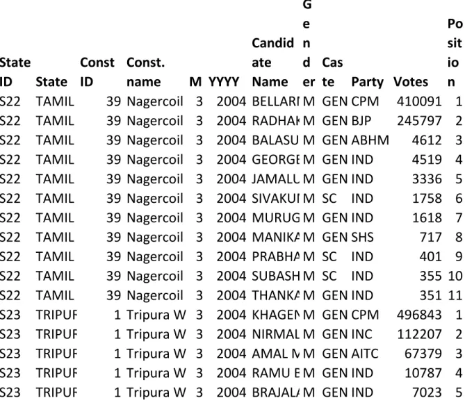
The dataset used in this study consists of detailed reports for each candidate contesting an election for each of the 543 constituencies in India. A snapshot of the data is shown in Table 1 below. Each row corresponds to one contesting candidate and lists information regarding the candidate, the constituency, party affiliation, the number of votes earned and the final position. There are typically between 5000 and 6000 rows of data for each election year. The candidates contesting the same constituency are always sorted with the winner at the top with the losing candidates following in descending order. This handy fact is utilized to identify the winner in each block of rows representing a constituency.

(18)

11

Table 1: Snapshot of data obtained from the ECI website used for this analysis

State

ID

State

Const

ID

Const.

name

M YYYY

Candid

ate

Name

G

e

n

d

er

Cas

te

Party Votes

Po

sit

io

n

S22

TAMIL NADU

39 Nagercoil 3 2004 BELLARMIN. A. V.

M GEN CPM

410091 1

S22

TAMIL NADU

39 Nagercoil 3 2004 RADHAKRISHNAN. P

M GEN BJP

245797 2

S22

TAMIL NADU

39 Nagercoil 3 2004 BALASUBRAMANIAN. T

M GEN ABHM

4612 3

S22

TAMIL NADU

39 Nagercoil 3 2004 GEORGE THOMAS. R

M GEN IND

4519 4

S22

TAMIL NADU

39 Nagercoil 3 2004 JAMALUDHEEN. B

M GEN IND

3336 5

S22

TAMIL NADU

39 Nagercoil 3 2004 SIVAKUMAR. B

M SC IND

1758 6

S22

TAMIL NADU

39 Nagercoil 3 2004 MURUGAN. V. N.

M GEN IND

1618 7

S22

TAMIL NADU

39 Nagercoil 3 2004 MANIKANTA PRASAD. M

M GEN SHS

717 8

S22

TAMIL NADU

39 Nagercoil 3 2004 PRABHAKARAN. K

M SC IND

401 9

S22

TAMIL NADU

39 Nagercoil 3 2004 SUBASH. P

M SC IND

355 10

S22

TAMIL NADU

39 Nagercoil 3 2004 THANKAMONY. C

M GEN IND

351 11

S23

TRIPURA

1 Tripura West

3 2004 KHAGEN DAS

M GEN CPM

496843 1

S23

TRIPURA

1 Tripura West

3 2004 NIRMALA DASGUPTA

M GEN INC

112207 2

S23

TRIPURA

1 Tripura West

3 2004 AMAL MALLIK

M GEN AITC

67379 3

S23

TRIPURA

1 Tripura West

3 2004 RAMU BANIK

M GEN IND

10787 4

(19)

12

Although the data obtained from ECI is detailed there are some inconsistencies that make the study of incumbency effects complicated and as such have been noted in previous works on this topic. The most significant inconsistency is found in the candidates’ names over election periods. The format in which the candidate names were recorded has changed often over the years and this makes it difficult to follow the election performance of each candidate over the years. To avoid the complications from these inconsistencies we focus our analysis on the political party as our variable of interest instead of the individual candidate.

Lok Sabha elections for the years 1998, 1999, 2004, 2009, and 2014 were examined in this analysis at the level of the constituency. The analysis was conducted party-wise instead of candidate-wise. This choice can be defended by the ansatz that the party name carries more weight in Indian elections than the candidate alone. This choice has the added benefit of avoiding any confounding factors due to inconsistencies in the reported name of the candidate.

Other inconsistencies noted in the dataset involve evolving columns across the years studied. Specifically, the name of the column denoting states has been changed from ‘state_name’ to ‘ST_NAME’ from the year 2004. The name of the column denoting the constituency was changed from ‘PC Name’ to ‘PC_NAME’ in the year 2004. The code abstracted these changing names to a name that was held constant across all years to facilitate easy analysis in ‘pandas’. A column denoting the caste of the candidate was added in 2004, while columns denoting the type of constituency and the age of the candidate were added in 2009. The insertion of these columns caused the index of the

(20)

13

columns to the right of the inserted columns to increase by 1, and due care was taken to use the appropriate index per the year in consideration. Another subtle inconsistency in the data was the presence of variable number of trailing spaces in the names of the constituencies and the name of the states reported for each candidate. The state and constituency name together form a unique identifier used to index each seat available for election in the Lok Sabha, and care needs to be taken to remove the trailing spaces to be able to match up the correct state and constituency.

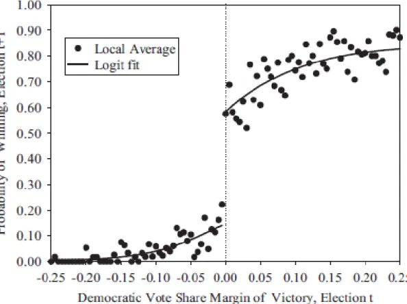
The data was analyzed in ‘pandas’ – a python framework for analyzing large datasets. The code has been reproduced in the appendices. STATA was used for polynomial regression and the subsequent Regression Discontinuity (RD) analysis, following the approach of (Lee 2008; Uppal 2009). The probability of winning of a candidate in election ‘t+1’ is plotted as a function of the margin of victory in election ‘t’. For elections where the margin of victory in election ‘t’ was huge (say > 40%), then it is conceivable and intuitively understandable that the incumbent would have, in normal circumstances, a high probability of getting re-elected. On the other hand, if a candidate lost by a huge margin in election ‘t’, then that candidate would have a low probability of winning in election ‘t+1’. One can then expect the probability of winning in election ‘t+1’ to be a continuous function of the margin of victory in election ‘t’. However, in Fig. 1 adapted from Lee (2008), that shows a similar analysis for the Democratic Party in the USA, there is an appreciable discontinuity in the probability of winning where the margin of victory is zero.

(21)

14

Figure 1: Adapted from Lee 2008, figure showing discontinuity at zero signifying incumbency advantage

(22)

15

A negative margin of victory signifies that the candidate did not win in election ‘t’, while a positive margin of victory signifies that the candidate won in both election ‘t’ and in election ‘t+1’. Thus, considering the probability of winning when the margin of victory in election ‘t’ is close to but on either side of zero, one can see that winners in election ‘t’ that have barely won enjoy a significant advantage for re-election in election ‘t+1’ as compared to losers in election ‘t’ that have barely lost. If we consider close elections, where all other factors are considered equal, then the advantage noted above is attributed to the fact that the candidate in office has favorable conditions for a successful campaign for re-election over his non-incumbent counterpart and is typically referred to as ‘incumbency advantage’, which is typically observed in Western democracies and has been well documented, as shown in Chapter 2.

For this analysis, the data was analyzed party-wise in three different ways 1. All Party analysis

2. Party-wise analysis 3. Coalition-wise analysis

All Party Analysis

The analysis is conducted using all parties contesting the particular elections. For every constituency, the margin of victory is calculated for each party that contested in that constituency. The margin of victory for all parties that did not win the constituency is the difference in the votes received by them as compared to the winning party normalized by the total votes cast in that constituency. The margin of victory for the winning party is calculated as the

(23)

16

difference in the votes received by the winner and the second-place party normalized by the total votes cast in that constituency. The margin of victory is then binned into 1% intervals and the probability of winning in election ‘t+1’ is calculated as the proportion of winners in election ‘t+1’ to the total contestants that lie in the same bin.

Party-wise Analysis:

This analysis was carried out for the two major political parties present in India – the Bharatiya Janata Party (BJP) and the Indian National Congress (INC). Only those constituencies where these two parties contested are considered for this analysis, rest were ignored. The margin of victory was calculated as follows – if the party in question (BJP or INC) was the winner in election ‘t+1’ and in election ‘t’ as well, then the margin of victory is calculated as the difference of votes received by the winning party and the second-place party normalized by the total votes cast for all candidates in that constituency. If the party in question had not won in election ‘t’, the margin of victory is calculated as the difference in the votes received by the party as compared to the winning party normalized by the total votes cast for all candidates in that constituency. Thus, the margin of victory is positive for all incumbent winners and negative for all non-incumbent winners. The margin of victory was then binned into intervals of 1%. The probability of winning was calculated as the proportion of winners belonging to the party in each bin compared to the total elections contested by the party where the margin of victory fell in the same bin.

(24)

17 Coalition-wise Analysis

The Indian political system is comprised of two major political parties and numerous smaller regional parties. However, no single political party has received the majority mandate in these election years (except 2014) to form a majority government, and thus coalitions become the driving force in the formation of a stable government. There are two major coalitions every year - the National Democratic Alliance (NDA) headed by the BJP, and the United Progressive Alliance (UPA) headed by the INC. Depending on the political climate at the end of each election, many regional parties are known to switch alliances. Thus, the party composition of each coalition changes from one election cycle to the next. The year-wise party alliances were hardcoded into the code (see appendices). For every party contesting a given constituency, the alliance was determined depending on the party and the year. Once the alliance had been determined, the rest of the analysis was similar to the analysis described in the party-wise section.

Data Fitting

The data was fitted on either side of the abscissa – the axis signifying margin of victory. As only close elections are to be considered, the fit was not smoothed over the entire range, rather only over 5 points in the local region. This was accomplished by the ‘-n’ option in the stata lpoly command. As a result, the fits appear jagged as it is not smoothed across the entire range; however, only the contributions from close elections are considered when establishing the magnitude of the discontinuity at zero.

(25)

18

CHAPTER FIVE

RESULTS AND DISCUSSION

Results are presented for the three different analyses described in the previous section. In all these plots, the ordinate is the probability of winning in election ‘t+1’ while the abscissa is the margin of victory in election ‘t’. Calculation of the two parameters has been described in the previous section.

All Parties Analysis 1. 1998-1999:

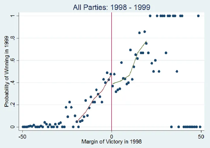
Figure 2 shows the scatter plot for the election year ‘t=1998 and ‘t+1’=1999. The election was conducted within one year of the previous election due to a coalition government losing a no-confidence motion in the Parliament following the withdrawal of a party from the coalition. As can be immediately seen in the figure, the discontinuity seen in Fig. 1 has disappeared. This signifies that the advantage enjoyed by incumbents in the Western democracies like the USA is not enjoyed by the incumbents in India. The data was restricted to within 20% margin of victory on the x-axis and a fourth degree polynomial was used for the polynomial regression following the approach of Lee (2008). The level of incumbency disadvantage is approximately 9 percentage points.

(26)

19 2. 1999-2004:

Figure 3 shows the analysis for all parties for the years 1999 – 2004. For this election, an incumbency disadvantage of approximately 30 percentage points can be observed in this data, which is consistent with all-candidates data analyzed previously (See Figure 1 in Duraisamy, Lemennicier and Khouri, 2014).

3. 2004 – 2009:

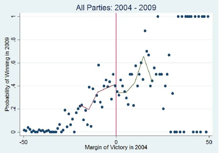
Figure 4 shows the probability of winning in 2009 as a function of the margin of victory in 2004. The discontinuity at zero has gone down to approximately 9.6 percentage points as compared to almost 30 in the last election year. This decrease in the incumbency disadvantage is consistent with the results reported in the literature. (See Figure 2 in Duraisamy, Lemennicier and Khouri, 2014)

4. 2009 – 2014:

This election year has been the most recent one in India and has not been included in the studies referenced here. Figure 5 shows the probability of winning in 2014 plotted as a function of the margin of victory in 2009. The incumbent still faced a disadvantage as compared to the incumbent in the 2009-2014 elections. The incumbency disadvantage went up to 10 percentage points in the last elections.

(27)

20

The following table summarizes the incumbency disadvantage across all years.

Table 2: Incumbency Disadvantage from 1998 to 2014

Year All Parties

1998-1999 9.1 1999-2004 29.8 2004-2009 9.6 2009-2014 10.1

(28)

21

Figure 2:The probability of winning in 1999 as a function of the margin of victory in 1998

(29)

22

(30)

23

(31)

24

(32)

(33)

26 Party-wise Analysis

Analysis for the BJP and the INC party are presented year-wise. If the Indian political system was truly a two party system, then the plots for BJP would be the complement of the plots for INC, as it would be in a zero sum game. However, the numerous regional parties in India split the vote and the two party approximations are not always valid, thus we present results for both parties separately for each year.

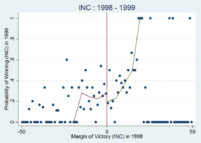
1. 1998 – 1999:

Figures 6 and 7 show the probability of winning in 1999 plotted against the margin of victory in 1998 for BJP and INC respectively.

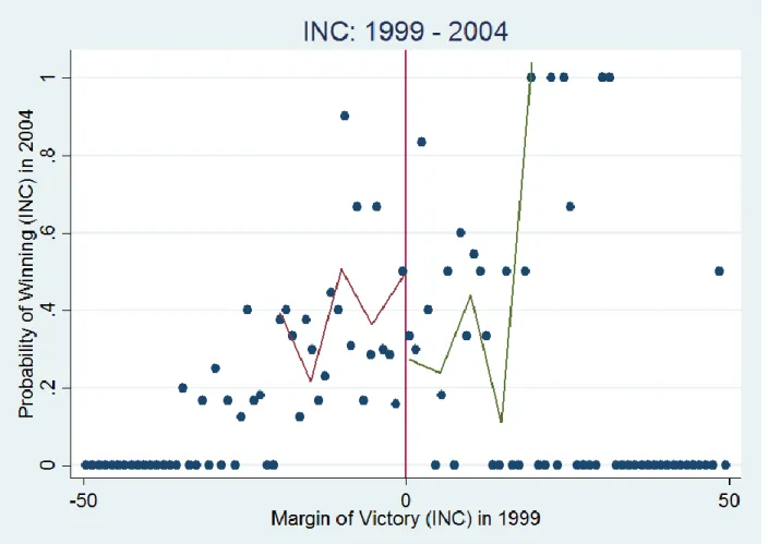
2. 1999 – 2004:

3. 2004 – 2009:

4. 2009 – 2014:

(34)

27

Table 3 summarizes the results from the RD for both parties year-wise. A positive number signifies incumbency disadvantage in percentage points, while a negative number signifies incumbency advantage in percentage points. As can be seen in the table, the incumbency disadvantage is not constant but varies year to year and across both parties. There is one instance of incumbency advantage for BJP in 2004 – 2009; however, an incumbency disadvantage is faced by both parties in every year to a varying degree.

Table 3: The incumbency disadvantage for BJP and INC

Year BJP INC

1998-1999 0.26 0.08 1999-2004 0.07 0.26 2004-2009 -0.38 0.42 2009-2014 0.06 -0.03

(35)

28

Figure 6: The probability of winning in 1998 as a function of the margin of victory in 1999 (BJP)

(36)

29

Figure 7: The probability of winning in 1998 as a function of the margin of victory in 1999 (INC)

(37)

30

(38)

31

(39)

32

Figure 10 The probability of winning in 2009 as a function of the margin of victory in 2004 (BJP)

(40)

33

(41)

34

(42)

35

(43)

36 Coalition-wise Analysis

Analysis for the NDA and the UPA alliances are presented year-wise. The BJP-led NDA and the INC-led UPA are the two major alliances that dominate the Lok Sabha elections. We present results for both alliances separately for each year.

1. 1998 – 1999:

Figures 14 and 15 show the probability of winning in 1999 plotted against the margin of victory in 1998 for NDA and UPA respectively.

2. 1999 – 2004:

3. 2004 – 2009:

4. 2009 – 2014:

Table 4 summarizes the results from the RD for both alliances year-wise. A positive number signifies incumbency disadvantage in percentage points, while a negative number signifies incumbency advantage in percentage points. As can be seen in the table, the incumbency disadvantage is not constant but varies year to year and across both alliances.

(44)

37

Table 4: The incumbency disadvantage for NDA and UPA

Year NDA UPA

1998-1999 0.06 0 1999-2004 0.23 0.09 2004-2009 -0.08 0.4

(45)

38

Figure 14: The probability of winning in 1998 as a function of the margin of victory in 1999 (NDA)

(46)

39

Figure 15: The probability of winning in 1998 as a function of the margin of victory in 1999 (UPA)

(47)

40

(48)

41

(49)

42

(50)

43

(51)

44

(52)

45

(53)

46 CHAPTER SIX CONCLUSION

In this study we have analyzed the results of five Indian parliamentary elections to determine the effect of incumbency status on the probability of winning and margin of victory of contestants using the Regression Discontinuity design. The RD design enables us to study close elections where candidates who barely won and those that barely lost can be considered to differ only in their incumbency status, thereby allowing us to study the effects of incumbency status.

The results show that there is consistently an incumbency disadvantage faced by electoral candidates in India as observed in the last five elections. The level of incumbency disadvantage varies widely year-to-year, from a few percentage points up to almost 30 percentage points. Factors such as elections being held out of cycle or after a hung parliament might affect the level of incumbency as seen in the 1998-1999 elections. Similarly, other local and national events caused incumbency disadvantage to change from 26 percent in 2004 to 10 percent in 2009. In the most recent elections in 2014 BJP had a landslide win and the incumbency disadvantage reduced to 10 percent.

Conducting this analysis on the basis of political parties instead of individual candidates helped us deal with the inconsistencies that arise due to mismatch of candidate names. Additionally, we were able to avoid the conditional dependencies of the candidate rerunning for elections in election ‘t+1’. While there are very few instances of parties not contesting consecutive elections in a constituency, they are negligible as compared to the

(54)

47

number of instances of candidates from a particular party being nominated to contest in consecutive elections.

The primary conclusion of the study is that incumbents are disadvantaged in the Indian Parliamentary elections and this disadvantage has persisted over the last few decades. Due to the contrasting nature of the results to those from countries such as the United States make this a significant study in understanding how voter behavior varies across countries. It may also be valuable to study why these differences in incumbency effects exist and how incumbent behavior affects voter perception of incumbents. These are some of the areas that can be explored in further studies on the topic of incumbency effects.

(55)

48 APPENDICES

(56)

49 Appendix A Category-wise Analysis

We have shown in the preceding sections that a definite incumbency disadvantage exists for political parties in India. To test whether this disadvantage is due to other factors, it is necessary to analyze the data looking at other classifications. Here we have analyzed the data considering the caste category of the candidate, to identify whether the caste had any contribution to the incumbency disadvantage. The data for the caste of the candidate is available since 2005, so we have analyzed the elections in 2005,2009 and 2014. Te analysis is similar to that carried out in Secion 5a, where the classification by party is replaced by a classification by the caste of the candidate.

The impact of the caste of the candidate on the incumbency effects dictates whether the shape of the graph in the case of the category-wise analysis would look similar to the shape of the graph in the party-wise analysis. The graphs for 2004-2009 and 2009-2014 are presented below in Figs. A.1 and A.2. As can be seen in the figures, there is no discontinuity observed in the graphs as for the party-wise analysis. This indicates that the caste of the candidate is not a confounding factor for the party-wise analysis carried out in the preceding sections. Similar tests for other variables should be carried out in the future to eliminate any possible confounding factors from the analysis.

(57)

50

Figure 22: The probability of winning in 2009 as a function of the margin of victory in 2004 considering candidate caste

(58)

51

Figure 23: The probability of winning in 2014 as a function of the margin of victory in 2009 considering candidate caste

(59)

52 Appendix B

Pandas Code for ‘All Parties’

# -*- coding: utf-8 -*- """

Created on Sun Jun 26 19:06:52 2016

@author: labuseruni """ import math import pandas as pd import numpy as np import matplotlib.pyplot as plt

from operator import itemgetter,attrgetter

#df_2009=pd.read_csv('2009.csv') bin_width=1.0

#set bin_width in percent margin of vote share yearlist= [ '1998','1999','2004','2009','2014'] #yearlist= [ '2009','2014']

(60)

53 partylist= ['all_parties']

for year_i in range(0,len(yearlist)-1): # year1='1998' # year2='1999' year1=yearlist[year_i]; year2=yearlist[year_i+1]; df_t1=pd.read_csv(year1+'.csv') df_t2=pd.read_csv(year2+'.csv') for partyname in partylist: #partyname='INC'

outputfile=partyname+'_'+year1+'_'+year2+'_v3.csv' outputfile2=partyname+'_'+year1+'_'+year2+'_v3.txt' #Replace space in column name with _

df_t1.columns = [c.replace(' ', '_') for c in df_t1.columns] df_t2.columns = [c.replace(' ', '_') for c in df_t2.columns]

(61)

54

#Hacks for this to work, should be more seamless using decided key-value pairs for 'interesting' columns

y2014={'statename': 'State name','pcname': 'PC Name','partyname_index': 11,'votes_index': 12,'position_index' : 13}

y2004={'statename': 'ST_NAME','pcname': 'PC_NAME','partyname_index': 10,'votes_index': 11,'position_index' : 12}

y1998={'statename': 'ST_NAME','pcname': 'PC_NAME','partyname_index': 9,'votes_index': 10,'position_index' : 11} mydict={'2014':y2014,'2009':y2009,'2004':y2004,'1999':y1999,'1998':y1998} dict1=mydict[year1] dict2=mydict[year2]

#creates new column that is unique

(62)

55 if(year1=='2009' or year1 == '2014'): df_t1['Unique']=df_t1.State_name.str.cat(df_t1.PC_name,sep='_') df_t1['Unique']=df_t1.Unique.str.replace(' ','_') df_t1['Unique']=df_t1.Unique.str.strip() df_t1['Unique']=df_t1.Unique.str.upper() else: df_t1['Unique']=df_t1.ST_NAME.str.cat(df_t1.PC_NAME,sep='_') df_t1['Unique']=df_t1.Unique.str.replace(' ','_') df_t1['Unique']=df_t1.Unique.str.strip() df_t1['Unique']=df_t1.Unique.str.upper()

#PC_names have trailing spaces! - the 'strip' removes these so we can search between different years!

if(year2=='2009' or year2 == '2014'): df_t2['Unique']=df_t2.State_name.str.cat(df_t2.PC_name,sep='_') df_t2['Unique']=df_t2.Unique.str.replace(' ','_') df_t2['Unique']=df_t2.Unique.str.strip() df_t2['Unique']=df_t2.Unique.str.upper() else: df_t2['Unique']=df_t2.ST_NAME.str.cat(df_t2.PC_NAME,sep='_') df_t2['Unique']=df_t2.Unique.str.replace(' ','_') df_t2['Unique']=df_t2.Unique.str.strip()

(63)

56 df_t2['Unique']=df_t2.Unique.str.upper() unique_vals_t1=df_t1['Unique'].unique() unique_vals_t2=df_t2['Unique'].unique() unique_vals = list(set(unique_vals_t1).intersection(unique_vals_t2)) unique_vals.sort()

#unique_vals now has id per constituency common to both years

df_t1_indexed=df_t1.set_index('Unique') df_t2_indexed=df_t2.set_index('Unique')

#alternatively, try indexing with two columns? for another day.

#for now, use arrays: a_t1=df_t1.values a_t2=df_t2.values out_a_t1=[] margins=[]

(64)

57 #unique,margin,won_flag margin_based_t1=[] count=0 for v in unique_vals: print(v) df_t1_constituency_slice=pd.DataFrame(df_t1_indexed.loc[v]) df_t2_constituency_slice=pd.DataFrame(df_t2_indexed.loc[v]) a_t1_constituency_slice=df_t1_constituency_slice.values a_t2_constituency_slice=df_t2_constituency_slice.values

#Start processing per slice i.e. per constituency total_votes=0

margin=0.0

#index to locate where in the slice the particular party we are interested in lies #assuming dataset is sorted within constituency

#if the party was a winner, this will be first pos i.e. value of indec will be 0; else non-zero

partyname_position_in_slice=-1

(65)

58 """

if(a_t1_constituency_slice[0][dict1['partyname_index']] not in partylist \ or a_t1_constituency_slice[1][dict1['partyname_index']] not in partylist \ or a_t2_constituency_slice[0][dict2['partyname_index']] not in partylist \ or a_t2_constituency_slice[1][dict2['partyname_index']] not in partylist ): #print(a_t1_constituency_slice[0][dict1['partyname_index']],a_t1_constituency_slice[1][d ict1['partyname_index']],a_t2_constituency_slice[0][dict1['partyname_index']],a_t2_cons tituency_slice[1][dict1['partyname_index']]) #wait=input() continue; """ #binary variable - # =1 if party won in t+1

# =0 if party did not win in t+1 won_flag=0; #print(a_t1_constituency_slice[0][dict1['partyname_index']],a_t1_constituency_slice[1][d ict1['partyname_index']],a_t2_constituency_slice[0][dict2['partyname_index']],a_t2_cons tituency_slice[1][dict2['partyname_index']]) count+=1

(66)

59 """ winning_partyname_in_t2=a_t2_constituency_slice[0][dict2['partyname_index']] for i in range(a_t1_constituency_slice.shape[0]): total_votes=total_votes+a_t1_constituency_slice[i][dict1['votes_index']] if(a_t1_constituency_slice[i][dict1['partyname_index']]==winning_partyname_in_t2): partyname_position_in_slice=i;

#assumption here is that there are never multiple candidates from same party contesting the same constituency

if partyname_position_in_slice==-1: continue; """ for i in range(a_t1_constituency_slice.shape[0]): total_votes=total_votes+a_t1_constituency_slice[i][dict1['votes_index']] for i in range(a_t1_constituency_slice.shape[0]): if(i==0):

(67)

60 margin=a_t1_constituency_slice[0][dict1['votes_index']]-a_t1_constituency_slice[1][dict1['votes_index']] else: margin=a_t1_constituency_slice[i][dict1['votes_index']]-a_t1_constituency_slice[0][dict1['votes_index']] margin = margin*100.0/total_votes if(a_t1_constituency_slice[i][dict1['partyname_index']]==a_t2_constituency_slice[0][dict 2['partyname_index']]): won_flag=1; else: won_flag=0; margin_based_t1.append([v+a_t1_constituency_slice[i][dict1['partyname_index']],margi n,won_flag]) """ if(partyname_position_in_slice==0):

(68)

61 margin=a_t1_constituency_slice[0][dict1['votes_index']]-a_t1_constituency_slice[1][dict1['votes_index']] won_flag=1; else: margin=a_t1_constituency_slice[partyname_position_in_slice][dict1['votes_index']]-a_t1_constituency_slice[0][dict1['votes_index']] won_flag=0; margin = margin*100.0/total_votes """ """ if(a_t2_constituency_slice[0][dict2['partyname_index']]==partyname): won_flag=1 else: won_flag=0 """ """ margin_based_t1.append([v,margin,won_flag]) """

(69)

62 #here we have generated margin_based_t1 table

#cols are unique(pc_id),margin in t1 for party, flag indicating whether party won or not in t2 #sort by margin margin_based_t1=sorted(margin_based_t1,key=itemgetter(1)) binned_margin_t1=[] for i in range(len(margin_based_t1)): bin_no=int(math.floor(abs((margin_based_t1[i][1]))/bin_width)) if(margin_based_t1[i][1]<0.0): sign_flag=-1.0 else: sign_flag=+1.0 bin_no=int(bin_no*bin_width)+bin_width/2.0 bin_no=bin_no*sign_flag print(margin_based_t1[i][1],bin_no) binned_margin_t1.append([bin_no,margin_based_t1[i][2]]) half_total_bins=int(math.ceil(100/bin_width))#one-sided total final_binned_margin=[]

(70)

63 for i in range(half_total_bins): bin_no_search1=-1.0*(i*bin_width+bin_width/2.0) bin_no_search2=+1.0*(i*bin_width+bin_width/2.0) count_won1=0 count_all1=0 count_won2=0 count_all2=0 for j in range(len(binned_margin_t1)): if(binned_margin_t1[j][0]==bin_no_search1): count_all1=count_all1+1; if(binned_margin_t1[j][1]==1): count_won1=count_won1+1; if(binned_margin_t1[j][0]==bin_no_search2): count_all2=count_all2+1; if(binned_margin_t1[j][1]==1): count_won2=count_won2+1;

(71)

64 if(count_all1!=0): final_binned_margin.append([bin_no_search1,count_won1/count_all1,count_all1,count_ won1]) else: final_binned_margin.append([bin_no_search1,0,count_all1,count_won1]) if(count_all2!=0): final_binned_margin.append([bin_no_search2,count_won2/count_all2,count_all2,count_ won2]) else: final_binned_margin.append([bin_no_search2,0,count_all2,count_won2]) final_binned_margin=sorted(final_binned_margin,key=itemgetter(0)) final_df=pd.DataFrame(final_binned_margin) final_df.to_csv(outputfile,index=False) outf=open(outputfile2,'w') for i in range(len(final_binned_margin)):

(72)

65 line=str(final_binned_margin[i][0])+"\t"+str(final_binned_margin[i][1])+"\t"+str(final_bi nned_margin[i][2])+"\t"+str(final_binned_margin[i][3])+"\n" outf.write(line) outf.close() print(year1,year2,partyname,count) wait=input() """ if(a_t2_constituency_slice[0][dict2['partyname_index']]==partyname):

(73)

66

#calculate and append BJP margin to year 't' #assuming dataset is sorted within constituency

if(a_t1_constituency_slice[0][dict1['position_index']]==1 and a_t1_constituency_slice[0][dict1['partyname_index']]==partyname): bjp_margin_t1=(a_t1_constituency_slice[0][dict1['votes_index']]-a_t1_constituency_slice[1][dict1['votes_index']]) else: for i in range(a_t1_constituency_slice.shape[0]): if(a_t1_constituency_slice[i][dict1['partyname_index']]==partyname): bjp_margin_t1=a_t1_constituency_slice[i][dict1['votes_index']]-a_t1_constituency_slice[0][dict1['votes_index']] total_votes=0 for i in range(a_t1_constituency_slice.shape[0]): total_votes=total_votes+a_t1_constituency_slice[i][dict1['votes_index']] bjp_margin_t1=bjp_margin_t1*100.0/total_votes print(bjp_margin_t1) out_a_t1.append([v,bjp_margin_t1]) margins.append(bjp_margin_t1)

(74)

67 binwidth=1.0 numbins=200/binwidth + 1.0 bins=np.linspace(-100,100,numbins) hist,bin_edges = np.histogram(margins,bins) x=bin_edges[0:numbins-1] x=x+0.5 y=hist out_df_t1=pd.DataFrame({'Count':y,'Margin':x}) out_df_t1=out_df_t1[['Margin','Count']] out_df_t1.to_csv(outputfile,index=False) plt.scatter(x,y) plt.grid() plt.plot(x,y) plt.show()

(75)

68 """ #for v in unique_vals # print(df_2009[]) #for i in range(len(a2009)): # for j in range(len(a2009[i])): # print(a2009[i][j])

#for row in df_2009[:25].itertuples(): #print(row) #for i in range(1): # for j in range(14): # print(a2009[i][j])

(76)

69 Appendix C

Pandas Code for ‘BJP/INC’

# -*- coding: utf-8 -*- """

Created on Sun Jun 26 19:06:52 2016

@author: labuseruni """ import math import pandas as pd import numpy as np import matplotlib.pyplot as plt

from operator import itemgetter,attrgetter

#df_2009=pd.read_csv('2009.csv') bin_width=1

#set bin_width in percent margin of vote share yearlist= [ '1998','1999','2004','2009','2014'] partylist= ['INC','BJP']

(77)

70 for year_i in range(0,len(yearlist)-1):

# year1='1998' # year2='1999' year1=yearlist[year_i]; year2=yearlist[year_i+1]; df_t1=pd.read_csv(year1+'.csv') df_t2=pd.read_csv(year2+'.csv') for partyname in partylist: #partyname='INC'

outputfile=partyname+'_'+year1+'_'+year2+'_v3.csv' outputfile2=partyname+'_'+year1+'_'+year2+'_v3.txt' #Replace space in column name with _

df_t1.columns = [c.replace(' ', '_') for c in df_t1.columns] df_t2.columns = [c.replace(' ', '_') for c in df_t2.columns]

#Rename column names so they arent different across years

#Hacks for this to work, should be more seamless using decided key-value pairs for 'interesting' columns

(78)

71

y1998={'statename': 'ST_NAME','pcname': 'PC_NAME','partyname_index': 9,'votes_index': 10,'position_index' : 11} mydict={'2014':y2014,'2009':y2009,'2004':y2004,'1999':y1999,'1998':y1998} dict1=mydict[year1] dict2=mydict[year2]

#creates new column that is unique

#2009&2014 have col name 'State_name', previous years have 'ST_NAME' if(year1=='2009' or year1 == '2014'):

(79)

72 df_t1['Unique']=df_t1.Unique.str.replace(' ','_') df_t1['Unique']=df_t1.Unique.str.strip() df_t1['Unique']=df_t1.Unique.str.upper() else: df_t1['Unique']=df_t1.ST_NAME.str.cat(df_t1.PC_NAME,sep='_') df_t1['Unique']=df_t1.Unique.str.replace(' ','_') df_t1['Unique']=df_t1.Unique.str.strip() df_t1['Unique']=df_t1.Unique.str.upper()

#PC_names have trailing spaces! - the 'strip' removes these so we can search between different years!

if(year2=='2009' or year2 == '2014'): df_t2['Unique']=df_t2.State_name.str.cat(df_t2.PC_name,sep='_') df_t2['Unique']=df_t2.Unique.str.replace(' ','_') df_t2['Unique']=df_t2.Unique.str.strip() df_t2['Unique']=df_t2.Unique.str.upper() else: df_t2['Unique']=df_t2.ST_NAME.str.cat(df_t2.PC_NAME,sep='_') df_t2['Unique']=df_t2.Unique.str.replace(' ','_') df_t2['Unique']=df_t2.Unique.str.strip() df_t2['Unique']=df_t2.Unique.str.upper()

(80)

73 unique_vals_t1=df_t1['Unique'].unique() unique_vals_t2=df_t2['Unique'].unique() unique_vals = list(set(unique_vals_t1).intersection(unique_vals_t2)) unique_vals.sort()

#unique_vals now has id per constituency common to both years

df_t1_indexed=df_t1.set_index('Unique') df_t2_indexed=df_t2.set_index('Unique')

#alternatively, try indexing with two columns? for another day.

#for now, use arrays: a_t1=df_t1.values a_t2=df_t2.values out_a_t1=[] margins=[] #unique,margin,won_flag margin_based_t1=[]

(81)

74 count=0 for v in unique_vals: print(v) df_t1_constituency_slice=pd.DataFrame(df_t1_indexed.loc[v]) df_t2_constituency_slice=pd.DataFrame(df_t2_indexed.loc[v]) a_t1_constituency_slice=df_t1_constituency_slice.values a_t2_constituency_slice=df_t2_constituency_slice.values

#Start processing per slice i.e. per constituency total_votes=0

margin=0.0

#index to locate where in the slice the particular party we are interested in lies #assuming dataset is sorted within constituency

#if the party was a winner, this will be first pos i.e. value of indec will be 0; else non-zero

partyname_position_in_slice=-1

"""

(82)

75

or a_t1_constituency_slice[1][dict1['partyname_index']] not in partylist \ or a_t2_constituency_slice[0][dict2['partyname_index']] not in partylist \ or a_t2_constituency_slice[1][dict2['partyname_index']] not in partylist ): #print(a_t1_constituency_slice[0][dict1['partyname_index']],a_t1_constituency_slice[1][d ict1['partyname_index']],a_t2_constituency_slice[0][dict1['partyname_index']],a_t2_cons tituency_slice[1][dict1['partyname_index']]) #wait=input() continue; """ #binary variable - # =1 if party won in t+1

# =0 if party did not win in t+1 won_flag=0; print(a_t1_constituency_slice[0][dict1['partyname_index']],a_t1_constituency_slice[1][di ct1['partyname_index']],a_t2_constituency_slice[0][dict2['partyname_index']],a_t2_const ituency_slice[1][dict2['partyname_index']]) count+=1 for i in range(a_t1_constituency_slice.shape[0]): total_votes=total_votes+a_t1_constituency_slice[i][dict1['votes_index']]

(83)

76

if(a_t1_constituency_slice[i][dict1['partyname_index']]==partyname): partyname_position_in_slice=i;

#assumption here is that there are never multiple candidates from same party contesting the same constituency

if partyname_position_in_slice==-1: continue; if(partyname_position_in_slice==0): margin=a_t1_constituency_slice[0][dict1['votes_index']]-a_t1_constituency_slice[1][dict1['votes_index']] else: margin=a_t1_constituency_slice[partyname_position_in_slice][dict1['votes_index']]-a_t1_constituency_slice[0][dict1['votes_index']] margin = margin*100.0/total_votes if(a_t2_constituency_slice[0][dict2['partyname_index']]==partyname): won_flag=1 else:

(84)

77 won_flag=0 margin_based_t1.append([v,margin,won_flag])

#here we have generated margin_based_t1 table

#cols are unique(pc_id),margin in t1 for party, flag indicating whether party won or not in t2 #sort by margin margin_based_t1=sorted(margin_based_t1,key=itemgetter(1)) binned_margin_t1=[] for i in range(len(margin_based_t1)): bin_no=int(math.floor(abs((margin_based_t1[i][1]))/bin_width)) if(margin_based_t1[i][1]<0.0): sign_flag=-1.0 else: sign_flag=+1.0 bin_no=int(bin_no*bin_width)+bin_width/2.0 bin_no=bin_no*sign_flag

(85)

78 print(margin_based_t1[i][1],bin_no) binned_margin_t1.append([bin_no,margin_based_t1[i][2]]) half_total_bins=int(math.ceil(100/bin_width))#one-sided total final_binned_margin=[] for i in range(half_total_bins): bin_no_search1=-1.0*(i*bin_width+bin_width/2.0) bin_no_search2=+1.0*(i*bin_width+bin_width/2.0) count_won1=0 count_all1=0 count_won2=0 count_all2=0 for j in range(len(binned_margin_t1)): if(binned_margin_t1[j][0]==bin_no_search1): count_all1=count_all1+1; if(binned_margin_t1[j][1]==1): count_won1=count_won1+1;

(86)

79 if(binned_margin_t1[j][0]==bin_no_search2): count_all2=count_all2+1; if(binned_margin_t1[j][1]==1): count_won2=count_won2+1; if(count_all1!=0): final_binned_margin.append([bin_no_search1,count_won1/count_all1,count_all1,count_ won1]) else: final_binned_margin.append([bin_no_search1,0,count_all1,count_won1]) if(count_all2!=0): final_binned_margin.append([bin_no_search2,count_won2/count_all2,count_all2,count_ won2]) else: final_binned_margin.append([bin_no_search2,0,count_all2,count_won2]) final_binned_margin=sorted(final_binned_margin,key=itemgetter(0)) final_df=pd.DataFrame(final_binned_margin) final_df.to_csv(outputfile,index=False)

(87)

80 outf=open(outputfile2,'w') for i in range(len(final_binned_margin)): line=str(final_binned_margin[i][0])+"\t"+str(final_binned_margin[i][1])+"\t"+str(final_bi nned_margin[i][2])+"\t"+str(final_binned_margin[i][3])+"\n" outf.write(line) outf.close() print(year1,year2,partyname,count) wait=input()