New return anomalies and new-Keynesian ICAPM

(1)

New return anomalies and new-Keynesian ICAPM

☆☆

Sungjun Cho

⁎

Manchester Business School, Crawford House, University of Manchester, Oxford Road, Manchester M13 9PL, UK

a b s t r a c t

a r t i c l e i n f o

Article history:

Received 13 February 2013

Received in revised form 15 April 2013 Accepted 25 April 2013

Available online 4 May 2013 JEL classiﬁcation:

E32 E52 G12 Keywords: New-Keynesian ICAPM Return anomalies Capital market imperfections Misspeciﬁcation-robust inference

I propose a new multi-factor asset pricing model with new-Keynesian factors to explain stock return anom-alies from 1972Q1 to 2009Q2. This new model explains the average returns across testing portfolios formed onﬁnancial distress, momentum, and standardized unexpected earnings with misspeciﬁcation-robust statis-tics. Test portfolios formed on net stock issues and total accruals are also partly explained by new-Keynesian factors. Two monetary policy factors play an important role in explaining these new anomalies. The credit as-pect of these new anomalies suggests an economic rationale for the model through capital market imperfec-tions and the credit channel of monetary policy mechanism.

1. Introduction

Fama and French (1996) demonstrate that their three-factor

model with the market excess return (RMRF) and two mimicking portfolios based on market capitalization (SMB) and book-to-market (HML) can explain the average return variations across portfolios formed on many different characteristics. They interpret their two mimicking portfolios as risk factors capturing risk premia for the relative distress ofﬁrms in the context of the ICAPM.

However, there are patterns in average stock returns that are con-sidered new anomalies because they are not explained by the Fama–

French three-factor model.Fama and French (2008)_find that the anomalous returns associated with net stock issues, accruals, and mo-mentum are pervasive in all size groups in cross-section regressions. Furthermore, Campbell, Hilscher, and Szilagyi (2008) report that more distressedfirms have lower average returns despite their high loadings on HML than less distressedfirms. They conclude that their results indicate a significant challenge to the Fama–French model.

Finally, the post-earnings-announcement drift anomaly or earnings momentum exists, ﬁrst documented by Ball and Brown (1968), which describes the outperformance of good-newsﬁrms with high standardized-unexpected earnings (SUE) relative to bad-news (low-SUE)

ﬁrms.

Recently, several papers propose commonalities in these asset pricing anomalies. For example,Avramov, Chordia, Jostova, and Philipov

(2012)ﬁnd that strategies based on price momentum, earnings

momen-tum, credit risk, and other anomalies derive their profitability from taking short positions in high credit riskfirms during the deteriorating credit conditions. WhileAvramov et al. (2012)do notfind risk-based explana-tions for the commonalities, other researchers_find connections between these anomalies and aggregate risk factors. For example,Mahajan,

Petkevich, and Petkova (2012)claim that momentum is a

compensa-tion for the systemic default risk because momentum pro_ﬁts are con-centrated in periods of high default shocks.Liu and Zhang (2008)

ﬁnd that the growth rate of industrial production is a priced risk factor for the momentum. Finally,Chen, Novy-Marx, and Zhang (2010) demon-strate that neoclassical factors based on the q-theory can explain these return anomalies. These results suggest that an asset pricing model with macroeconomic factors is a good candidate to describing these re-turn anomalies. Particularly asset pricing models with neoclassical fac-tors have a clear interpretation because the motivation of the selected factors is from equilibrium macroeconomic models.

In this paper, I add a new dimension to this literature. I argue that an Intertemporal CAPM with new-Keynesian factors motivated from new-Keynesian dynamic stochastic general equilibrium models (DSGE) is important to understand these anomalies. Like the neoclassical

☆☆ This paper is partly based on theﬁrst chapter of my doctoral dissertation at Columbia University. I am deeply indebted to Bob Hodrick, for his time, advice, and encouragement. I would also like to thank Stuart Hyde, an anonymous referee, and the editor (Brian Lucey) for helpful comments. All remaining errors are my own.

⁎Tel.: +44 161 306 3483; fax: +44 161 275 4023. E-mail address:sungjun.cho@mbs.ac.uk.

Contents lists available atScienceDirect

International Review of Financial Analysis

Open access under CC BY-NC-ND license.

(2)

approach, new-Keynesian macroeconomic analysis has micro-foundations with rational expectations. However, new-Keynesian analysis assumes a variety of market failures and emphasizes the im-portance of monetary policy actions. Surprisingly, these factors have not received deserved attention in explaining the cross-sectional asset pricing puzzles. For example, it is well known that the stock mar-ket investors continuously watches and forms expectations about the Federal Reserve Board (Fed) decisions. It seems natural to investigate the role of these monetary factors because the actions of the Fed seem to have a considerable impact on stock market returns.

However, I do not impose tight restrictions of the new-Keynesian DSGE in driving the asset pricing model with new-Keynesian factors. This reduced-form approach would induce misspecification biases naturally. To ensure robust and valid inference under the potential misspecification, I use misspecification-robust standard errors in the second pass cross-sectional regression for estimates of the risk premia or the prices of covariance risk proposed byKan, Robotti, and Shanken

(in press). They demonstrate that the statistical inference in asset

pricing models particularly with macroeconomic factors should be conducted allowing for the possibility of potential misspeciﬁcation to avoid spurious results. For the better comparison with the literature, I also report the standard errors based onFama and MacBeth (1973),

Shanken (1992), andJagannathan and Wang (1998)under correctly

specified models. As expected, the use of misspecification-robust stan-dard errors often makes a qualitative difference in determining whether estimates of the risk premia or the prices of covariance risk are statisti-cally significant, confirming the usefulness of this robust statistics. Finally, I also report standard errors of adjustedR2_following_{Kan et al.}

(in press).

The results with these robust statistical tools show that the new-Keynesian ICAPM explains the average returns of portfolios formed on_financial distress, price and earnings momentums with statistically significant adjustedR2_{. Furthermore, I}_fi_{nd that other anomalies can} be at least partially explained by these new-Keynesian factors. Partic-ularly, Ifind that the temporary monetary policy factor explains the distress and momentum premia, and the permanent monetary policy factor captures the anomalous returns on portfolios formed on SUE and total accruals. These two monetary factors also have theoretically-consistent negative risk prices because higher interest rates from monetary tightening forecast negative changes in investment opportu-nities.1_{Other factors have limited success in explaining the anomalies}

with misspeciﬁcation-robust standard errors. While the proposed new multi-factor model has a limited success in driving out some of the anomalies, the results with new-Keynesian factors look sufﬁciently encouraging to warrant further empirical investigation. At a minimum, the evidence shows that the new-Keynesian factor model is possible to shed new light on understanding the puzzling risk premia in stock markets.

One economic interpretation of the results is the capital market imperfections story.Bernanke and Gertler (1989)andKiyotaki and

Moore (1997) predict that changing credit market conditions can

have very different effects onfirms' risks and expected returns. Inter-estingly,Avramov et al. (2012)show that return anomalies such as momentum profits are restricted to high credit riskfirms and are nonexistent forfirms of high credit quality.Mahajan et al. (2012)

claim that this credit risk is a systematic risk factor. The credit channel mechanism of monetary policy describes the theory that a central bank's policy changes affect the amount of credit that banks issue to

firms and consumers for purchases, which in turn affects the real economy and return-risk characteristics offirms. Particularly, during aflight-to-quality episode (deteriorating credit conditions) external

ﬁnancing becomes harder for lower quality borrowers. Investors or banks faced with tightened balance sheet and uncertainty aversion

shift their portfolio only towards high quality borrowers. During this uncertain period, however, easier monetary policy (arguably temporary monetary policy shock) can generate much needed liquid-ity within theﬁnancial system, correspondingly changing the credit conditions.

The rest of the paper is organized as follows.Section 2presents brieﬂy the structural new-Keynesian model employed in this study.

Section 3 outlines the empirical methods. Section 4 presents the

data and discusses the cross-sectional results of the new-Keynesian factor models for portfolios formed on various anomalies.Section 5

summarizes the mainﬁndings and concludes.

2. Empirical asset pricing models

This section motivates the new-Keynesian ICAPM; theﬁrst sub-section brie_ﬂy discusses a multi-factor asset pricing model implied by new-Keynesian equilibrium models and the second subsection ex-plains the Keynesian DSGE model employed to identify new-Keynesian factors.

2.1. The pricing kernel of the new-Keynesian models

Without imposing any theoretical structure, the fundamental existence theorem ofHarrison and Kreps (1979)states that, in the absence of arbitrage, there exists a positive stochastic discount factor, or pricing kernel,Mt+ 1, such that, for any traded asset with a gross return at timetofRi,t+ 1, the following equation holds:

1¼Et Mtþ1 Ri;tþ1

h i

ð2:1Þ

whereEtdenotes the expectation operator conditional on information

available at timet.

Standard new-Keynesian macro models employ the following ex-ternal habit speciﬁcation in utility function built onFuhrer (2000).2

EtX ∞ s¼t ψs−t U Csð ;FsÞ ¼EtX ∞ s¼t ψs−t FsC 1−σ s −1 1−σ " #

whereCsis the composite index of consumption,Fsrepresents an

aggregate demand shifting factor and usually denotes asHsGswhere Hsis an external habit level andGsis a preference shock;ψdenotes

the subject discount factor andσis the inverse of the intertemporal elasticity of consumption.

Bekaert, Cho, and Moreno (2005)derive the pricing kernel

im-plied byFuhrer (2000)assuming standard log-normality and simple three-equation new-Keynesian model:

mtþ1¼ lnψ−σytþ1þðσþηÞyt− gtþ1−gt

−πtþ1 ð2:2Þ

wheremt+ 1= ln(Mt+ 1),yt+ 1is detrended log output,gt+ 1= ln(Gt+ 1) andπt+ 1is the inﬂation rate.

They express Eq.(2.2)in terms of the structural shocks in the economy.

mt_þ1¼−it−

1

2Λ′DΛ−Λ′εtþ1 ð2:3Þ where_Λ_′is a vector of prices of risks entirely restricted by the struc-tural parameters of new-Keynesian models andDis the covariance matrix of structural shocks.

The pricing kernel(2.3)is a linear combination of structural shocks to the overall economy. In this way, any new-Keynesian model can be expressed as an asset pricing model. However, strictly speaking, this

1

As described carefully byMaio and Santa-Clara (2012), any ICAPM should produce theoretically consistent risk prices.

2

I closely follow the representation given inBekaert et al. (2005). Refer to theﬁrst nine chapters inWoodford (2003)for more detailed explanations.

(3)

pricing kernel assumes constant risk premium.Bekaert et al. (2005) ar-ticulate that without either heteroskedasticity of structural shocks or time-varying market price of risk, their model essentially imposes that expectation hypothesis holds in the bond market.

One possible remedy is to adapt the external habit speciﬁcation of

Fuhrer (2000)to that ofCampbell and Cochrane (1999)and develop a

pricing kernel with time-varying risk aversion. Since time-varying risk aversion is emphasized in theﬁnance literature, this extension would be beneﬁcial for explaining asset pricing facts. Another suggestion would be introducing heteroskedasticity in the pricing kernel and struc-tural shocks. While some steps in this direction have begun to be taken only recently,3the common practice is to estimate the log-linearized economy and plug the estimates into the second-order approximation.

The easiest but perhaps ad-hoc solution is often implemented (e.g. Hordahl, Tristani, & Vestin, 2006; Rudebusch & Wu, 2004). These researchers simply ignore pricing kernel implications of their models and set the pricing kernel exogenously. Similar approaches are often employed in the empiricalﬁnance literature, too. For example, researchers employ a version of theCampbell's (1996)ICAPM with the homoskedastic volatility even though it might not have mechanisms to generate time-varying risk premium.Petkova (2006)estimates this version of the model with homoskedastic VAR to extract state variables and uses herﬁve factor“ICAPM”model to explain the value premium. Even though theoretically it is possible to modify the pricing framework in Eq.(2.3)using time-varying price of risk or heteroskedasticity, I defer these attempts to future studies.

Instead, I focus on other aspects of new-Keynesian models. Since

Smets and Wouters (2003)developed a large-scale new-Keynesian

DSGE model, these models are not only attractive from a theoretical point of view, but also are emerging as useful forecasting tools in macroeconomics because posterior odds favored these DSGE model relative to VARs estimated with a diffuse training sample prior. As explained inDel Negro, Schorfheide, Smets, and Wouters (2007), the structural VAR based on DSGE model can be used as forecasting tools.

The ICAPM intuition suggests that state variables should forecast the changing investment opportunity set in that economy. In this sense, reasonably identiﬁed state variables from the structural VAR of new-Keynesian models are natural candidates since impulse response analysis implied by these models show that each shock explains the fu-ture course of the economy consistent with the stylized facts in monetary economics. Furthermore, reassuringly, there are time series evidence to show that arguably the most important new-Keynesian factor, the monetary policy factor affect the future risk premium (e.g.Bernanke & Kuttner, 2005; Jensen, Mercer, & Johnson, 1996).4

Based on this intuition and empirical facts, I propose the following new-Keynesian ICAPM.

E Rð Þ ¼i γ0þγMβi;Mþ∑ γu kð Þ

βi;u kð Þ; ∀i ð2:4Þ

whereE(Ri) is the return of asseti,γ0is the zero beta rate,γMis the

market risk premium, andγu(k)is the price of risk for innovations in new-Keynesian factorsk. The betas are the slope coefﬁcients from the regression of returns on the innovations of new-Keynesian factors.

The model says that the expected excess return on a portfolio is described by the sensitivity of its return to the market portfolio (RMRF) and innovations in the new-Keynesian factors I extract from a new-Keynesian DSGE model.

However, there are concerns on the misspecification of these models. For example,Del Negro et al. (2007)find that while the pre-dictions of the effects of unanticipated changes in monetary policy or technology shocks derived from the new Keynesian DSGE model are not contaminated by its dynamic misspecification, some of the other

shocks would suffer from the misspecification. This misspecification problem would also affect statistical inference in the current study. To ensure robust and valid inference, I use misspeci_fication-robust standard errors in the second pass cross-sectional regression for esti-mates of the risk premia and the prices of covariance risk proposed by

Kan et al. (in press).5_{They demonstrate that the statistical inference}

in asset pricing models particularly with macroeconomic factors should be conducted allowing for the possibility of potential misspeciﬁcation to avoid spurious results. For the better comparison with the literature, I also report the standard errors based onFama and MacBeth (1973),

Shanken (1992), andJagannathan and Wang (1998)under correctly

specified models. As expected, the use of misspecification-robust stan-dard errors makes a qualitative difference in determining whether esti-mates of the risk premia or the prices of covariance risk are statistically significant, confirming the usefulness of this robust statistics.

2.2. New-Keynesian factors

I useDe Graeve (2008)as a baseline new-Keynesian DSGE model to extract new-Keynesian factors. A series of papers proposed by

Smets and Wouters (2003)incorporate a number of real and nominal

frictions to explain the persistence in the macro-economic data. Their new-Keynesian models have become a standard approach in mone-tary policy literature because of its superior_ﬁts and forecasting per-formance.6_{However, they have an exogenous ad-hoc mechanism to}

impose capital market imperfections.

De Graeve (2008)extends the Smets and Wouter model with a

plausible endogenous mechanism to generate capital market imper-fections. In his model, entrepreneurs buy the capital stock Kt+ 1 from capital goods producers at a given priceQtwith either internal

funds (net worth,Nt+ 1) and bank loans. Entrepreneurs cannot borrow at the risk-less rate because of the asymmetric information between the financial intermediary and entrepreneurs. Therefore, the bank should pay a state verification cost for monitoring entrepreneurs. In equilibrium, entrepreneurs borrow up to the point where the expected return to capital equals the cost of externalfinance.

FollowingBernanke, Gertler, and Gilchrist (1999), he assumes that the premium over the risk-free rate required by thefinancial interme-diary is a negative function of the amount of collateralized net worth. De Graevefinds that his measure of the externalfinance premium is closely related to readily available qualitative proxies of the premium such as credit standards (Lown and Morgan (2006)), and his model performs better than the Smets and Wouters model from Bayesian hypothesis tests.

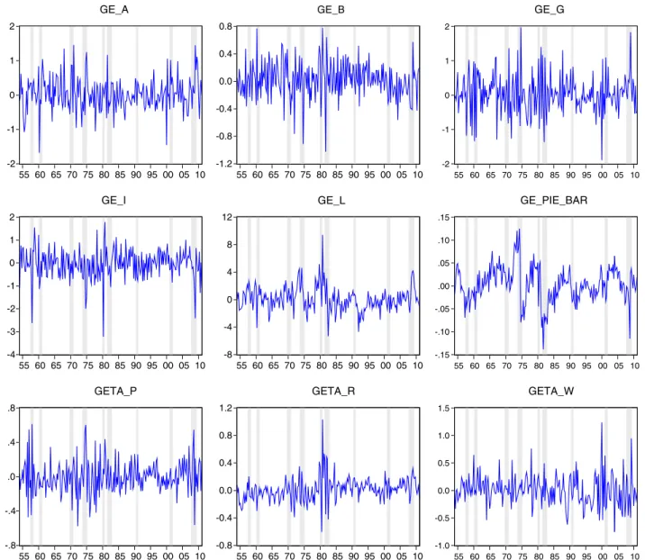
From this model, I recover the following nine structural shocks; the total factor productivity shocks (GE_A), the preference shocks (GE_B), the government spending shocks (GE_G), the shocks to invest-ment technology (GE_I), the labor demand shocks (GE_L), the perma-nent monetary policy shock (GE_PIE_BAR), the price mark-up shocks (GETA_P), the temporary monetary policy shocks (GETA_R) and the wage mark-up shocks (GETA_W).7

However, to obtain reliable empirical results using their misspeciﬁcation-robust t-statistics, Kan et al. (in press) suggest the use of small number of test assets (e.g. 30 assets). Further, given this constraint and the desire for both parsimony and for reliable statis-tical inference, it is preferable to reduce the number of factors. Here I limit the model toﬁve factors.8

Iﬁrst choose three asset pricing factors based on the theoretical arguments to minimize data mining bias. Recently,Avramov et al.

3

Refer toAn (2006)for Bayesian estimation of this type of models. 4

As explained inCampbell (1996), state variables in the ICAPM could forecast the future movement of stock returns.

5

Further details will be provided in the next section. 6

Refer toSmets and Wouters (2006)to fully understand micro-foundations of this model.

7_{Further details are provided in the}_{Appendix A.} 8

Most of factor-based asset pricing models do not seem to have more thanﬁve fac-tors. For example,Liu and Zhang (2008)useﬁve factors based onChen, Roll, and Ross (1986).

(4)

(2012)show that return anomalies are restricted to high credit risk

ﬁrms and are nonexistent forﬁrms of high credit quality.Mahajan

et al. (2012) claim that this credit risk is a systematic risk factor.

Under capital market imperfections hypothesis and the credit channel mechanism of monetary policy, the Fed's policy changes affect the amount of credit that banks issue to_ﬁrms and consumers for purchases. If the credit risk is important in explaining new return anomalies, mon-etary policy shocks and a proxy of capital market imperfections should be also important.

From the estimation of theDe Graeve's (2008)model, I obtain two monetary policy shocks and the estimated investment technology shocks. The investment technology shocks can be interpreted as the primary proxy for capital market imperfections asDe Graeve (2008)

ﬁnds that the investment technology shocks explain 85% of the exter-nalﬁnance premia. Each of these three theoretically motivated factors is discussed in the next section.

Finally, in addition to the market excess returns, afifth factor is identified via several preliminary specification analyses. More precisely, I add one shock from the remaining new-Keynesian shocks and exam-ine the statistical significance of the price of covariance risk for that additional factor. Only the preference shock seems to have independent explanatory power for some of testing portfolios while other shocks never show independent explanatory power for any asset.9_Therefore

I choose the preference shock as theﬁfth asset pricing factor.10

2.3. Digesting three new-Keynesian factors 2.3.1. Investment technology shocks

De Graeve's model has the following capital (Kt) accumulation

equation.11 Ktþ1¼Ktð1−τÞ þ 1þε I t−S Iðt=It−1Þ h i It

whereItis gross investment,τis the depreciation rate and the

adjust-ment cost functionS(It/It−1) is a positive function of changes in invest-ment. As explained inSmets and Wouters (2003),εtIis equivalent to a

shock in the relative price of investment versus consumption goods and takes up the investment speciﬁc technological shocks. The estimated results of theDe Graeve (2008)model indicate that the investment tech-nology shocks are an important determinant for the externalﬁnance premium.

Intuitively, new-Keynesian models such as De Graeve's model can be interpreted as an extension of production-based asset pricing models with short-term frictions and monetary policy. Kogan and Papanikolaou introduce new production-based asset pricing models motivated from a standard real-business cycle model with investment technology shocks.12_{These models decompose the}_ﬁ_{rm value into the}

value of assets in place and the present value of future growth opportu-nities.Kogan and Papanikolaou (in press-a)show that the investment technology shocks can explain the value premium.

Investment technology shocks affectfirms differentially depending on whether they derive most of their value from their growth opportu-nities or assets in place because investment technology shocks get implemented in the new vintages of capital. For example, a positive investment technology shock has a larger positive impact on the market value offirms that are relatively rich in growth opportunities. Intuitively, with capital market imperfections, investment shocks can affect the externalfinance premium as in De Graeve's model. For example, when

entrepreneurs are subject to binding collateral constraints, a reduction in the value of existing assets (or installed capital) reduces the value of collateral (net-worth) and thus the amount an entrepreneur can borrow, thereby increasing the externalﬁnance premium.

2.3.2. Permanent and temporary monetary policy shocks

De Graeve's model has two monetary policy shocks. The permanent monetary policy shocks reflect changes in the inflation target while the transitory shocks represent temporary deviations from the interest rate reaction function. Simpler new-Keynesian models with a single type of monetary policy shocks (e.g.Cho & Moreno, 2006) can be used by as-suming that the inflation target of monetary policy is constant, and all monetary policy actions are transient. However, recent studies such as

Coibion and Gorodnichenko (2011)ﬁnd that the inﬂation target has

been drifting over the post-WWII U.S. economic history.

Changes in the in_ﬂation target or permanent monetary policy shocks determine the persistence of measured inﬂation. SinceFriedman (1968)

initiated this literature by arguing that inflation is always and every-where a monetary phenomenon, many researchers (e.g.,De Graeve, 2008; Ireland, 2007) have used a highly persistent trend inflation pro-cess, interpreted as the Federal Reserve's slowly-moving implicit infl a-tion target, to model the sustained rise of inflation during the 1970s (the Great Inflation period) and its subsequent decline since the 1980s, and have studied its implications for various aspects of macroeconomic dynamics. Accommodative raises in the inflation target during the 1970s are often criticized as the main cause for undermining confidence in the economy and creating more volatility in the marketplace. Many re-searchers believe that the Volcker's rule with a priority for price stability in the early 1980s eventually brought both in_flation and unemployment down.

Changes in the inflation target can be an important factor for longer-term planning such as_firms' capital investment decisions. For example, if inflation expectations and actual inflation remain within a range consistent with price stability, raising the inflation target can in-duce more volatile and higher inflation, thereby undermining confidence and the ability offirms and households to make longer-term plans and squandering the Fed's inflation credibility. For this reason, the Fed has taken mostly temporary measures to ease monetary andfinancial condi-tions, through both interest rate and credit channels, during recession or crisis periods to stimulate aggregate demand and ease credit conditions. Temporary monetary easing has been the main instrument to reduce credit market imperfections and to stabilize economy.

2.3.3. Q theory and monetary policy shocks

Intuitively the neoclassical q-theory of investment (e.g.Cochrane, 1991) implies thatfirms invest more when their marginal q (the net present value of future cashflows generated from one additional unit of capital) is high. For example, given expected cashflows, low costs of capital mean high values of marginal q and high investment, whereas high costs of capital mean low values of marginal q and low investment. Because the marginal q is not observed, average q or Tobin's Q (the market value of afirm's assets relative to their replacement costs) is fre-quently used instead with constant returns to scale assumption.

Tobin (1969)argues that through the interest rate channel, the

Fed's monetary policy can play a crucial role in altering Tobin's Q. For example, a tightening of monetary policy induced by an increase in inflation lowers the present value of future earningsflows, thereby decreasing investment. Under the credit market imperfections, mon-etary policy can affect Tobin's q through credit channels, too.Hubbard (1998)summarizes two stylized facts. First, investment is significantly correlated with proxies for changes in net worth or internal funds. Sec-ond, given investment opportunities, proxies for borrowers' net worth affect investment more for lower-net-worth (orfinancially constrained) borrowers. The extended q-theory suggests that, to the extent that mon-etary policy can affect borrowers' net worth, pure interest rate effects of the Fed's monetary policy will be magnified; the more constrained the

9

Results are available upon request. 10

Because this empirically oriented approach to select a factor could induce more se-vere misspeciﬁcation biases, it is essential to rely on misspeciﬁcation-robust inference in asset pricing tests.

11_{The linearized version of this equation is provided as Eq.}_(A7)_{in the}_{Appendix A.} 12

These models also have similar capital accumulation equation with the investment technology shocks.Kogan and Papanikolaou (2012)provide an excellent survey on these models.

(5)

access to capital markets, the greater the sensitivity of investment toﬁ -nancial variables. De Graeve's model utilized in this paper includes the equivalent (linearized) version of q-theory.

3. Empirical analysis under potentially misspeciﬁed models

Following the notation ofKan et al. (in press), let's denoteftbe the

vector of K proposed asset pricing factors andRtis a vector of returns

on N test assets at timet.13

Linear beta pricing models for assetican be expressed as

E Rh ii ¼γ0þγ′1βi

whereβ′is are the multiple regression coefﬁcients ofRion the risk

fac-tors and a constant,γ0is the zero-beta rate andγ1is the vector of risk premia on the K risk factors (f). For N test assets, we can express the above equation using a compact matrix notation as

E R½ ¼Xγ

whereX= [1N,β],β= Cov[R,f]Var[f]−1is an (N × K) matrix of

fac-tor loadings andγ¼ðγ0;γ′1Þ′:

A popular approach to estimate these beta pricing models is two-pass cross-sectional regression method. The usual two-pass cross-sectional re-gression methodﬁrst estimates the betas of the N test assets by running the following multivariate regression for each time t.

Rt¼αþβftþεt; t¼1;…;T:

Let's denoteYtas [f′t,R′t]′and compute the sample mean and

covari-ance matrix ofYtas ^ μ¼ μ^1 ^ μ2 ¼1_T∑T t¼1Yt; ^ V¼ V^11 V^12 ^ V21 V^22 ¼1_T∑T T¼1ðYt−μ^ÞðYt−μ^Þ′:

The estimated betas from thisﬁrst-pass regression are given asβ^¼V^21V^

−1

11. These estimated β^s are used as regressors in the

second-pass CSR, and the zero beta rate and risk premia are given by

^

γ¼X^′X^−1X^′μ2

where X^_¼ 1N;^β

h i

and _γ_¼_½_γ0;_γ_′₁_′ is a vector consisting of the zero-beta rateð Þ_γ^0 and risk premia on the K factorsð Þγ1^ .

Researchers have typically focused on the price of the beta risk to test whether a proposed factor is priced. However,Kan et al. (in press)provide numerical examples illustrating a potential issue exists in multi-factor asset pricing models because the beta of an asset with respect to a particular factor depends on what other factors are in-cluded in thefirst-pass time-series OLS regression. Their solution to this inference problem consists in running the second-pass CSR with covariances (V^21) instead of betas.Kan et al. (in press)show that finding a statistically significant price of covariance risk is indeed ev-idence that the underlying factor isincrementally useful in explaining the cross-section of asset returns. If we let C^¼ 1N;V^21

h i

, then the price of covariance risk in the OLS regression is computed as λ^¼

^

C′C^

−1

^

C′μ2^ .

Under the correctly speciﬁed model, the asymptotic standard errors ofγ^estimates are provided byShanken (1992)andJagannathan and

Wang (1998). However, when the beta-pricing model is misspeci_ﬁed,

the asymptotic standard errors proposed by these papers are incorrect and could be misleading.Kan et al. (in press)demonstrate that the statistical inference in asset pricing models should be conducted allowing for the possibility of potential misspeciﬁcation to ensure ro-bust and valid inference.Kan et al. (in press)provide general expressions for the asymptotic variances of both γ^ and λ^ under potential model misspeciﬁcation as follows.

ffiffiffi T p ^ γ−γ ð Þ_eN0Kþ1;Vð Þγ^ where Vð Þ ¼γ^ X∞ j¼−∞ E hth′tþj h i with ht¼ðγt^−γ^Þ− ϕt^ −ϕ^ ^ γ′1V^ −1 11 ft−μ^1 ð Þ þX^_′X^−1^zt, ϕt^ ¼½γ0t;^ ðγ1t^ −ftÞ′′, ϕ^¼½γ0;^ ðγ^1−μ^1Þ′′, ^ zt¼ 0;utðft−μ^1Þ′V^ −1 11 h i ′, andut¼ μ^2−X^γ^ ′ðRt−μ^2Þ: ffiffiffi T p _^ λ−λ eN 0Kþ1;V λ^ whereV λ^ ¼ X∞ j¼−∞ E hth′tþj h i withht¼ λt^−λ^ −C^′C^−1C^′Gtλ1^ þ ^ C′C^ ₋1 ^ ztandGt ¼ðRt−μ^1Þðft−μ^2Þ′−V12:

In this two-pass regression framework,Kan et al. (in press)use, as testing assets, portfolio returns in excess of the T-bill rate, while excluding the constant from the expected return relations. This re-striction implies that the zero-beta rate is constrained to equal the risk-free rate. Without this restriction, theyﬁnd that the two-pass method produce the high values of the zero-beta rate and the negative market risk premium. However, it is well known that the zero-beta rate may be higher than the risk-free interest rate if risk-free borrowing rates exceed lending rates in the economy. Therefore it would be too re-strictive to exclude the constant and use excess returns as test assets.

Instead, I include the T-bill rate as a test asset in the regression with the constant. I have also included the Fama–French three factors as additional assets in the two-pass regressions.14_{This inclusion}

re-quires that the estimated price of risk should be consistent with the anomalies summarized in the Fama–French three-factor model. A popular goodness-of-ﬁt measure is the cross-sectionalR2_{from the} second pass regression. ThisR2_{indicates the extent to which the model's} risk measures account for the cross-sectional variation in average returns of test asset portfolios. It is deﬁned as

^ R2¼1−_^Q^ Q0 where Q^¼ê′ê, ê¼μ^2−Bγ^, Q0¼ê0′ê0 and ê0¼ IN−1Nð1′NIN1NÞ− 1 1′NIN h i ^

μ2 represent the deviations of mean returns

from their cross-sectional average.Kan et al. (in press)derive the asymp-totic distribution of under the misspeciﬁcation (0bR^2b1).

ffiffiffi T p ^ ρ2 −ρ2 eN 0;X∞ j¼∞ E ntntþj h i 0 @ 1 A where nt¼2 −utytþ1−ρ^2 vt h i ^ Q0 with ut¼ê′ðRt−μ2^ Þ, vt¼ ^ e′0ðRt−μ2^ Þ, andyt¼1−λ^′1ðft−^μ1Þ.

Finally, I conduct inference with a one-lagNewey and West (1987)

adjustment.

13

I only summarize misspeciﬁcation-robust OLS t-ratios since I only compute OLS t-ratios to explain the cross-section of original portfolio returns (return anomalies) rather than the cross-section of transformed portfolio returns (GLS) in this study. 14

(6)

4. Data and empirical results 4.1. Data

To estimate new-Keynesian factors, I use quarterly time-series of real GDP, consumption, investment, real wages, hours worked, price (GDP deﬂator), and the short-term interest rate ofSmets and Wouters

(2006)from theﬁrst quarter of 1954 to theﬁrst quarter of 2011.15

Nominal variables are_first de_flated by the GDP-de_flator and aggregate real variables are expressed in per capita terms. All variables except for hours, inflation and the interest rate are linearly detrended. I esti-mate De Graeve's model using the full sample data.

Monthly value-weighted portfolio returns on 25 portfolios sorted

byCampbell et al.'s (2008)failure probability measure and size, 25

portfolios sorted by momentum and size, 25 portfolios sorted by stan-dardized unexpected earnings (SUE) and size, 25 portfolios sorted by total accruals and size, and 25 portfolios sorted by net stock issues and size are obtained from Long Chen and transformed into quarterly series for the empirical asset pricing tests. This data span the period from 1972Q1 to 2009Q2.

The quarterly Fama–French factors (RMRF, SMB, HML) are com-puted using monthly returns of 6 portfolios formed on Size and Book-to-Market and market excess returns, T-bill rates from Kenneth French's website.16

4.2. Estimation of new-Keynesian factors

I estimateDe Graeve's (2008)model with his DYNARE program and updated data. I refer to his paper for the estimation details. Only the details on the prior selections and monitoring convergence deserve to be mentioned.

The Bayesian approach facilitates the incorporation of prior informa-tion from other macro as well as micro studies. This prior distribuinforma-tion describes the available information prior to observing the data used in the estimation. The observed data are then used to update the prior, via Bayes theorem, to the posterior distribution of the parameters.

Bayesian analysis is often criticized for its subjectivity bias from prior selections.

For the estimation of new-Keynesian models, however, informa-tive priors seem to be indispensable. Several researchers (e.g.An &

Schorfheide, 2005) criticize maximum likelihood estimation (MLE)

with“dilemma of absurd parameter estimates”when applying the MLE to DSGE models and argue that Bayesian methods often produce more acceptable parameter estimates.

For the estimation ofDe Graeve (2008), I follow his selections of prior distributions. But I experiment with several choices of non-informative priors to minimize biases caused by the selection of prior distribution. For example, with DYNARE, I can check whether posterior modes are uniquely identiﬁable with given prior density and likelihood function. I set the variance of prior density as large as possible if unique mode is identiﬁed.

In the Bayesian analysis, monitoring the convergence of parameters is critical since without it, we are not sure whether estimated parame-ters can be considered as a valid sample from the posterior distribution. Therefore, to ensure convergence, I do several checks. First, I simulate samples from the new-Keynesian model at least 200,000 draws from

ﬁve different chains and after discarding 50% of them in each chain as burn-in replications, I calculate the convergence diagnostics ofBrooks

and Gelman (1998)offered in DYNARE package. Iﬁnd every parameter

converged with this statistics. When I also draw one long chain of 1,000,000 draws from each model with 500,000 as burn-in periods, I obtain similar results.

After extensive checks, Iﬁnd that most of the parameter estimates are qualitatively similar to those presented inDe Graeve (2008),17Here I report the details on the estimated structural shocks (new-Keynesian factors) absent from the tables ofDe Graeve (2008).Table 1andFig. 1

reports the sample statistics and patterns of estimated structural shocks from De Graeve's model with updated data.

4.3. Cross-sectional implications of new-Keynesian models

In this section, I examine the pricing performance of new-Keynesian models over the period from 1972Q1 to 2009:Q2. The empirical litera-ture has uncovered several anomalous patterns (e.g.Fama & French, 2008) in the relations betweenﬁrm characteristics and stock returns that can't be explained byFama and French's (2008)three factors.

15

I thank De Graeve for sharing his DYNARE programs and data set. I closely follow De Graeve (2008)to construct the data and verify it for the common sample period. Refer to the data appendix ofSmets and Wouters (2006)andDe Graeve (2008)for more details.

16

I thank French for making his data available on line (http://mba.tuck.dartmouth. edu/pages/faculty/ken.french/data_library.html). 17

Results are available upon request. Table 1

Summary statistics for new Keynesian structural shocks.

GE_A GE_B GE_G GE_I GE_L GE_PIE_BAR GETA_P GETA_R GETA_W

Panel A: Correlation matrix

GE_A 1.0000 GE_B −0.0069 1.0000 GE_G 0.5011 −0.1380 1.0000 GE_I −0.0165 0.0331 −0.1514 1.0000 GE_L 0.1894 −0.1026 0.2474 −0.0022 1.0000 GE_PIE_BAR −0.0727 0.3175 −0.1219 0.1525 0.0959 1.0000 GETA_P −0.0572 −0.3269 0.1783 −0.1582 0.1806 0.0805 1.0000 GETA_R 0.2019 0.2548 0.2065 0.1286 0.6432 −0.1233 −0.0280 1.0000 GETA_W 0.0742 −0.0678 −0.1688 −0.0790 0.0717 0.0872 −0.0666 −0.1714 1.0000

Panel B: Univariate summary statistics

Mean 0.0318 0.0237 0.0256 −0.0430 0.1281 0.0028 −0.0035 0.0154 0.0021

Std. dev. 0.4799 0.2667 0.5746 0.6454 1.7758 0.0387 0.1924 0.1718 0.2723

Skewness 0.1235 −0.2996 0.1400 −0.9405 0.6763 −0.1548 0.3183 0.9010 0.5380

Kurtosis 4.1766 4.2986 3.9886 6.5736 6.2203 3.9786 4.2074 8.7104 4.9531

Auto(1) 0.0310 −0.1760 −0.2390 −0.0520 0.3990 0.6140 −0.1850 0.1120 0.0100

Summary statistics for structural shocks from a new-Keynesian DSGE model from 1954:1 to 2011:1. The Auto(1) give theﬁrst autocorrelation. Note: GE_A is the estimated tech-nology shocks; GE_B is the estimated preference shocks; GE_G is the estimated government spending shocks; GE_I is the estimated shocks to investment techtech-nology; GE_L is the estimated labor demand shocks; GE_PIE_BAR is the estimated shocks to the inﬂation target set by the Federal reserve(permanent monetary policy shocks); GETA_P is the estimated price mark-up shocks; GETA_R is the estimated temporary monetary policy shocks; and GETA_W is the estimated wage mark-up shocks.

(7)

In this paper, I choose, as testing assets, the anomalous returns associated with net stock issues, accruals, and price momentum, the

ﬁnancial distress anomaly, and the post-earnings-announcement drift anomaly (earnings momentum). I brieﬂy summarize the failure of the Fama–French model on these puzzles as follows.

4.3.1. A summary of return anomalies

4.3.1.1. Price and earnings momentum.Chordia and Shivakumar (2006)

examine the relation between price and earnings momentums. From time-series tests, theyﬁnd that the Fama–French model produces a signif-icant alpha for both momentums. Moreover the Fama–French model ex-acerbates momentum; losers load more on SMB and HML than winners.

4.3.1.2. Distress anomaly.Campbell et al. (2008)find that more dis-tressedfirms earn lower average returns than less distressedfirms. Controlling for risk with the Fama–French model exacerbates the anomaly because more distressedfirms appear riskier with higher loadings on SMB and HML. The magnitude of the drift is particularly larger for smallfirms.

4.3.1.3. Net stock issues. Lyandres, Sun, and Zhang (2008) ﬁnd that strong evidence of underperformance following initial public offerings, seasoned equity offerings, and convertible debt offer-ings. For example, from time-series asset pricing tests for the seasoned equity offering portfolios, they ﬁnd that the equal-weighted alpha from the Fama–French model is −0.39% per month (t =−3.52), and the value-weighted alpha is similar in magnitude.

4.3.1.4. Accruals.Wu, Zhang, and Zhang (2010) ﬁnd that accruals are positively related to current returns and negatively related to future returns. From time-series asset pricing tests for the low-minus-high total accruals portfolio, they ﬁnd that the equal-weighted alpha from the Fama–French model is 0.8% per month (t = 5.8), and the value-weighted alpha is similar in magnitude.

To understand how these patterns arise and their link to the fundamental factors of the economy, several asset pricing models are proposed based on economic models with production or credit conditions. Particularly, many papers use the q-theory to explain

-2 -1 0 1 2 55 60 65 70 75 80 85 90 95 00 05 10 GE_A -1.2 -0.8 -0.4 0.0 0.4 0.8 55 60 65 70 75 80 85 90 95 00 05 10 GE_B -2 -1 0 1 2 55 60 65 70 75 80 85 90 95 00 05 10 GE_G -4 -3 -2 -1 0 1 2 55 60 65 70 75 80 85 90 95 00 05 10 GE_I -8 -4 0 4 8 12 55 60 65 70 75 80 85 90 95 00 05 10 GE_L -.15 -.10 -.05 .00 .05 .10 .15 55 60 65 70 75 80 85 90 95 00 05 10 GE_PIE_BAR -.8 -.4 .0 .4 .8 55 60 65 70 75 80 85 90 95 00 05 10 GETA_P -0.8 -0.4 0.0 0.4 0.8 1.2 55 60 65 70 75 80 85 90 95 00 05 10 GETA_R -1.0 -0.5 0.0 0.5 1.0 1.5 55 60 65 70 75 80 85 90 95 00 05 10 GETA_W

Fig. 1.Estimated factor innovations from a new-Keynesian DSGE (1954:1–2011:1). Thisﬁgure plots the quarterly time series of smoothed structural shocks estimated by the

new-Keynesian DSGE. Note: GE_A is the estimated technology shocks; GE_B is the estimated preference shocks; GE_G is the estimated government spending shocks; GE_I is the estimated shocks to investment technology; GE_L is the estimated labor demand shocks; GE_PIE_BAR is the estimated shocks to the inﬂation target set by the Federal reserve (permanent monetary policy shocks); GETA_P is the estimated price mark-up shocks; GETA_R is the estimated temporary monetary policy shocks; and GETA_W is the estimated wage mark-up shocks. Shared areas indicate NBER business recessions.

(8)

the cross-sectional pattern in returns. For example,Chen et al. (2010)

motivate their empirical factors based on the_ﬁrst-order condition of

firms, which relates three endogenous variables offirms: the optimal investment rate, the expected futurefirm profitability, and the expected future stock return. However,Kogan and Papanikolaou (2012)criticize this approach because thisfirst-order condition has no causal content, and therefore offer no explanation about the economic causes of the re-turn anomalies.

Kogan and Papanikolaou (in press-b)also propose a uniﬁed

expla-nation for several apparent anomalies in the cross-sectional relation between average stock returns andfirm valuation ratios, past investment, profitability, market beta, or idiosyncratic volatility. Using a calibrated structural model, they argue that these characteristics are imperfect proxies for the share of growth opportunities tofirm value and that re-turn differences among_firms sorted on these characteristics are largely driven by one factor related to investment technology shocks. However, this result is not without controversy. For example,Garlappi and Song (2012)find only weak support for the existence of a significant price of risk for investment-specific shocks for the value and momentum premiums.

In this paper, I add a new dimension to this literature. I argue that an Intertemporal CAPM with new-Keynesian factors motivated from new-Keynesian dynamic stochastic general equilibrium models (DSGE) is important to understand these anomalies. Intuitively, new-Keynesian models can be interpreted as an extension of these models with short-term frictions and monetary policy actions. Surprisingly, these factors have not received deserved attention in explaining the cross-sectional asset pricing puzzles. For example, it seems natural to investigate the role of these monetary factors because the actions of the Fed seem to have a considerable impact on stock market returns.

Finally, new-Keynesian models as an extension of reduced form asset pricing models based on real business cycle models (e.g.Chen et al.,

2010) can provide more robust results with this general setting. In the next section, I present the estimation results of the new-Keynesian ICAPM and theFama and French (1993)three-factor model in explaining each puzzle and demonstrate how much the new-Keynesian factors can improve on the Fama–French factors.

4.3.2. Financial distress

Table 2 presents the estimation results of the new-Keynesian

ICAPM and theFama and French (1993)three-factor model using quar-terly value-weighted returns of the 25 portfolios sorted byCampbell et al.'s (2008)failure probability measure and size. I also include the T-bill rate and the Fama_–French three factors (in return forms by adding the T-bill rate to each factor) as additional test assets to obtain reasonable zero-beta rate and the risk premia.18_{I report estimates of}

the risk premia in Panel A and the prices of covariance risk in Panel B

with Fama and MacBeth (1973) t-ratio under correctly speciﬁed

models, theShanken (1992)and theJagannathan and Wang (1998)

t-ratio under correctly speciﬁed models that account for the EIV prob-lem andKan et al.'s (in press)model misspeciﬁcation-robust t-ratios. To show the overall usefulness of the model, I report the adjustedR2 with its standard error. Finally, I conduct every inference with a one-lag

Newey and West (1987)adjustment.19

Panel B inTable 2shows that the Fama–French three factors clearly fail to explain the returns of the 25 portfolios sorted byCampbell et al.'s Table 2

Estimates and t-ratios of zero-beta rate and risk premia on 25 size-failure portfolios with T-bill rate and three Fama–French factors (1976Q1–2009Q2). Panel A. The new Keynesian ICAPM

SF25 Constant RMRF Preference Invest.Tech Tem.Mon Per.Mon R2

(S.E.) Beta risk 1.74 1.13 −0.58 0 −0.43 −0.05 0.74 (0.27) FM 10.94 1.45 −6.21 0 −6.43 −5.74 Shanken 3.46 1.18 −2.02 0 −2.1 −1.97 JW 3.86 1.3 −2.39 0 −2.54 −2.41 Misspe 2.77 1.07 −2.95 0 −2.91 −1.26 Covariance risk 1.74 −0.06 −4.75 0.96 −11.57 −30.07 FM 10.94 −3.12 −3.57 1.53 −5.87 −4.89 Shanken 3.46 −0.98 −1.12 0.48 −1.83 −1.53 JW 3.86 −1.36 −1.16 0.63 −2.3 −1.6 Misspe 2.77 −1.22 −1.23 0.3 −2.26 −1.14

Panel B. The Fama–French three factor model

SF25 Constant RMRF SMB HML R2 (S.E.) Beta risk 3.81 −0.9 0.38 0.65 0.08 (0.14) FM 10.46 −1.05 0.8 1.02 Shanken 10.3 −1.05 0.8 1.01 JW 10.02 −1.06 0.76 0.92 Misspe 7.49 −1.03 0.68 0.31 Covariance risk 3.81 −0.02 0.03 0.01 FM 10.46 −1.03 1.27 0.65 Shanken 10.3 −1.01 1.24 0.64 JW 10.02 −0.99 1.14 0.6 Misspe 7.49 −0.71 0.98 0.2

The table presents the estimation results of two asset pricing models (Panel A: the new-Keynesian ICAPM and Panel B: the Fama–French three factor model). These models are estimated using the value-weighted returns on 25 portfolios sorted byCampbell et al.'s (2008)failure probability measure and size, T-bill rate, and the Fama–French three factors in return forms (T-bill rates are added to each factor) from 1976Q1 to 2009Q2. FollowingKan et al. (in press), I report theFama and MacBeth (1973)t-ratio under correctly specified models (FM), theShanken (1992)and theJagannathan and Wang (1998)t-ratio under correctly specified models that account for the EIV problem (Shanken and JW, respectively), and their model misspecification-robust t-ratios (Misspe). As a model diagnostic, I also report AdjustedR2

and its standard errors computed as inKan et al. (in press). I use Newey–West correction with one lag to compute all the statistics. The quarterly Fama–French factors (RMRF, SMB, HML) are computed using monthly returns of 6 portfolios formed on Size and Book-to-Market and market excess returns, T-bill rates from Kenneth French's website. Quarterly value-weighted returns on 25 size and failure probability measure portfolios are com-puted using corresponding monthly returns obtained from Long Chen. Four structural shocks are estimated from a new-Keynesian DSGE model; Preference is the estimated preference shocks; Invest.Tech is the estimated shocks to investment technology; permanent monetary policy shock (Per.Mon) and temporary monetary policy shock (Tem.Mon).

18

If I don't include the T-bill rate and the Fama–French factors as additional assets, I often estimate 12% zero-beta rate in annual terms and negative market risk premia or even negative HML premia. In asset pricing tests with the T-bill rate and the Fama–French three factors, zero-beta rates becomes reasonable (annual 6%) and the estimated risk premia remain positive in most cases. I report the results with sensible zero-beta rate and risk premia.

19

I thank Raymond Kan for sharing his matlab programs to compute misspeciﬁ cation-robust statistics.

(9)

(2008)failure probability measure and size. The adjustedR2_{is practically} zero and the estimated premium on the three factors is insigniﬁcant even with theFama and MacBeth (1973)t-ratio under correctly speci_ﬁed models.

The new-Keynesian ICAPM factors improve dramatically on the Fama_–French model. In Panel A ofTable 2, the adjustedR2_{is 74%} and statistically significant at 1% level. The estimated premia on the preference shock and the temporary monetary shock, and the permanent monetary shock are statistically significant with Shanken, Jagannathan and Wang standard errors under correctly specified models. However, once I use misspecification-robust standard errors, only the preference shocks and temporary monetary policy shocks are statistically significant with t-ratio−2.95 and−2.91, respectively.

As discussed inKan et al. (in press), only the price of covariance risk can identify factors that improve the explanatory power of the expected return. The price of covariance risk for preference shocks is not statistically significant with all t-statistics. However, the temporary monetary factor maintains its significance with misspecification-robust t-statistics₋2.26. Results for the prices of covariance risk imply that the temporary monetary policy shocks have explanatory power for the cross-section of expected returns for the test assets beyond any factor included in the model. This indicates that the typical test results on whether a factor is priced or not can lead to erroneous conclusions on the usefulness of a factor.

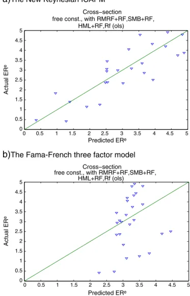
Fig. 2plots the realized versus predicted returns of the models

examined. The closer a portfolio lies on the 45-degree line, the better the model can explain the returns of the portfolio. It can be seen from the graph that the multi-factor model with new-Keynesian factors explains theﬁnancial distress premium much better than the Fama–

French three-factor model.

4.3.3. Momentum

ICAPM and the Fama and French (1993)three-factor model using quarterly value-weighted returns of the 25 portfolios sorted by prior returns and size. As before I include the T-bill rate and the Fama–French three as additional test assets to obtain reasonable zero-beta rate and the risk premia. I report estimates of the risk premia in Panel A and the prices of covariance risk in Panel B withFama and MacBeth (1973)t-ratio, the

Shanken (1992)and theJagannathan and Wang (1998)t-ratio andKan

et al.'s (in press)model misspeciﬁcation-robust t-ratios. Finally, I report the adjustedR2_{with its standard error. As before I conduct every} infer-ence with a one-lagNewey and West (1987)adjustment.

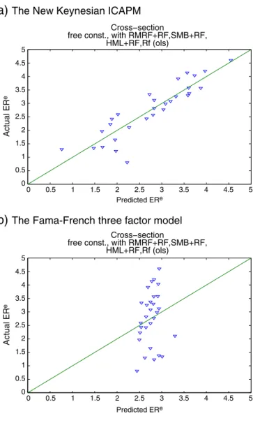
The results reported inTable 3and plotted inFig. 3 are almost same with the results inTable 2andFig. 2. Panel B inTable 3shows that the Fama–French three factors clearly fail to explain the returns of the 25 portfolios sorted by prior returns and size. The adjustedR2 is practically zero and the estimated premiums on the three factors are insigniﬁcant even with the wrong negative sign.

The new-Keynesian ICAPM factors improve dramatically on the Fama–French model. The adjustedR2is 72% and statistically signifi -cant at 1% level. The estimated premia and the price of covariance risk on the temporary monetary shock are statistically significant with misspecification-robust t-statistics−1.97 and−2.26, respectively.Fig. 3

also indicates that the multi-factor model with new-Keynesian factors explains the momentum premium much better than the Fama–French three-factor model.

4.3.4. Earnings momentum

ICAPM and the Fama and French (1993)three-factor model using quarterly value-weighted returns of the 25 portfolios sorted by stan-dardized unexpected earnings and size. Again I include the T-bill rate and the Fama–French three as additional test assets and report esti-mates of the risk premia in Panel A and the prices of covariance risk in Panel B withFama and MacBeth (1973)t-ratio, theShanken (1992)

and the Jagannathan and Wang (1998)t-ratio andKan et al.'s (in press)model misspeciﬁcation-robust t-ratios. And I report the adjusted

R2_{with its standard error as usual. Finally, I use a one-lag}_{Newey and}

West (1987)adjustment.

Panel B inTable 4again shows that the Fama–French three factors clearly fail to explain the returns of the 25 portfolios sorted by SUE and size. The adjustedR2_{is again practically zero and the estimated} premiums on the three factors are insigniﬁcant with any t-statistics.

The new-Keynesian ICAPM factors seem to improve on the Fama–

French model. In Panel A ofTable 4, the adjustedR2_{is 48% and} statis-tically signiﬁcant at 1% level whileFig. 4does not seem to show much

0 0.5 1 1.5 2 2.5 3 3.5 4 4.5 5 0 0.5 1 1.5 2 2.5 3 3.5 4 4.5 5 Cross−section

free const., with RMRF+RF,SMB+RF,

Predicted ERe

Actual ER

e

a)

The New Keynesian ICAPM

0 0.5 1 1.5 2 2.5 3 3.5 4 4.5 5 0 0.5 1 1.5 2 2.5 3 3.5 4 4.5 5 Cross−section

Actual ER

e

b)

The Fama-French three factor model

HML+RF,Rf (ols) HML+RF,Rf (ols)

Fig. 2.Fitted expected returns versus average realized returns for 25 portfolios sorted

by failure probability measure and size, T-bill, Fama–French three factors (1976Q1–

2009Q2). The plot shows realized average returns (in percent) on the vertical axis andfitted expected returns (in percent) on the horizontal axis. Two asset pricing models (the new-Keynesian ICAPM and the Fama–French three factor model) are esti-mated using the value-weighted returns on 25 portfolios sorted byCampbell et al.'s (2008)failure probability measure and size. For each portfolio, the realized average re-turn is the time-series average of the portfolio rere-turn and thefitted expected return is thefitted value for the expected return from the corresponding model. The straight line is the 45-degree line from the origin. The quarterly Fama–French factors (RMRF, SMB, HML) are computed using monthly returns of 6 portfolios formed on Size and Book-to-Market and market excess returns, T-bill rates from Kenneth French's website. Quarterly value-weighted returns on 25 size and failure probability measure portfolios are computed using corresponding monthly returns obtained from Long Chen. Four structural shocks are estimated from a new-Keynesian DSGE model; Preference is the estimated preference shocks; Invest.Tech is the estimated shocks to investment tech-nology; permanent monetary policy shock (Per.Mon) and temporary monetary policy shock (Tem.Mon).

(10)

difference between the two models. The estimated premia on the per-manent monetary shocks is statistically significant with Shanken, Jagannathan and Wang standard errors under correctly specified models. However, with misspecification-robust standard errors, the permanent monetary policy shocks lose its statistical significance. However, as explained before only the price of covariance risk can identify factors that improve the explanatory power of the expected return. The price of covariance risk for the permanent monetary policy shocks is at least marginally statistically significant with misspecification-robust t-statistics−1.89.

4.3.5. Total accruals

ICAPM and theFama and French (1993)three-factor model using quarterly value-weighted returns of the 25 portfolios sorted by total accruals and size. Again I include the T-bill rate and the Fama–French three factors as additional test assets and report estimates of the risk premia in Panel A and the prices of covariance risk in Panel B with

Fama and MacBeth (1973) t-ratio, the Shanken (1992) and the

Jagannathan and Wang (1998)t-ratio and Kan et al.'s (in press)

model misspeciﬁcation-robust t-ratios. And I report the adjustedR2 with its standard error as usual. Finally, I use a one-lagNewey and West

(1987)adjustment.

The results reported inTable 5and plotted inFig. 5show that the Fama–French three factors can capture the value-weighted returns of the 25 portfolios sorted by SUE and size comparable to the new-Keynesian model. The adjustedR2_{s are 0.68 for the new-Keynesian model and 0.65} for the Fama–French model with statistical signiﬁcance. In Panel A of

Table 5, the estimated premia on the permanent monetary shocks is sta-tistically significant at 1% with Shanken, Jagannathan and Wang standard errors under correctly specified models, but it is marginally significant

with misspecification-robust t-statistics−1.88. However, the price of covariance risk for the permanent monetary policy shocks is not statistically significant with misspecification-robust t-statistics−1.65. In Panel B ofTable 5, the estimated premia and the price of covariance risk on the HML factor are statistically significant with misspecifi cation-robust t-statistics 2.3 and 2.45 respectively.

To further investigate the relative performance of asset pricing factors in these models, I combine all factors and re-estimate the risk premia and the price of covariance risk jointly.Table 6presents the estimation results of the new-Keynesian ICAPM augmented with two Fama–French factors (the SMB and HML factors). In short, the risk premia and the price of covariance risk of the permanent monetary pol-icy shocks are statistically significant with misspecification-robust t-statistics while the price of covariance risk for the HML factor loses its statistical significance. This evidence seem to indicate that only the permanent monetary shocks provide an independent explanatory power in the cross-section of expected return of portfolios sorted by total accruals and size.

4.3.6. Net stock issues

ICAPM and theFama and French (1993)three-factor model using quarterly value-weighted returns of the 25 portfolios sorted by net stock issues and size. As before I include the T-bill rate and the Fama–French three as additional test assets and report estimates of the risk premia in Panel A and the prices of covariance risk in Panel B withFama and MacBeth (1973)t-ratio, theShanken (1992)and

theJagannathan and Wang (1998)t-ratio andKan et al.'s (in press)

model misspeciﬁcation-robust t-ratios. And I report the adjustedR2

with its standard error as usual. Finally, I use a one-lagNewey and

West (1987)adjustment.

Table 3

Estimates and t-ratios of zero-beta rate and risk premia on 25 size-momentum portfolios with T-bill rate and three Fama–French Factors (1972Q1–2009Q2). Panel A. New Keynesian ICAPM

SM25 Constant RMRF Preference Invest.Tech Tem.Mon Per.Mon R2

(S.E.) Beta risk 2.13 0.99 −0.5 0.21 −0.42 −0.02 0.72 (0.28) FM 10.35 1.25 −3.45 0.74 −4.45 −1.29 Shanken 3.7 1.08 −1.25 0.27 −1.61 −0.48 JW 2.44 1.01 −1.26 0.26 −1.68 −0.48 Misspe 2.07 0.97 −1.21 0.18 −1.97 −0.42 Covariance risk 2.13 −0.07 −3.87 1.46 −10.82 −8.61 FM 10.35 −3.47 −1.96 2.02 −4.63 −1.06 Shanken 3.7 −1.23 −0.7 0.72 −1.64 −0.38 JW 2.44 −1.36 −0.73 0.65 −1.87 −0.41 Misspe 2.07 −1.62 −0.67 0.53 −2.26 −0.43

Panel B. Fama–French three factor model

SM25 Constant RMRF SMB HML R2 (S.E.) Beta risk 2.94 −0.4 0.36 −0.04 0.03 (0.08) FM 8.96 −0.46 0.68 −0.06 Shanken 8.92 −0.46 0.68 −0.06 JW 8.31 −0.47 0.69 −0.06 Misspe 6.1 −0.48 0.56 −0.03 Covariance risk 2.94 −0.01 0.02 0 FM 8.96 −0.74 0.94 −0.23 Shanken 8.92 −0.74 0.93 −0.23 JW 8.31 −0.73 0.91 −0.21 Misspe 6.1 −0.51 0.68 −0.11

The table presents the estimation results of two asset pricing models (Panel A: the new-Keynesian ICAPM and Panel B: the Fama–French three factor model). These models are estimated using the value-weighted returns on 25 portfolios sorted by momentum and size, T-bill rate, and the Fama–French three factors in return forms (T-bill rates are added to each factor) from 1972Q1 to 2009Q2. FollowingKan et al. (in press), I report theFama and MacBeth (1973)t-ratio under correctly specified models (FM), theShanken (1992)and theJagannathan and Wang (1998)t-ratio under correctly specified models that account for the EIV problem (Shanken and JW, respectively), and their model misspecification-robust t-ratios (Misspe). As a model diagnostic, I also report AdjustedR2

and its standard errors computed as inKan et al. (in press). I use Newey–West correction with one lag to compute all the statistics. The quarterly Fama–French factors (RMRF, SMB, HML) are computed using monthly returns of 6 portfolios formed on Size and Book-to-Market and market excess returns, T-bill rates from Kenneth French's website. Quarterly value-weighted returns on 25 size and momentum portfolios are computed using corresponding monthly returns obtained from Long Chen. Four structural shocks are estimated from a new-Keynesian DSGE model; Preference is the estimated preference shocks; Invest.Tech is the estimated shocks to investment technology; permanent monetary policy shock (Per.Mon) and temporary monetary policy shock (Tem.Mon).

(11)

The results reported inTable 7and plotted inFig. 6 are almost similar with the results inTable 5andFig. 5. The Fama–French three fac-tors can capture the value-weighted returns of the 25 portfolios sorted by net stock issues and size comparable to the new-Keynesian model. As be-fore, the estimated premia and the price of covariance risk on the HML factor are statistically significant with misspecification-robust t-statistics while the price of covariance risk for the temporary monetary policy shocks shows weak statistical significance with misspecification-robust t-statistics−1.65. With the Shanken t-statistics, the price of covari-ance risk for investment technology shocks is statistically significant. This result is entirely spurious because it becomes insignificant with Jagannathan and Wang and misspecification-robust t-statistics. This

evidence again issues a warning on the usual practice of reporting only the Shanken t-statistics in the empirical asset pricing literature. As before, to further investigate the relative performance of asset pricing factors in these models, I combine all factors and re-estimate the risk premia and the price of covariance risk.Table 8presents the estimation results of the new-Keynesian ICAPM augmented with two Fama–French factors (the SMB and HML factors). In short, the risk premia and the price of covariance risk of the temporary monetary policy shocks are statistically significant with misspecification-robust t-statistics while the price of covariance risk for the HML factor loses its statistical significance. Only the temporary monetary shocks seem to provide an independent explanatory power in the cross-section of expected return of portfolios sorted by net stock issues and size.

Finally,Maio and Santa-Clara (2012)argue that the ICAPM imposes two conditions; ﬁrst if a state variable forecasts positive (negative) changes in investment opportunities in time-series regressions, its inno-vation should earn a positive (negative) risk price in the cross-sectional test of the respective multifactor model. Second, the market (covariance) price of risk estimated from the cross-sectional tests must be economi-cally plausible as an estimate of the coefﬁcient of relative risk aversion (RRA). In all of the tables, these two monetary factors seem to have theoretically-consistent negative risk prices because higher interest rates from monetary tightening forecast negative changes in invest-ment opportunities as described carefully by Maio and Santa-Clara

(2012). Moreover, by including the T-bill rate and the Fama–French

factors as additional assets, the market prices of risk for the market port-folio remains positive in almost all cases. Therefore the ICAPM with new-Keynesian factors used in this study seems to satisfyMaio and

Santa-Clara's (2012)consistency conditions.

4.3.7. Robustness check

The great moderation, ﬁrst documented by Kim and Nelson

(1999)andMcConnell and Perez-Quiros (2000), is characterized as

a sharp reduction in the variance of output growth from the pre-84 period to the post-84 period in the US.20_{One prominent explanation}

for this phenomenon is that monetary policy became more“ hawk-ish”with the ascent of Paul Volcker as Federal Reserve chairman (e.g.Clarida, Gali, & Gertler, 2000). This view emphasizes that U.S. monetary policy in the pre-Volcker years was highly accommodative to inflation, thereby leaving the U.S. economy subject to self-fulfilling expectation-drivenfluctuations. However, since Volcker adopted a pro-active stance toward controlling inflation, the Fed's rapid response to the sharp contraction in the growth rate of output and its commitment to low trend inflation has been able to stabilize inflationary expecta-tions and remove the source of economic instability (e.g.Coibion & Gorodnichenko, 2011). Particularly, the Fed systematically raised real as well as nominal short term interest rates in response to higher expected inflation.21

The possible regime changes in macroeconomic volatility and monetary policy could be influential. For instance, the credibility of monetary policy is important because long-term inflation expecta-tions are anchored by private sector percepexpecta-tions of the central bank inflation target. If monetary policy becomes more credible and stabi-lizing after the Volcker regime, the effect of monetary policy could be different across different monetary policy regimes. Contributing further to the literature, I examine whether the impact of new-Keynesian factors differs across monetary policy regimes. Following the literature, I choose a break date of 1984 and examine asset pricing implications of new-Keynesian models for two sub periods.22

20

Both papers estimate a break date of 1984 independently using different econo-metric methods.

21_{This conclusion is not without controversy. For example,}_{Stock and Watson (2003)} argue that improved monetary policy accounted for only a small fraction of the reduc-tion in the variance of output growth in the post-Volcker period.

22

I thank an anonymous referee for suggesting the analysis in the section.

0 0.5 1 1.5 2 2.5 3 3.5 4 4.5 5 0 0.5 1 1.5 2 2.5 3 3.5 4 4.5 5 Cross−section

Predicted ERe

Actual ER

e

a)

The New Keynesian ICAPM

0 0.5 1 1.5 2 2.5 3 3.5 4 4.5 5 0 0.5 1 1.5 2 2.5 3 3.5 4 4.5 5 Cross−section

Actual ER

e

b)

The Fama-French three factor model

HML+RF,Rf (ols) HML+RF,Rf (ols)

Fig. 3.Fitted expected returns versus average realized returns for 25 portfolios sorted

by prior returns and size, T-bill, Fama–French three factors (1972Q1–2009Q2). The plot shows realized average returns (in percent) on the vertical axis andfitted expected returns (in percent) on the horizontal axis. Two asset pricing models (the new-Keynesian ICAPM and the Fama–French three factor model) are estimated using the value-weighted returns on 25 portfolios sorted by prior returns and size. For each portfolio, the realized average return is the time-series average of the portfolio re-turn and thefitted expected return is thefitted value for the expected return from the corresponding model. The straight line is the 45-degree line from the origin. The quar-terly Fama–French factors (RMRF, SMB, HML) are computed using monthly returns of 6 portfolios formed on Size and Book-to-Market and market excess returns, T-bill rates from Kenneth French's website. Quarterly value-weighted returns on 25 size and mo-mentum portfolios are computed using corresponding monthly returns obtained from Long Chen. Four structural shocks are estimated from a new-Keynesian DSGE model; Preference is the estimated preference shocks; Invest.Tech is the estimated shocks to investment technology; permanent monetary policy shock (Per.Mon) and temporary monetary policy shock (Tem.Mon).