ISSN 1561081-0
WO R K I N G PA P E R S E R I E S
N O 6 9 8 / N OV E M B E R 2 0 0 6
OPTIMAL MONETARY
POLICY RULES WITH
LABOR MARKET
In 2006 all ECB publications feature a motif taken from the €5 banknote.
W O R K I N G PA P E R S E R I E S
N O 6 9 8 / N OV E M B E R 2 0 0 6
This paper can be downloaded without charge from http://www.ecb.int or from the Social Science Research Network electronic library at http://ssrn.com/abstract_id=946133
OPTIMAL MONETARY
POLICY RULES WITH
LABOR MARKET
FRICTIONS
1© European Central Bank, 2006
Address Kaiserstrasse 29
60311 Frankfurt am Main, Germany
Postal address Postfach 16 03 19
60066 Frankfurt am Main, Germany
Telephone +49 69 1344 0 Internet http://www.ecb.int Fax +49 69 1344 6000 Telex 411 144 ecb d
All rights reserved.
Any reproduction, publication and reprint in the form of a different publication, whether printed or produced electronically, in whole or in part, is permitted only with the explicit written authorisation of the ECB or the author(s).
The views expressed in this paper do not necessarily reflect those of the European Central Bank.
The statement of purpose for the ECB Working Paper Series is available from
C O N T E N T S
Abstract 4
5
1 Introduction 6
2 The model economy 8
2.1 Households 9
2.2 The production sector 10
labor market 10
2.2.2 Monopolistic firms 11
2.2.3 Bellman equations, wage setting
12
2.3 Monetary policy 14
2.4 Equilibrium conditions 15
2.5 Calibration 15
3 Dynamic properties of the model under
different monetary policy rules 16
4 Welfare analysis 17
4.1 Optimal monetary policy rule 18
4.2 Responding to unemployment and wages 20
5 Conclusion 21
References 22
Tables and figures 26
European Central Bank Working Paper Series 32
2.2.1 Search and matching in the
and Nash bargaining Non-technical summary
Abstract
This paper studies optimal monetary policy rules in a framework with sticky prices, matching frictions and real wage rigidities. Optimal monetary policy is given by a constrained Ramsey plan in which the monetary authority maximizes the agents’ welfare subject to the competitive econ-omy relations and the assumed monetary policy rule. Ifind that optimal policy should deviate from the strict inflation targeting since the policy maker faces a typical unemployment/inflation trade-off. In this context and unlike a standard New Keynesian model stabilizing inflation is not sufficient to stabilize the marginal cost (hence the output gap) since the latter also depends on the evolution of unemployment. The matching frictions add a congestion externality since the number of unemployed in the market and their bargaining power reduce the probability of forming matches. Hence optimal monetary policy features unemployment targeting along with inflation targeting.
JEL Codes: E52, E24
Non-Technical Summary
Nowadays most central banks follow inflation targeting or price stability rules with little weight assigned to output stabilization and almost no attention devoted to other economic indicator such as unemployment. One common argument for such choice is that stabilizing prices optimizes the output-inflation volatility trade-offwhich implies that inflation stabilization can be achieved with a relatively small output cost. Theoretically this hypothesis might be true in models with nominal rigidities and walrasian labour markets. This paper assesses the importance of targeting output and unemployment in a model with sticky prices, non-walrasian labour markets and real wage rigidities.
This paper studies optimal monetary policy rules in a framework with sticky prices, matching frictions and real wage rigidities. Optimal monetary policy is given by a constrained Ramsey plan in which the monetary authority maximizes the agents’ welfare subject to the competitive economy relations and the assumed monetary policy rule. The economy described is characterized by three sources of inefficiency, both in the long and in the short run. Thefirst is monopolistic competition which induces an inefficiently low level of output thereby calling for mild deviations from strict price stability. The second type of distortion stems form the cost of adjusting prices which reduces output resources thereby calling for closing the “inflation gap”. Finally the search theoretic framework is characterized by a congestion externality that tends to tighten the labour market. The chance that workers and firms have to match depends on the number of unemployed people or vacant firms in the market. Whether there is excessive vacancy creation or excessive unemployment depends on the bargaining power of workers: when the workers’ share of the matching surplus is too small there will be excessive vacancy creation due to the high profitability of a match for the firm and viceversa (see Hosios (1990)). It is in general welfare improving for the monetary authority to target unemployment and/or vacancies in order to avoid excessive variation of the two.
I find that optimal policy should deviate from the strict inflation targeting since the policy maker faces a typical unemployment/inflation trade-off. In this context and unlike a standard New Keynesian model the flexible price allocation is not optimal due to the search externality. The matching frictions add a congestion externality since the number of unemployed in the market and their bargaining power reduce the probability of forming matches. Hence optimal monetary policy features unemployment targeting along with inflation targeting.
1
Introduction
Nowadays most central banks follow inflation targeting or price stability rules with little weight assigned to output stabilization and almost no attention devoted to other economic indicator such as unemployment. One common argument for such choice is that stabilizing prices optimizes the output-inflation volatility trade-offwhich implies that inflation stabilization can be achieved with a relatively small output cost. Theoretically this hypothesis might be true in models with nominal rigidities and walrasian labour markets. This paper assesses the importance of targeting output and unemployment in a model with sticky prices, non-walrasian labour markets and real wage rigidities.
To conduct such an analysis I employ a unitary framework which combines nominal and real rigidities and which has become common in the recent new Keynesian literature1. More specif-ically the model economy is characterized by monopolistic competition and adjustment costs on pricing and matching frictions together with wage rigidity in the labour market. The assumption of monopolistic competition and adjustment cost on pricing a’ la Rotemberg (1982) is needed to obtain non-neutral effects of monetary policy and to make a meaningful comparison across different monetary policy regimes. Introducing matching frictions a’ la Mortensen and Pissarides (1999) in the labor market allows to consider frictional unemployment in the steady state and provides a rich dynamics for the formation and dissolution of employment relations. Finally the reason for intro-ducing real wage rigidity is twofold. First, several authors have argued that real wage rigidity helps to recover the typical unemployment-inflation trade-off commonly faced by central banks2. Such
trade-off, absent in standard new-keynesian models, is an essential feature to determine whether optimal monetary policy should deviate from full price stabilization. Secondly, some authors have shown that the introduction of real wage rigidity helps to resolve some inconsistencies between the standard matching friction model and the empirical evidence; Hall (2003) and Shimer (2003) noticed that in typical matching friction models unemployment is very sluggish while adjustment takes place through wages, thereby inducing excessive volatility of the latter3.
1
The laboratory economy that I use is very close to the one proposed in Krause and Lubik (2005). Several other authors, ranging from Walsh (2003) to Christofell and Linzert (2005), have recently introduced matching frictions and real wage rigidity into new Keynesian models.
2See Erceg, Henderson and Levin (2000) and Blanchard and Gali’ (2005) among others. 3
The economy described is characterized by three sources of inefficiency, both in the long and in the short run. The first is monopolistic competition which induces an inefficiently low level of output thereby calling for mild deviations from strict price stability4. The second type of distortion stems form the cost of adjusting prices which reduces output resources thereby calling for closing the “inflation gap”. Finally the search theoretic framework is characterized by a congestion externality that tends to tighten the labour market. The chance that workers andfirms have to match depends on the number of unemployed people or vacant firms in the market. Whether there is excessive vacancy creation or excessive unemployment depends on the bargaining power of workers: when the workers’ share of the matching surplus is too small there will be excessive vacancy creation due to the high profitability of a match for thefirm and viceversa (see Hosios (1990)). It is in general welfare improving for the monetary authority to target unemployment and/or vacancies in order to avoid excessive variation of the two.
The recent optimal monetary policy literature has dealt with the role of distortions in alter-native ways. The vast majority of papers neutralize the steady-state distortions by specifying a complementary (and arguably unrealistic) role of fiscal policy or by choosing specific parameter spaces. This assures, even in presence of price stickiness, that the average level of output coincides (under zero inflation) with the efficient one, thereby allowing to neglect the role of stochastic uncer-tainty on the mean level of those variables5. The approach followed here is based on higher order approximation of all the conditions that characterize the competitive equilibrium of the economy and, as in Kollmann (2003a, 2003b) and Schmitt-Grohe and Uribe (2003, 2004b) and Faia and Monacelli (2005), allows to study policy rules in a dynamic economy that evolves around a dis-torted steady-state. Optimal monetary policy in this context is obtained by solving a constrained Ramsey problem in which the monetary authority maximizes the welfare of agents subject to the constraints represented by the competitive economy relations and the assumed monetary policy rule.
I find that strict inflation targeting is not the optimal policy. In the typical new Keynesian
Beveridge curve otherwise absent from a DSGE model merging new Keynesian elements and matching frictions.
4See Schmitt-Grohe and Uribe (2004) and Faia (2005) among others. 5
See Rotemberg and Woodford (1997), Clarida, Gali and Gertler (2000), King and Wolman (1999), Woodford (2003).
model stabilizing inflation also allows to stabilize the output gap. The latter can also be approxi-mated by the marginal cost to firms which in turn equates the inverse of the mark-up; hence price stability also corresponds to mark-up constancy. In a model with matching frictions and real wage rigidity the marginal cost also depends on the evolution of unemployment and vacancies, hence price stability is not sufficient to achieve output stabilization. Targeting unemployment allows to achieve optimality. This is so since by smoothing unemployment the policy maker is able to stabilize labour market tightness around the steady state value thereby reducing search externality. I also find that there is no welfare gain by targeting wage growth for any degree of inflation targeting. The latter result can be explained again by the fact that the marginal cost in this model is not equalized to real wages but also depends on the evolution of unemployment, hence stabilizing wage growth is not sufficient to stabilize marginal cost and inflation.
Thefindings in this paper are consistent with those in Cooley and Quadrini (2004). They study (unconstrained) Ramsey monetary policy, both under commitment and discretion, in an economy with matching frictions and limited participation in financial market. The monetary transmission mechanism in their framework is different and would typically call for optimality of the Friedman rule. The addition of matching frictions along with the limited participation renders the optimal policy pro-cyclical and implies positive money supply growth.
The paper proceeds as follow. Section 2 presents the model. Section 3 comments on the model dynamics under different rules and in response to shocks. Section 4 analyzes optimal policy and welfare costs of different rules. Section 5 concludes. Figures and tables follow.
2
The Model Economy
There is a continuum of agents whose total measure is normalized to one. The economy is popu-lated by households who consume different varieties of goods, save and work. Households save in both non-state contingent securities and in an insurance fund that allows them to smooth income
fluctuations associated with periods of unemployment. Each agent can indeed be either employed or unemployed. In thefirst case he receives a wage that is determined according to a Nash bargain-ing, in the second case he receives an unemployment benefit. The labor market is characterized by matching frictions and exogenous job separation. The production sector acts as a monopolistic
competitive sector which produces a differentiated good using labor as input and faces adjustment costs a’ la Rotemberg (1982).
2.1
Households
Let ct ≡ R1
0[(cit) −1
di] −1 be a Dixit-Stiglitz aggregator of different varieties of goods. The
op-timal allocation of expenditure on each variety yields is given by ct = ³pi t pt ´−ε ct, where pt ≡ R1 0[(p i t) −1
di] −1 is the price index. There is continuum of agents who maximize the expected
lifetime utility6. Et ( ∞ X t=0 βtc 1−σ t 1−σ ) (1) wherecdenotes aggregate consumption infinal goods. Households supply labor hours inelastically
h (which is normalized to 1). Total real labor income is given by wt and is specified below.
Unemployed households members, ut, receive an unemployment benefit, b. The contract signed
between the worker and the firm specifies the wage and is obtained through a Nash bargaining process. In order tofinance consumption at time teach agent also invests in non-state contingent nominal bondsbtwhich pay a gross nominal interest rate(1+rtn)one period later. As in Andolfatto
(1996) and Merz (1995) it is assumed that workers can insure themselves against earning uncertainty and unemployment. For this reason the wage earnings have to be interpreted as net of insurance costs. Finally agents receive profits from the monopolistic sector which they own, Θt, and pay
lump sum taxes,τt. The sequence of real budget constraints reads as follows:
ct+ bt pt ≤ wt+but+ Θt pt − τt pt + (1 +rnt−1)bt−1 pt (2) Households choose the set of processes{ct, bt}∞t=0 taking as given the set of processes{pt, wt, rnt}∞t=0
and the initial wealthb0,so as to maximize (1) subject to (2). The following optimality conditions
must hold:
λt=c−tσ (3)
6Letst =
{s0, ....st}denote the history of events up to datet, where st denotes the event realization at datet.
The date0probability of observing historyst is given byρt. The initial states
0
is given so thatρ0= 1.Henceforth,
and for the sake of simplifying the notation, let’s define the operatorEt{.}≡Sst+1ρ(s
t+1
|st)as the mathematical
c−tσ =β(1 +rtn)Et ½ c−t+1σ pt pt+1 ¾ (4) Equation (3) is the marginal utility of consumption and equation (4) is the Euler condition with respect to bonds. Optimality requires that No-Ponzi condition on wealth is also satisfied.
2.2
The Production Sector
Firms in the production sector sell their output in a monopolistic competitive market and meet workers on a matching market. The labor relations are determined according to a standard Mortensen and Pissarides (1999) framework. Workers must be hired from the unemployment pool and searching for a worker involves a fixed cost. Workers wages are determined through a Nash decentralized bargaining process which takes place on an individual basis.
2.2.1 Search and Matching in the Labor Market
The search for a worker involves afixed costκand the probability offinding a worker depends on a constant return to scale matching technology which converts unemployed workersu and vacancies
v into matches,m:
m(ut, vt) =muξtv
1−ξ
t (5)
where vt = R01vi,tdi. Defining labor market tightness as θt ≡ uvtt, the firm meets unemployed
workers at rate q(θ) = m(ut,vt)
vt = mθ
−ξ
t , while the unemployed workers meet vacancies at rate θtq(θt) = mθ1t−ξ. If the search process is successful, the firm in the monopolistic good sector
operates the following technology:
yi,t =ztni,t (6)
wherezt is the aggregate productivity shock which follows afirst order autoregressive process, ezt = eρzzt−1ε
z,t, and ni,t is the number of workers hired by each firm. Matches are destroyed at
an exogenous rate ρ7. We are now in the position to determine the law of motion for the workers
7
The alternative assumption of endogenous job destruction would induce, consistently with empirical observations, additional persistence to the model as shown in denHaan, Ramsey and Watson (2000). However due to the normative focus of this paper I choose the more simple assumption of exogenous job destruction. This greatly reduces the complexity of the numerical solution to the optimal policy problem without altering the results compared to the alternative assumption of endogenous job destruction. Indeed the main policy trade-offs do not change under the two alternative assumptions.
employed and the ones seeking for a job. Labor force is normalized to unity. The number of employed people at time tin each firm iis given by the number of employed people at timet−1
plus the flow of new matches concluded in periodt−1who did not discontinue the match:
ni,t = (1−ρ)(ni,t−1+vi,t−1q(θi,t−1)) (7)
Unemployment is given by total labor force minus the number of employed workers:
ut= 1−nt (8)
Finally job creation rate is given by:
jct=
(1−ρ)vt−1q(θt−1)
nt−1
(9)
2.2.2 Monopolistic Firms
Firms in the monopolistic sector use labor to produce different varieties of consumption good and face a quadratic cost of adjusting prices. Hours worked and wages are determined through the bar-gaining problem analyzed in the next section. Here we develop the dynamic optimization decision offirms choosing prices, pi
h,t,number of employees,ni,t,number of vacancies,vi,t,to maximize the
discounted value of future profits and taking as given the wage schedule. The representative firm chooses©pi
t, ni,t, vi,t
ª
to solve the following maximization problem (in real terms):
M axΠi,t=E0 ∞ X t=0 βtλt λ0 ( pit pt
yit−wi,tni,t−κvi,t− ψ 2 µ pit pi t−1 −1 ¶2 yti ) (10) subject to s.to: yti= µ pit pt ¶− yt=ztni,t (11)
and: ni,t = (1−ρ)(ni,t−1+vi,t−1q(θi,t−1)) (12)
where ψ2 ³ pit
pi
t−1 −
1´2yi
t represent the cost of adjusting prices,ψ can be thought as the sluggishness
in the price adjustment process,κas the cost of posting vacancies andwtdenotes the fact that the
bargained wage might depend on time varying factors. Let’s define mct, the lagrange multiplier
on constraint (11), as the marginal cost offirms andµt,the lagrange multiplier on constraint (12), as the marginal value of one worker. Since all firms will chose in equilibrium the same price and
allocation we can now assume symmetry and drop the indexi. First order conditions for the above problem read as follows:
• nt: µt=mctzt−wt+βEt( λt+1 λt )((1−ρ)µt+1) (13) • vt: κ q(θt) =βEt(λt+1 λt )((1−ρ)µt+1) (14) • pt: 1−ψ(πt−1)πt+βEt( λt+1 λt )[ψ(πt+1−1)πt+1 yt+1 yt ] = (1−mct)ε (15)
Merging equations (13) and (14) and rearranging we obtain the marginal cost offirms, mct,:
mct= µt− κ q(θt) zt +wt zt (16)
As already noticed in Krause and Lubik (2005) in a matching model the marginal cost offirms is not only given by the marginal productivity of each single employee, wt
zt, as it is in a standard
walrasian model but contains an extra component,
µt−q(κθt)
zt ,which depends on the future value of
each employee. Since posting vacancy is costly a successful match today is valuable also since reduces future search costs.
2.2.3 Bellman Equations, Wage Setting and Nash Bargaining
The wage schedule is obtained through the solution to an individual Nash bargaining process. To solve for it we need first to derive the marginal values of a match for both, firms and workers. Those values will indeed enter the sharing rule of the bargaining process. Let’s denote by VtJ the marginal discounted value of a match for afirm:
VtJ =mctzt−wt+Et{(β λt+1
λt
)[(1−ρ)VtJ+1]} (17) The marginal value of a match depends on real revenues minus the real wage plus the dis-counted continuation value. With probability(1−ρ) the job remainsfilled and earns the expected
value and with probability,ρ, the job is destroyed and has zero value. Using the equation (16) we can rewrite equation (17) as:
VtJ = −κ
q(θt) +Et{(β λt+1
λt
)[(1−ρ)VtJ+1]} (18) Since the value of a match for the firm must be zero in equilibrium the following zero profit condition must be satisfied:
κ q(θt) =Et{(β λt+1 λt )[(1−ρ)VtJ+1]} (19)
Equation (19) is an arbitrage condition for the posting of new vacancies. It implies that in equilibrium the cost of posting a vacancy must equate the discounted expected return from posting the vacancy. For each worker, the values of being employed and unemployed are given by VtE and
VU t : VtE = [wt+Et{(β λt+1 λt )[(1−ρ)VtE+1+ρVtU+1]} (20) VtU = [b+Et{(β λt+1 λt )[θtq(θt)(1−ρ)VtE+1+ (1−θtq(θt)(1−ρ))VtU+1]} (21)
whereb denotes real unemployment benefits.
Workers andfirms are engaged in a Nash bargaining process to determine wages. The optimal sharing rule of the standard Nash bargaining is given:
(VtE−VtU) = ς 1−ςV
J
t (22)
After substituting the previously defined value functions it is possible derive the following wage schedule:
wt=ς(mctzt+θtκ) + (1−ς)b (23)
Real wage rigidity. Shimer (2003), Hall (2003) noticed that in a matching model a’ la Mortensen and Pissarides wages are too volatile since little adjustment takes place along the em-ployment margin. They also noticed that the introduction of real wage rigidity helps to resolve some of the puzzling features of the standard matching model. Thereby following Hall (2003) I assume that the individual real wage is a weighted average of the one obtained through the Nash
bargaining process and the one obtained as solution to the steady state8:
wt=λ[ς(mctzt+θtκ) + (1−ς)b] + (1−λ)w (24)
2.3
Monetary Policy
I assume that monetary policy is conducted by means of an interest rate reaction function of this form: ln µ 1 +rtn 1 +rn ¶ = (1−φr) µ φπln ³πt π ´ +φyln µ yt y∗ ¶ +φuln ³ut u ´¶ (25) +φrln µ1 +rn t−1 1 +rn 
The class of rules considered features deviations of each variable form the target. The output gap is given by the deviation of output from potential output y∗, where the latter is given by the steady state solution to the unconstrained Ramsey problem9. Notice that this general specification allows for a reaction of the monetary policy instrument to deviations of unemployment from its steady state value. The monetary authority sets optimal policy by solving a constrained Ramsey problem. Indeed the monetary authority maximizes the welfare of agents subject to the constraints represented by the competitive economy relations and the monetary policy rule represented by (25). Numerically10 I will search for the specification©φπ, φy, φu, φrªthat maximizes household’s welfare and I will evaluate the relative welfare of a series of alternative simple Taylor-type rules which impose alternative restrictions on (25)11.
8
Notice that the results in this paper remain valid when the wage is set as a weighted average of current and past values.
9
See Faia (2006) for a global solution of the unconstrained Ramsey plan with labor market frictions.
1 0I solve the model by computing asecond order approximation of the policy functions around the non-stochastic
distorted steady state. The distortions that characterize the steady state are monopolistic competition along with a non-walrasian labor market.
1 1See also Kim and Kim (2003), Kim and Levin (2004), Kollmann (2003a, 2003b), Schmitt-Grohe and Uribe (2003,
2.4
Equilibrium Conditions
Aggregate output is obtained by aggregating production of individualfirms and by subtracting the resources wasted into the search activity and the cost of adjusting prices:
yt=ntzt−κvt− ψ 2 µ pi t pi t−1 −1 ¶2 yit (26)
I also assume that there is exogenous government expenditurefinanced through lump sum taxation. Hence the resource constraint reads as follows:
yt=ct+gt (27)
Furthermore I assume zero total net supply of bonds.
2.5
Calibration
Preferences. Time is measured in quarters. I set the discount factorβ = 0.99,so that the annual interest rate is equal to 4 percent. The parameter on consumption in the utility function is set equal to2.
Production. Following Basu and Fernald (1997) I set the value added mark-up of prices over marginal cost to0.2.This generates a value for the price elasticity of demand,ε,of6.I set the cost of adjusting prices ψ= 50so as to generate a slope of the log-linear Phillips curve consistent with empirical and theoretical studies.
Labor market frictions parameters. The matching technology is a homogenous of degree one function and is characterized by the parameter ξ. Consistently with estimates by Blanchard and Diamond (1989) I set this parameter to0.4. I set the steady statefirm matching rate, q(θ),to
0.7which is the value used by denHaan, Ramsey and Watson (1997). The probability for a worker of finding a job, θq(θ), is set equal to 0.6, which implies an average duration of unemployment of 1.67 as reported ion Cole and Rogerson (1996). With those values it is possible to determine the number of vacancies as well as the vacancy/unemployment ratio. The exogenous separation probability, ρ, is set to0.08 consistently with estimates from Hall (1995) and Davis et al. (1996); this value is also compatible with those used in the literature which range from 0.7 (Merz (1995)) to 0.15 (Andolfatto (1996)).The degree of wage rigidity,λ, is set equal to0.6and is compatible with
estimates from Smets and Wouters (2003).The value for b is set so as to generate a steady state ratio, wb, of 0.5 which corresponds to the average value observed for industrialized countries (see Nickell and Nunziata (2001)). The steady state scale paramter,m,is obtained using the observation that steady state number of matches is given by 1−ρρ(1−u).The bargaining power of workers, ς,is set to 0.5 as in most papers in the literature, while the value for the cost of posting vacancies is obtained from the steady state version of labour market tightness evolution.
Exogenous shocks and monetary policy: The process for the aggregate productivity shock, zt, follows an AR(1) and based on the RBC literature is calibrated so that its standard
deviations is set to 0.008 and its persistence to 0.95. Log-government consumption evolves according to the following exogenous process, ln³gt
g ´
= ρgln³gt−1
g ´
+εgt, where the steady-state share of government consumption,g,is set so that gy = 0.25andεgt is an i.i.d. shock with standard deviation
σg. Empirical evidence for the US in Perotti (2004) suggests σg = 0.008and ρg = 0.9. Following
several empirical studies for US and Europe (see Clarida, Gali’ and Gertler (2000), Angeloni and Dedola (1998) and Andres, Lopez-Salido and Valles (2001) among others) I set the baseline value for the interest rate smoothing parameter,χ,equal to 0.9.
3
Dynamic Properties of the Model Under Di
ff
erent Monetary
Policy Rules
Before turning to the welfare implications of the various monetary policy regime it is instructive to consider the dynamic properties of the model under different monetary policy rules. In what follows I will comment the impulse response of several variables under productivity and government expenditure shocks and consider the set of rules specified in table (1).
Productivity shocks. Figure (1) shows impulse responses of various variables to a raise in aggregate productivity. Output raises and inflation falls. As firms increase production, they also increase vacancies and the labour market tightens. As a consequence real wages increase and unemployment falls. The latter variable moves in the opposite direction with respect to vacancies thereby reproducing the Beveridge curve.
In comparing the different monetary regimes we notice that strict inflation targeting has a strong stabilizing effect on inflation but tends to destabilize labour market variables, while Taylor
rules have the opposite property. Targeting unemployment along with inflation tends to stabi-lize both the labor market and inflation hence it behaves at best in managing the unemploy-ment/inflation stabilization trade-off. Additionally it must be noticed that the third rule consid-ered adds persistence to all variables and induces overshooting of inflation above the steady state. The latter property indicates the ability for the policy maker under this rule of influencing future expectations of inflation.
It is interesting to notice that targeting output along with inflation tends to stabilize labour market variables in the long run more than targeting unemployment. This is due to the nature of the externalities that characterize the labour market in this environment and to the type of shock considered. When the monetary authority targets unemployment, the latter falls less on impact thereby tightening more the labour market. The high congestion effect observed in this case tends to reduce unemployment in the long run more than under the output targeting. On the other side the productivity shock increases the profitability of a match for the firm thereby encouraging vacancy creation. When the monetary authority follows a Taylor rule, it tends to stabilize production, hence both unemployment and vacancies in the long run and in the short run.
Government expenditure shocks. Figure (2) shows impulse responses of various variables to a government expenditure shocks, which is used to discuss the effects of a demand shock. Due to the increase in demand output and inflation rise. To meet the increased demandfirms increase vacancies thereby increasing labour market tightness and real wages.
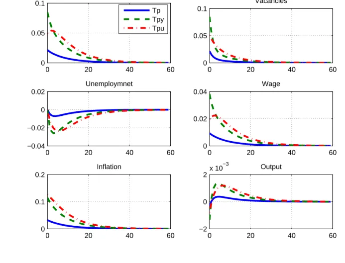
Once again strict inflation targeting tends to destabilize labour market variables and to smooth inflation dynamic. On the opposite side stands the Taylor rule. And again targeting unemployment along with inflation helps to stabilize both inflation and labor market variables.
4
Welfare Analysis
As specified above the optimal policy problem in this context is solved by assuming that the monetary authority maximizes households welfare subject to the competitive equilibrium conditions and the monetary policy rule represented by (25). Specifically I search for parametrization of interest rate rules that satisfy the following 3 conditions: a) they are simple since they involve only observable variables, b) they guarantee uniqueness of the rational expectation equilibrium, c) they
maximize the expected life-time utility of the representative agent. To this purpose I identify a class of rule based on the condition a), then I identify a grid search of parameters based on criterion b),finally I search for the parametrization that maximize agents’ utility.
Some observations on the computation of welfare in this context are in order. First, one cannot safely rely on standard first order approximation methods to compare the relative welfare associated to each monetary policy arrangement. Indeed in an economy with a distorted steady state stochastic volatility affects bothfirst and second moments of those variables that are critical for welfare. Since in a first order approximation of the model’s solution the expected value of a variable coincides with its non-stochastic steady state, the effects of volatility on the variables’ mean values is by construction neglected. Hence policy arrangements can be correctly ranked only by resorting to a higher order approximation of the policy functions.12 Additionally one needs to focus on the conditional expected discounted utility of the representative agent. This allows to account for the transitional effects from the deterministic to the different stochastic steady states respectively implied by each alternative policy rule.13Define Ωas the fraction of household’s consumption that would be needed to equate conditional welfare W0 under a generic interest rate
policy to the level of welfareWf0 implied by the optimal rule. HenceΩ should satisfy the following
equation: W0,Ω=E0 ( ∞ X t=0 βtU((1 +Ω)Ct) ) =Wf0
Under a given specification of utility one can solve for Ωand obtain:
Ω= expn³Wf0−W0
´
(1−β)o−1
4.1
Optimal Monetary Policy Rule
I simulate the model economy under the two sources of aggregate uncertainty, productivity and government consumption shocks. I then conduct two experiments. First, I compute welfare under different (ad hoc) specifications of the monetary policy rule. The rules are the following:
1 2See Kim and Kim (2003) for an analysis of the inaccuracy of welfare calculations based on log-linear
approxima-tions in dynamic open economies.
(i) Simple Taylor rule, withφπ = 1.5,φy = 0.5, φu =φr= 0;
(ii)Simple Taylor rule with smoothing, withφπ = 1.5 and φy = 0.5, φu= 0, φr= 0.9; (iii) Strict inflation targeting, φπ = 3, φy=φu =φr = 0;
(iv)Inflation + unemployment targeting, with φπ = 1.5,φu = 0.5,φy =φr= 0; (v) Strong inflation + unemployment targeting, withφπ = 3,φu = 0.5,φy = 0, φr = 0; (vi) Inflation + wage growth targeting,withφπ = 3,φu = 0,φy =φr = 0, φw = 0.5,where φw
indicates the parameter on wage growth.
Secondly, I search in the grid of parameters ©φπ, φy, φu, φrª for the rule which delivers the highest level of welfare, which is defined as the optimal policy rule.14
The choice of including unemployment as an independent argument comes from the consider-ation that most central banks face a trade-off between inflation and unemployment stabilization. In this respect it is natural to ask whether the price stability objective so much professed lately can be really considered the optimal policy.
Table (2) summarizes the findings and reports the values of the parameter which maximize conditional welfare, as well as the welfare loss Ω (relative to the optimal policy) of alternative simple rules.
Results are as follows. First, among the simple rules targeting unemployment along with inflation is the optimal rule. The reason for this is simple. In standard new-keynesian models mark-up constancy, hence marginal cost stabilization allows to achieve also inflation stabilization. On the contrary in a model with matching frictions the dynamic of marginal cost also depend on the evolution of unemployment. In this context it is not possible to obtain inflation stabilization without targeting unemployment as well. By smoothing unemploymentfluctuations the monetary authority can reduce the congestion effect typically associated with matching frictions thereby maximizing welfare. In addition it must be noticed that optimality requires targeting unemployment along with an aggressive inflation stabilization.
Secondly, targeting output along with inflation is welfare detrimental. This result is consis-tent with the one obtained by Schmitt-Grohe and Uribe (2004) in a model economy with capital
1 4The search is made over the following ranges: [0,4]forφ
π,[0,0.5]forφu,[0,1] forφy.I also compare rules with
interest rate smoothing (φr= 0.9)to rules without smoothing (φr= 0). It is judged as admissible a combination of
accumulation and frictionless labor markets. In the context of the present paper the reason for which targeting output gaps is welfare detrimental is due to the fact that the policy maker aims at targeting only gaps which signal an inefficiency. In this case since the friction affects only the labor market targeting the unemployment gap provides the right target.
Third interest smoothing is always welfare enhancing. Also this result is consistent with the one obtained by Schmitt-Grohe and Uribe (2004) and can be explained with the fact that interest rate smoothing allows to protract the stabilization effects of the monetary policy targets.
Finally targeting wage growth is welfare detrimental. The latter result can be explained again by the fact that the marginal cost in this model is not equalized to real wages but depends also on the evolution of unemployment, hence stabilizing wage growth is not sufficient to stabilize marginal cost and inflation. On the contrary by targeting unemployment the policy maker is able to close the whole marginal cost gap hence the whole inflation gap.
4.2
Responding to Unemployment and Wages
To further investigate whether the response to unemployment in a Taylor rule helps to increase welfare, figure (3) reports the effects on conditional welfare of varying both the inflation and the unemployment coefficients on the monetary policy rule. It shows that increasing the weight on unemployment significantly improves welfare and that the maximum utility is reached under strong inflation targeting together with unemployment targeting.
This result is in contrast with optimal policy prescriptions obtained by the vast majority of papers which employed a new keynesian framework (whose relevant frictions are price rigidity and monopolistic competition). As stressed in Blanchard and Gali’ (2005) the new keynesian framework is characterized by a “divine coincidence” for which stabilizing inflation implies invariably output stabilization. They showed that by introducing labor market rigidities in the form of exogenously imposed wage rigidities allows to beak this divine coincidence and to revive the unemployment inflation trade-off. In the context of the present paper the sole presence of search frictions produce an inefficiently low level of employment and this introduces a trade-off between inflation and em-ployment/output stabilization. In presence of such trade-offthe monetary authority should strike a balance between reducing the cost of adjusting prices and increasing employment.
policy rule for both inflation and real wage growth15. Again we observe that targeting wage growth does not improve welfare for any value of the parameter on inflation. The result is confirmed also under a high degree of real wage stickiness (λ = 0.9), see (5). Notice that this seems in contrast with results previously obtained in the literature. More specifically, Erceg, Henderson and Levin (2000), Schmitt-Grohe and Uribe (2006) and Canzoneri, Cumby and Diba (2005) find that it is optimal to target wage inflation. The difference between this paper result and the previous ones can be explained by the following considerations. First, previous authors were considering nominal wage growth targeting (wage inflation targeting) while here I consider real wage growth. Secondly, previous literature had introduced labor market frictions only in then form of nominal wage rigidity a’ la Calvo while I also consider a non-walrasian labor market.
5
Conclusion
This paper derives a constrained Ramsey policy in a model with monopolistic competition and sticky prices, matching frictions and real wage rigidity in the labour market. Further it compares welfare under different monetary policy rules. It concludes that the introduction of labor market rigidities implies that the optimal rule must deviate from strict inflation targeting. This is so since the matching frictions add a congestion externality due to which the number of unemployed in the market and their bargaining power reduces the probability of forming matches. The marginal cost in this case depends also on the evolution of unemployment. This induces a typical unemploy-ment/inflation trade-offthat calls for unemployment targeting along with inflation targeting.
1 5
It is worth noticing that the determinacy region under wage growth targeting shrinks compared to the case of unemployment targeting. It is not surprising to observe indeterminacy for some parameters’ regions in models with matching frictions. Indeed as it has been observed in Krause and Lubik (2005) and Hashimzade and Ortigueira (2005) the presence of search externality tends to produce indeterminacy.
References
[1] Andolfatto, David (1996). “Business Cycles and Labor Market Search”. American Economic Review 86, 112-132.
[2] Andrés, Javier, David López-Salido and Javier Vallés (2001). “Money in a Estimated Business Cycle Model of the Euro Area”. Banco de España, WP 0121.
[3] Angeloni, Ignazio, and Luca Dedola. (1998) “From the ERM to the EMU: New Evidence on Convergence in the Euro Area”. ECB w.p.
[4] Basu, Susanto and John Fernald (1997). “Returns to Scale in U.S. Production: Estimates and Implications”.Journal of Political Economy, vol. 105-2, pages 249-83.
[5] Blanchard, Olivier and Paul Diamond (1991). “The Aggregate Matching Function”. NBER Working Papers 3175.
[6] Blanchard, Olivier, and Jordi Gali’, 2006. “Real Wage Rigidities and the New Keynesian Model”, forthcomingJournal of Money, Credit and Banking.
[7] Canzoneri, Matthew, R. Cumby and B. Diba, (2005), “Price and Wage Inflation Targeting: Variations on a Theme by Erceg, Henderson and Levin”. Mimeo.
[8] Christofell, Kai and Tobias Linzert, 2005. “ The Role of Real Wage Rigidity and Labor Market Flows for Unemployment and Inflation Dynamics”. Mimeo.
[9] Clarida, Richard, Jordi Gali, and Mark Gertler, (2000). “Monetary Policy Rules and Macro-economic Stability: Evidence and Some Theory”. Quarterly Journal of Economics, 115 (1), 147-180.
[10] Cole Harald L. and R. Rogerson, (1996). “Can the Mortensen-Pissarides matching model match the business cycle facts?”. StaffReport 224, Federal Reserve Bank of Minneapolis.
[11] Cooley, Thomas and Vincenzo Quadrini, 2004. “Investment and liquidation in renegotiation-proof contracts with moral hazard”.Journal of Monetary Economics, 51(4), 713-751.
[12] den Haan, Wouters, Gary Ramey, and James Watson, (2000). “Job Destruction and Propaga-tion of Shocks”.American Economic Review 90, 482-498.
[13] Erceg, Christopher J., Henderson, Dale W. and Andrew T. Levin, 2000. “Optimal monetary policy with staggered wage and price contracts”.Journal of Monetary Economics, 46(2), 281-313.
[14] Faia, Ester (2005), “Ramsey Monetary Policy with Capital Accumulation and Nominal Rigidi-ties”, forthcoming inMacroeconomic Dynamics.
[15] Faia, Ester and Tommaso Monacelli (2005). “Optimal Monetary Policy Rules with Credit
[16] Hashimzade, Nigar and Salvador Ortigueira, (2005). “Endogenous Business Cycles with Fric-tional Labour Markets”.Economic Journal.
[17] Hall, Robert (2003). “Wage Determination and Employment Fluctuations”. NBER W. P. #9967.
[18] Hosios, Arthur J, 1990. “On the Efficiency of Matching and Related Models of Search and Unemployment”.Review of Economic Studies, 57(2), 279-98.
[19] Merz, Monika (1995). “Search in the Labor Market and the Real Business Cycle”.Journal of Monetary Economics 36, 269-300.
[20] Mortensen, D. and C. Pissarides, (1999). “New Developments in Models of Search in the Labor Market”. In: Orley Ashenfelter and David Card (eds.): Handbook of Labor Economics.
[21] Kim J., K.S. Kim (2003). “Spurious Welfare Reversals in International Business Cycle Models”.
Journal of International Economics 60, 471-500.
[22] Kim J. and Andrew Levin (2004). “Conditional Welfare Comparisons of Monetary Policy Rules”. Mimeo.
[23] King Robert G. and Alexander L. Wolman, 1996. “Inflation Targeting in a St. Louis Model of the 21st Century”. NBER W. P. 5507.
[24] Kollmann Robert, (2003a). “Monetary Policy Rules in an Interdependent World”. CEPR DP 4012.
[25] Kollmann Robert, (2003b). “Welfare Maximizing Fiscal and Monetary Policy Rules”. Mimeo.
[26] Krause, Michael and Thomas Lubik, (2005). “The (Ir)relevance of Real Wage Rigidity in the New Keynesian Model with Search Frictions”. forthcoming inJournal of Monetary Economics.
[27] Krause, Michael and Thomas Lubik, (2004). “A Note on Instability and Indeterminacy in Search and Matching Models”. Mimeo.
[28] Nickell, Stephen, and Luca Nunziata. (2001) “Labour Market Institutions Database.”
[29] Perotti, Roberto (2004). “Estimating the Effects of Fiscal Policy in OECD Countries”. Mimeo.
[30] Rotemberg, Julio (1982). “Monopolistic Price Adjustment and Aggregate Output”.Review of Economics Studies, 44, 517-531.
[31] Ramsey, F. P. (1927). “A contribution to the Theory of Taxation”.Economic Journal, 37:47-61.
[32] Rotemberg, Julio and Michael Woodford (1997). “An Optimization-Based Econometric Model for the Evaluation of Monetary Policy”. NBER Macroeconomics Annual,12: 297-346.
[33] Schmitt-Grohe, Stephanie and Martin Uribe (2003). “Optimal, Simple, and Implementable Monetary and Fiscal Rules”. Mimeo.
[34] Schmitt-Grohe, Stephanie and Martin Uribe (2004a). “Solving Dynamic General Equilibrium Models Using a Second-Order Approximation to the Policy Function”. Journal of Economic Dynamics and Control 28, 645-858.
[35] Schmitt-Grohe, Stephanie and Martin Uribe (2004b). “Optimal Operational Monetary Policy in the Christiano-Eichenbaum-Evans Model of the U.S. Business Cycle ”. Mimeo.
[36] Schmitt-Grohe, Stephanie and Martin Uribe, (2005), “Optimal Inflation Stabilization in a Medium-Scale Macroeconomic Model”. Mimeo.
[37] Shimer, Robert (2003). “The Cyclical Behavior of Equilibrium Unemployment and Vacancies: Evidence and Theory”. forthcomingAmerican Economic Review.
[38] Smets,Frank and Raf Wouters, 2003. “An Estimated Dynamic Stochastic General Equilibrium Model of the Euro Area”.Journal of the European Economic Association, 1(5), 1123-1175.
[39] C. Walsh, (2003), “Labor Market Search and Monetary Shocks”. In: S. Altug, J. Chadha, and C. Nolan (eds.): Elements of Dynamic Macroeconomic Analysis, Cambridge University Press
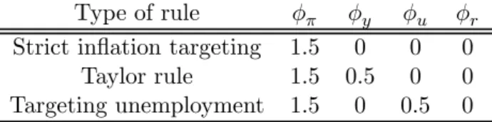
Table 1: Monetary policy rules considered for the impulse response analysis.
Type of rule φπ φy φu φr
Strict inflation targeting 1.5 0 0 0 Taylor rule 1.5 0.5 0 0 Targeting unemployment 1.5 0 0.5 0
Table 2: Welfare comparison of alternative monetary policy rules.
Rule % Loss relative to optimal rule
Taylor rule 2.9778
Taylor rule with smoothing 0.3420 Strict inflation targeting 0.0077 Inflation + unemployment targeting 0.0340 Strong Inflation + unemployment targeting 0
0 10 20 30 40 50 60 0 0.2 0.4 0.6 0.8
Labor market tightness
0 10 20 30 40 50 60 0 0.2 0.4 0.6 0.8 Vacancies 0 10 20 30 40 50 60 −0.3 −0.2 −0.1 0 0.1 Unemploymnet 0 10 20 30 40 50 60 0 0.1 0.2 0.3 0.4 Wage 0 10 20 30 40 50 60 −1.5 −1 −0.5 0 0.5 Inflation 0 10 20 30 40 50 60 0 0.5 1 1.5 Output Tp Tpy Tpu
Figure 1: Impulse responses to productivity shocks under the three rules described in table (1).
0 20 40 60 0
0.05 0.1
Labor market tightness
0 20 40 60 0 0.05 0.1 Vacancies 0 20 40 60 −0.04 −0.02 0 0.02 Unemploymnet 0 20 40 60 0 0.02 0.04 Wage 0 20 40 60 0 0.1 0.2 Inflation 0 20 40 60 −2 0 2x 10 −3 Output Tp Tpy Tpu
Figure 2: Impulse responses to government expenditure shocks under the three rules described in table (1).
0 0.05 0.1 0.15 0.2 0.25 0.3 0.35 0.4 0.45 0.5 1.5 2 2.5 3 3.5 4 −0.4 −0.39 −0.38 −0.37 −0.36 −0.35 −0.34 −0.33 −0.32 −0.31 Response to Unemployment Effect on Welfare of Varying the Response to Inflation and Unemployment
Response to Inflation
Conditional Welfare
0 0.1 0.2 0.3 0.4 1.5 2 2.5 3 −0.3 −0.25 −0.2 −0.15 −0.1
Response to Wage Growth Effect on Welfare of Varying the Response to Inflation and Wage Growth
Response to Inflation
Conditional Welfare
0 0.1 0.2 0.3 0.4 1.5 2 2.5 3 −0.3 −0.25 −0.2 −0.15 −0.1
Response to Wage Growth Effect on Welfare of Varying the Response to Inflation and Wage Growth (high wage rigidity)
Response to Inflation
Conditional Welfare
European Central Bank Working Paper Series
For a complete list of Working Papers published by the ECB, please visit the ECB’s website (http://www.ecb.int)
665 “The euro as invoicing currency in international trade” by A. Kamps, August 2006. 666 “Quantifying the impact of structural reforms” by E. Ernst, G. Gong, W. Semmler and
L. Bukeviciute, August 2006.
667 “The behaviour of the real exchange rate: evidence from regression quantiles” by K. Nikolaou, August 2006.
668 “Declining valuations and equilibrium bidding in central bank refinancing operations” by C. Ewerhart, N. Cassola and N. Valla, August 2006.
669 “Regular adjustment: theory and evidence” by J. D. Konieczny and F. Rumler, August 2006. 670 “The importance of being mature: the effect of demographic maturation on global per-capita
GDP” by R. Gómez and P. Hernández de Cos, August 2006.
671 “Business cycle synchronisation in East Asia” by F. Moneta and R. Rüffer, August 2006.
672 “Understanding inflation persistence: a comparison of different models” by H. Dixon and E. Kara, September 2006.
673 “Optimal monetary policy in the generalized Taylor economy” by E. Kara, September 2006. 674 “A quasi maximum likelihood approach for large approximate dynamic factor models” by C. Doz,
D. Giannone and L. Reichlin, September 2006.
675 “Expansionary fiscal consolidations in Europe: new evidence” by A. Afonso, September 2006. 676 “The distribution of contract durations across firms: a unified framework for understanding and
comparing dynamic wage and price setting models” by H. Dixon, September 2006.
677 “What drives EU banks’ stock returns? Bank-level evidence using the dynamic dividend-discount model” by O. Castrén, T. Fitzpatrick and M. Sydow, September 2006.
678 “The geography of international portfolio flows, international CAPM and the role of monetary policy frameworks” by R. A. De Santis, September 2006.
679 “Monetary policy in the media” by H. Berger, M. Ehrmann and M. Fratzscher, September 2006. 680 “Comparing alternative predictors based on large-panel factor models” by A. D’Agostino and
682 “Is reversion to PPP in euro exchange rates non-linear?” by B. Schnatz, October 2006. 683 “Financial integration of new EU Member States” by L. Cappiello, B. Gérard, A. Kadareja and
S. Manganelli, October 2006.
684 “Inflation dynamics and regime shifts” by J. Lendvai, October 2006.
685 “Home bias in global bond and equity markets: the role of real exchange rate volatility” by M. Fidora, M. Fratzscher and C. Thimann, October 2006
686 “Stale information, shocks and volatility” by R. Gropp and A. Kadareja, October 2006. 687 “Credit growth in Central and Eastern Europe: new (over)shooting stars?”
by B. Égert, P. Backé and T. Zumer, October 2006.
688 “Determinants of workers’ remittances: evidence from the European Neighbouring Region” by I. Schiopu and N. Siegfried, October 2006.
689 “The effect of financial development on the investment-cash flow relationship: cross-country evidence from Europe” by B. Becker and J. Sivadasan, October 2006.
690 “Optimal simple monetary policy rules and non-atomistic wage setters in a New-Keynesian framework” by S. Gnocchi, October 2006.
691 “The yield curve as a predictor and emerging economies” by A. Mehl, November 2006. 692 “Bayesian inference in cointegrated VAR models: with applications to the demand for
euro area M3” by A. Warne, November 2006.
693 “Evaluating China’s integration in world trade with a gravity model based benchmark” by M. Bussière and B. Schnatz, November 2006.
694 “Optimal currency shares in international reserves: the impact of the euro and the prospects for the dollar” by E. Papaioannou, R. Portes and G. Siourounis, November 2006.
695 “Geography or skills: What explains Fed watchers’ forecast accuracy of US monetary policy?” by H. Berger, M. Ehrmann and M. Fratzscher, November 2006.
696 “What is global excess liquidity, and does it matter?” by R. Rüffer and L. Stracca, November 2006. 697 “How wages change: micro evidence from the International Wage Flexibility Project”
by W. T. Dickens, L. Götte, E. L. Groshen, S. Holden, J. Messina, M. E. Schweitzer, J. Turunen, and M. E. Ward, November 2006.