Working Paper No. 20/12
Decomposing Differences in Labour Force Status
between Indigenous and Non-Indigenous Australians
between Indigenous and Non-Indigenous Australians*
Guyonne Kalb
†, Trinh Le
†, Boyd Hunter
‡and Felix Leung
†† Melbourne Institute of Applied Economic and Social Research,
The University of Melbourne
‡ Centre for Aboriginal Economic Policy Research,
The Australian National University
Melbourne Institute Working Paper No. 20/12
ISSN 1328-4991 (Print)
ISSN 1447-5863 (Online)
ISBN 978-0-7340-4280-4
August 2012
* This paper is based on research commissioned by the Australian Government Department of Education, Employment and Workplace Relations (DEEWR) under the Social Policy Research Services Agreement (2010-2012) with the Melbourne Institute of Applied Economic and Social Research. The paper uses the confidentialised unit record file from the Department of Families, Housing, Community Services and Indigenous Affairs’ (FaHCSIA) Household, Income and Labour Dynamics in Australia Survey, which is managed by the Melbourne Institute of Applied Economic and Social Research. The views expressed in this paper are those of the authors alone and do not represent the views of DEEWR, FaHCSIA, the Commonwealth Government or the Melbourne Institute. For their helpful comments and suggestions, we would like to thank DEEWR staff, John Haisken-DeNew and seminar attendants at Melbourne Institute, DEEWR and the 2012 Econometric Society Australasian Meeting. Any remaining errors are our own.
Melbourne Institute of Applied Economic and Social Research The University of Melbourne
Victoria 3010 Australia
Telephone (03) 8344 2100
Fax (03) 8344 2111
Email [email protected]
Abstract
Despite several policy efforts to promote economic participation by Indigenous Australians, they continue to have low participation rates compared to non-Indigenous Australians. This study decomposes the gap in labour market attachment between Indigenous and non-Indigenous Australians in non-remote areas, combining two separate data sources in a novel way to obtain access to richer information than was previously possible. It shows that among women at least two thirds of the gap can be attributed to differences in the observed characteristics between the two populations. For men, the differences in observed characteristics of the two populations can account for 36 to 47 percent of the gap. A detailed decomposition shows that lower education, worse health, and larger families (particularly for women) explain the lower labour market attachment of Indigenous Australians to a substantial extent. Compared with previous studies, this study is able to explain a larger proportion of the gap in employment between Indigenous and non-Indigenous people due to being able to include a larger set of explanatory variables.
JEL classification: J15
1. Introduction
Australia is one of the few developed countries that have a sizeable, disadvantaged indigenous minority. This minority, collectively known as Indigenous Australians, includes people of Aboriginal and/or Torres Strait Islander origins and makes up around 2.5 percent of the country’s population. Various data sources show that Indigenous Australians continue to suffer considerable disadvantage compared to other Australians. For example, life expectancy for male Indigenous Australians is about 11.5 years lower than for other male Australians and for female Indigenous Australians it is 9.7 years lower (Australian Bureau of Statistics (ABS), 2009). In 2006, Year 12 completion for Indigenous Australians aged 20-24 was 45.3 percent, compared to 86.3 percent for non-Indigenous counterparts. While 72 percent of the non-Indigenous working-age population were in employment in 2006, only 48 percent of Indigenous Australians were employed (FaHCSIA, 2009). The Council of Australian Governments has clear focus on this issue with an explicit ‘Closing the gap’ target of halving the Indigenous gap in employment outcome by 2018 (Steering Committee for the Review of Government Service Provision, 2010).
Since the early days of colonisation, Indigenous people have had limited participation in the mainstream labour market compared to other Australians. Certainly the measured employment gap has been large since Indigenous Australians were comprehensively included in the national official population statistics in 1971. There have been numerous public policy efforts to redress the gaps, including the Aboriginal Employment Development Policy introduced in 1987 by the Hawke government which committed to ‘statistical equality’ in employment, income and educational status between Aboriginal and other Australians by the year 2000, the Howard government’s notion of ‘practical reconciliation’ introduced in 1998, and most recently the Rudd government’s ‘Closing the gap’ strategy introduced in 2008 (Altman, Biddle and Hunter, 2008).
At the heart of the ‘Closing the gap’ strategy is the target of halving the Indigenous gap in employment outcome by 2018. This is an ambitious target, given the evidence that employment rates for the two populations would diverge while labour force participation rates would take over a century to converge if the trends for the period 1971-2006 were to persist (Altman, Biddle and Hunter, 2008).1
Policy debates and developments on closing the Indigenous gap in employment would benefit from a better understanding of the factors that affect labour market participation by Indigenous versus non-Indigenous Australians. This study seeks to broaden the evidence base by decomposing the gap in labour market attachment between the two populations. The study aims to provide further insights on the extent to which the gaps in labour market outcomes between Indigenous and non-Indigenous Australians can be explained by differences in observed characteristics of the two populations and on the extent to which they can be attributed to differences in the effects that observed characteristics have on labour market outcomes.
Since Indigenous Australians are only a small share of the country’s population, no general sample survey contains enough Indigenous respondents for detailed regression analysis. The Census of Population and Housing has a size advantage, but contains few individual and family characteristics. This study avoids these data limitations by drawing on different surveys for Indigenous and non-Indigenous populations. In particular, analyses of Indigenous people are based on the 2008 National Aboriginal and Torres Strait Islander Social Survey (NATSISS), which is the most recent cross-sectional data set focussing on the Indigenous population. Non-Indigenous Australians are drawn from a general household survey, the 2008 wave of the Household, Income and Labour Dynamics Australia (HILDA).2 The study focuses on non-remote areas, as HILDA’s reference population excludes remote areas (Summerfield et al., 2011), so we only observe respondents in remote regions if they moved there from a non-remote region during the survey.3 There are also other reasons to exclude
remote regions, as the labour markets in remote areas are characterised by a much higher prevalence of the ‘customary’ sector4 (Altman, Buchanan and Biddle, 2006) and of government interventions such as the Community Development Employment Projects
2 We use the Confidentialised Unit Record Files (CURFs) for all unit-record data.
3 In both surveys, remoteness is defined using the Accessibility/Remoteness Index of Australia (ARIA), which measures the remoteness of a point based on the physical road distance to the nearest urban centre. Remote areas are those scoring a grade 4 (remote: very restricted accessibility of goods, services and opportunities for social interaction, e.g. Alice Springs and Mount Isa) or 5 (very remote: very little accessibility of goods, services and opportunities for social interaction, e.g. Warburton and Balgo). These areas make up 86 percent of Australia’s landmass, but only 6 percent of its population (Department of Health and Aged Care, 2001). 4 The ‘customary’ sector includes activities such as hunting, fishing and gathering, production of art and crafts,
(CDEP) than in non-remote areas. Moreover, relatively few non-Indigenous people live in remote areas.5
Several studies have decomposed the gap in labour force participation between Indigenous and non-Indigenous Australians. The current study makes three contributions to the literature. First, while most previous decomposition studies only distinguish two labour force states (either whether employed or participating in the labour force), we distinguish four states: not in the labour force, unemployed, part-time employed, and full-time employed. Second, by combining the NATSISS and HILDA data we are able to control for a wider range of factors than previous studies have used. Third, we use new econometric methods that not only decompose the gap in labour market attachment into explained and unexplained components, but also further decompose the explained gap into contributions by each characteristic. In particular, the gap in labour market attachment between the two populations is decomposed using the Blinder (1973)-Oaxaca (1973) technique which has been generalised to non-linear models by Bauer and Sinning (2008), while detailed decomposition is based on the method proposed by Powers, Yoshioka and Yun (2011).
The rest of the study proceeds as follows. Section 2 provides background on Indigenous Australians’ labour market outcomes and reviews the literature on their labour market disadvantages. The methods and data are respectively described in Sections 3 and 4. Section 5 reports the regression results on labour force status of each population while Section 6 decomposes the gap in labour market attachment between the two populations. Section 7 summarises and concludes.
2. Brief literature review
2.1. Indigenous Australians’ labour market outcomes
Indigenous Australians’ labour market outcomes are characterised by high non-participation, unemployment and part-time employment. According to Census 2006 (see Kalb, Le and Leung, 2012: Table 4), among Indigenous Australians aged between 15 and 64, 44 percent were out of the labour force, 9 percent were unemployed while 40 percent of employed individuals worked less than 35 hours a week. The corresponding figures for non-Indigenous Australians were 25, 4 and 31 percent respectively. While less than a third of non-Indigenous
5 According to Census 2006, 1.8 percent of the non-Indigenous population live in remote areas, compared to 24 percent of the Indigenous population.
people had a weekly income of less than $400, almost 60 percent of Indigenous people were in this bracket.
Indigenous Australians are more likely to be employed in the public sector than other Australians. In addition, Indigenous employment is concentrated in just a few industries such as agriculture, and health and community services (Norris, 2001; Daly, 1995; Taylor, 1993). Movement between labour force states is also frequent among Indigenous Australians. Data from the Indigenous Job Seeker Survey reveal that Indigenous employment can be quite unstable with over 50 percent of currently full-time employed respondents becoming unemployed 15 months later (Gray and Hunter, 2005).
In 1977, a government employment programme known as CDEP was introduced to curb unemployment among Indigenous Australians in remote communities where employment opportunities were limited. In official statistics, CDEP work is often categorised as being employed, but it can just as easily be classified as unemployment with many commentators labelling it rather loosely as an Indigenous ‘work-for-the-dole’ scheme. The role of CDEP in improving other outcomes among Indigenous Australians has often been questioned (for example, Hunter, 2009).6
2.2. Decomposition studies on Indigenous Australians’ labour market disadvantages
One of the earlier studies exploring the income differences between Indigenous and non-Indigenous Australians is by Daly (1992). Applying the Blinder-Oaxaca decomposition method on Census 1986 data, the study finds that for Indigenous males 70 percent of the gap in income could be attributed to their lower levels of education and labour market experience and 30 percent to their lower returns to human capital and other attributes. For Indigenous females, the percentages were 44 and 56 respectively.
While it is straightforward to decompose differences in a continuous outcome like income, the income variable in Census data, which includes gross income from all sources (that is, including transfers and before taxes are deducted), is likely to understate the extent of the gap in labour market outcomes between Indigenous and non-Indigenous Australians. Analysing earnings, on the other hand, will exclude a large share of Indigenous Australians from the analysis as earnings are only observed for employed individuals.
6 Hunter and Gray (2012) show that CDEP participants have only slightly better outcomes for most measures than the unemployed and much worse than for the non-CDEP employed.
Using the 2001 Census, Hunter (2004) decomposes the gaps in employment rates between Indigenous and non-Indigenous Australians. The probability of employment of Indigenous Australians in the absence of ‘discrimination’ is calculated by imposing the same returns to the observed characteristics on Indigenous Australians as estimated for non-Indigenous Australians. By comparing the hypothetical and actual employment probabilities, Hunter (2004) shows that at most one third of the average employment differential can be explained by differences in observed characteristics between the two populations. Similar decompositions have been carried out by Miller (1989) and Daly (1993), who concluded about one fifth to a quarter of the gaps could be explained by differences in observed characteristics between the two populations. A common characteristic of studies that decompose the gaps in participation and employment outcomes between Indigenous and non-Indigenous Australians is that they only distinguish two labour force states, namely in versus out of the labour force or in versus out of employment. Moreover, these studies could only explain a small proportion of the gap in the outcome between Indigenous and non-Indigenous Australians. Most of the gap, therefore, is left to be attributed to other factors, such as unobserved differences, differences in behaviour, or, potentially, differences in treatment (discrimination).
3. Methods
3.1. Model of labour force status
Even though previous decomposition studies only distinguish two labour force states, studies on labour market participation of Indigenous Australians alone distinguish up to four labour force states: not in the labour force, unemployed and employed, occasionally further disaggregating employed into full-time and part-time or into mainstream labour market and CDEP. The current study distinguishes four labour force states: (1) not in the labour force, (2) unemployed, (3) part-time employed and (4) full-time employed. One point of departure from previous studies is that instead of modelling these categories as unranked outcomes using a multinomial logit model, we rank them in the order listed above and treat them as reflecting the extent of a person’s attachment to the labour market. That is, the underlying variable that these four outcomes measure is attachment to the labour market, where non-participation represents the lowest attachment and full-time employment represents the strongest attachment. To model labour market attachment, as manifested by those four ranked outcomes, we use the ordered logit method.
As Section 2.1 shows, not only are Indigenous Australians less likely to participate in the labour force, they are also more likely to be unemployed and to work part time. Therefore, a model that only distinguishes participants versus non-participants, or employed versus unemployed individuals will ignore the heterogeneity among labour force participants in each population. By allowing for four labour force states, the current model allows us to capture more detailed differences in participation and employment outcomes between the Indigenous and non-Indigenous Australians than a model distinguishing only two states.
3.2. Non-linear decomposition
After estimating the factors that affect the labour force status of Indigenous and non-Indigenous people, we use the Blinder (1973)-Oaxaca (1973) method to decompose the gap in labour market attachment between the two populations. For a linear regression, the standard Blinder-Oaxaca decomposition of the Indigenous/non-Indigenous gap in the mean value of labour market outcome Y can be expressed as:
(1)
where subscript A denotes the non-Indigenous population (the ‘majority’ group), subscript B the Indigenous population (the ‘disadvantaged’, or minority, group), is a row of mean values of the control variables and is a vector of coefficient estimates. The first term of equation (1) measures the gap due to differences in observed characteristics (the composition, or ‘explained’, gap). The second term measures the unexplained gap due to differences in coefficients, or returns to characteristics (the coefficient, or ‘unexplained’, gap).
Bauer and Sinning (2008) note that in non-linear models (such as logit), the conditional expectation | differs from the linear prediction . They thus re-write equation (1) to accommodate non-linear models:7
| | | | (2)
For an ordered logit model with four categories in the dependent variable (taking values of 0, 1, 2 and 3), the mean conditional expectation is:
7 Bauer and Sinning’s (2008) approach to decomposing non-linear outcomes has been used by Bauer, Göhlmann and Sinning (2007), Madden (2010) and Sinning (2011).
1
1 1
2
1 1 3 1 1
(3)
where j= A, B; Nj is the size of the group; and the s are threshold parameters that are
estimated along with the in the ordered logit model. The terms in parentheses are the probability of observing outcome value 1, 2 and 3 respectively.
A well-known issue with the Blinder-Oaxaca decomposition technique is the so-called index number problem; that is, the decomposition results vary with the choice of reference group. If the estimated coefficients (returns) for the non-Indigenous (Indigenous) population are used as the non-discriminatory basis, the decomposition involves addressing the question ‘What would the labour market attachment of the Indigenous (non-Indigenous) population be if they were to have the same set of coefficients as estimated for the non-Indigenous (Indigenous) population?’ Equation (1) refers to the case where non-Indigenous coefficients ( ) are used as the non-discriminatory basis.
It is argued that the ‘true’ non-discriminatory basis should lie somewhere between the Indigenous coefficients and the non-Indigenous coefficients:
(4)
where is a weighting matrix and is the identity matrix. The literature has proposed different weighting schemes to deal with the underlying index problem. Oaxaca (1973) proposed using either the coefficients for the majority group as the non-discriminatory basis (Ω = 1) or the coefficients for the disadvantaged group (Ω = 0). Reimers (1983) proposed using the mean coefficients (Ω = 0.5), while Cotton (1988) proposed weighting the coefficients by group size. By contrast, Neumark’s (1988) approach was to estimate a pooled model over both groups to obtain . In this study, we present the results for Ω = 0 and Ω = 1 (with a focus on the latter), as they represent the two extremes within which the results based on the other weighting schemes would lie.
3.3. Non-linear detailed decomposition
A detailed decomposition can be used to determine how much each characteristic contributes to explaining the gap. A linear detailed decomposition can be written as:
∑ (5)
∑ (6)
where is the composition gap (the first term in equation (1)), is the coefficient gap (the second term in equation (1)), and subscript k denotes the covariate.
In the non-linear case, since the conditional expectation differs from the linear prediction, the detailed decomposition of the two components into the contribution of each covariate would not add up to the total. Several alternative detailed non-linear decomposition methods have been proposed, but they are often onerous to execute. For example, Fairlie’s (2005) method involves creating a series of counterfactuals, where the coefficient of each covariate is switched to the reference group value in sequence. According to Fortin, Lemieux and Firpo (2011), this decomposition approach would be sensitive to the order of decomposition (i.e. be path dependent).
In this study, we adopt the detailed decomposition method proposed by Powers, Yoshioka and Yun (2011). The contribution of each covariate to the composition gap is:
∆ (7)
and to the coefficient gap:
∆ (8)
Powers, Yoshioka and Yun (2011) define the weights w as:
∆ ∑ (9)
∆ ∑ (10)
That is, the composition weights reflect the relative contribution of each covariate based on the magnitude of the difference in the mean value of the covariate, weighted by the effect of the covariate in group A. The coefficient weights reflect the relative contribution of each covariate based on the magnitude of the difference in the size of the effect, weighted by the
mean value of the covariate in group B. As equations (9) and (10) show, this decomposition method is simple and not path dependent.
The unexplained gap can be due to one or more factors, including omitted characteristics, unobservable characteristics, differences in behaviour or preferences, or discrimination. Given its complex interpretation, little can be learned by further decomposing the unexplained gap into contributions by each covariate. Thus, this study will only conduct a detailed decomposition of the explained gap.
4. Data
To date the only data source that contains sufficiently large numbers of both Indigenous and non-Indigenous Australians is the Australian Census of Population and Housing. However, despite its size advantage, the Census contains few of the individual and family characteristics that are typically used to analyse labour market behaviour. In this study, analyses of Indigenous people are based on NATSISS 2008 while non-Indigenous Australians are drawn from HILDA wave 8, which was collected around the same time. While using different surveys for different populations is less than ideal, the richness of information available from these surveys makes it possible for detailed models of labour force status to be estimated. In Kalb, Le and Leung (2012), we carefully checked the data from these two surveys against Census 2006 data (the Census closest in time to 2008) to make sure that the surveys were sufficiently representative and reliable.
4.1. NATSISS 2008
NATSISS 2008 is a multi-faceted social survey of Indigenous Australians, covering 13,307 persons. The survey was conducted in remote and non-remote areas in all States and Territories, collecting information on various topics including language and culture, social networks and support, health, education, housing, labour force status, and financial stress. A random selection of a number of Indigenous communities and outstations was made; and within these selected communities and outstations a random sample of dwellings was selected. Only Indigenous persons who were usual residents of private dwellings were
included in the survey.8 In non-community areas, dwellings were selected using a stratified multistage sample based on information at the mesh block level within Census Collection Districts. Within each household, a random sub-sample of usual residents of one or two adults (aged 15 years or over) and one or two children (aged 0-14 years) were selected for inclusion in the survey. Specifically, for selected households in discrete remote Indigenous communities and outstations, one Indigenous adult and one Indigenous child were selected and interviewed, whereas in non-remote and remote non-community areas up to two Indigenous adults and up to two Indigenous children per selected household were selected and interviewed. Detailed information was collected for these selected persons, while only a very limited number of demographic characteristics are collected on the other members in the households.
4.2. HILDA
HILDA is a longitudinal survey of Australian households which has been run annually since its implementation in 2001, covering approximately 13,000 individual respondents from more than 7,000 households living in private dwellings in non-remote areas. The survey collects information on a large number of individual and household characteristics, with standard demographic and labour market information collected in all waves.9 This study uses wave 8, since its timing matches that of NATSISS 2008.10 Unlike NATSISS 2008, which only collected information from selected members of sampled households, HILDA interviews all individuals in such households.
4.3. Descriptive statistics
The restricted geographic scope of the HILDA survey and other differences in survey design mean that it is necessary to exclude remote resident from the analysis. Our analytical samples include all residents of non-remote areas aged 15-64 (to cover the working-age population),
8 Some Collection Districts and Indigenous communities in remote and very remote areas with a small number of Indigenous households were excluded from the sampling frame. As a result, NATSISS 2008 has a higher level of under-coverage compared to other ABS surveys. More detailed information about the survey is available from ABS (2010).
9 Detailed information on HILDA can be found on the website http://melbourneinstitute.com/hilda/. Although the Indigenous population is represented in the HILDA, they are not oversampled, making the number of observations for this group too small for separate analyses. For discussion of the design of the HILDA Survey see Wooden and Watson (2007).
10 NATSISS 2008 was conducted during August 2008 to April 2009, while HILDA wave 8 was during August to December 2008.
but exclude full-time students (who are arguably constrained in their labour supply choices). Note that the exclusion of remote areas means that the complicating effect of the CDEP scheme on the Indigenous analysis can be ignored.
Consistent with Census data, NATSISS and HILDA 2008 show a large gap in labour force participation between Indigenous and non-Indigenous Australians (see Table 1). The gender gap in labour force status is larger among Indigenous people. While 80 percent of Indigenous men in non-remote areas participate in the labour force, only 57 percent of Indigenous women do. The corresponding figures for non-Indigenous people are 87 percent and 75 percent respectively. Among labour force participants, non-Indigenous Australians are much more likely to work full time and less likely to be unemployed than Indigenous Australians. Compared with non-Indigenous people, Indigenous people are less likely to have a partner, or to have completed Year 12 or a university degree. Indigenous people are more likely to live in households with more children, smoke or report bad health. Indigenous people are on average around five years younger than non-Indigenous counterparts.
A number of additional characteristics are available for Indigenous Australians only. We use these in the analysis of labour market outcomes for the Indigenous population, but not in the decomposition analysis. This shows that around half of all Indigenous men and women have a disability that limits their employment opportunities or daily activities. More than half of Indigenous men and women identify with their culture and attended at least one cultural event in the last year. About one in five Indigenous Australians report living in their homeland. Nine percent of men and ten percent of women was ever removed from their family. Indigenous men are much more likely to have been arrested in the past five years (22 percent) than Indigenous women (9 percent).
Table 1: Descriptive statistics by Indigenous status and gender
Indigenous Non-Indigenous Male Female Male Female
Dependent variables
Not in labour force 0.204 0.432 0.134 0.250
In labour force 0.796 0.568 0.866 0.750 Unemployed 0.127 0.090 0.029 0.026 Part-time employed 0.133 0.224 0.085 0.303 Full-time employed 0.536 0.254 0.752 0.420 Control variables Age 35.33 36.23 41.40 41.66 Partnered 0.522 0.489 0.642 0.656
Schooling (ref: Completed less than Year 10)
Completed Year 10 or 11 0.463 0.455 0.386 0.357
Completed Year 12 0.233 0.242 0.517 0.547
Post-school qualification (ref: None)
Has non-degree post-school qualification 0.303 0.313 0.384 0.28
Has degree 0.049 0.066 0.238 0.287
Region (ref: NSW major cities)
NSW Inner Regional 0.128 0.131 0.064 0.063
NSW Outer Regional 0.072 0.074 0.021 0.020
VIC Major Cities 0.044 0.043 0.193 0.191
VIC Inner/Outer Regional 0.041 0.041 0.058 0.060
QLD Major Cities 0.108 0.096 0.115 0.113 QLD Inner Regional 0.074 0.072 0.062 0.068 QLD Outer Regional 0.109 0.124 0.032 0.033 SA Non-remote 0.056 0.061 0.079 0.074 WA Major Cities 0.067 0.061 0.086 0.078 WA Inner/Outer Regional 0.036 0.041 0.024 0.019 TAS Non-remote 0.048 0.048 0.024 0.023
Balance of Australia - Non-remote 0.048 0.047 0.027 0.025
Has income from non-labour, non-government sources 0.094 0.171 0.526 0.527
Type of household (ref: Single occupant)
One family household 0.764 0.78 0.794 0.835
Mixed household 0.127 0.156 0.088 0.092
Number of children aged <=14 1.060 1.331 0.535 0.597
Health status (ref: Very good/ excellent health)
Good health 0.321 0.351 0.375 0.369
Fair health 0.148 0.178 0.127 0.117
Poor health 0.087 0.071 0.027 0.031
Daily smoker 0.489 0.470 0.211 0.165
Additional variables for Indigenous population only
Respondent has a disability 0.502 0.510
Speaks an Indigenous language well 0.085 0.078
Cultural identification 0.586 0.570
Lives in homelands 0.209 0.178
Attended cultural events in last 12 months 0.510 0.615
Lacks contact (less than once a month) 0.073 0.062
Ever removed from natural family 0.090 0.098
Arrested by police in past 5 years 0.221 0.088
Number of observations 1,815 2,421 3,687 4,120
Sources: NATSISS 2008 (Indigenous), HILDA wave 8 (non-Indigenous)
Notes: Entries are means, weighted by sampling weights. Samples include all individuals aged 15-64, excluding full-time students and residents of remote areas.
5. Regression results
This section reports the estimation results on labour force status of Indigenous people and non-Indigenous people using an ordered logit model. Since the logit coefficients, which are log odds ratios, do not have immediately intuitive interpretation, we will report the marginal effects for the ‘average’ person (i.e. an hypothetical individual with all characteristics set at the mean values), which give the change in the predicted probability of an outcome resulting from an increase of one unit in the relevant variable, holding the other variables at their respective means. The marginal effects of dummy variables are calculated as the change in predicted probability when moving from a value 0 to 1, while corresponding dummy variables for multi-categorical variables are also set to zero.11 There is a set of marginal effects for each outcome of the dependent variable. To keep the number of tables in this section manageable, we only report the marginal effects for the two highest outcomes: part-time employment and full-part-time employment. We have left out the marginal effects for the 12 regional dummy variables, which were mostly small and insignificant.12
Standard errors are adjusted to allow for ‘clustering’ of observations in the same household. This adjustment, which corrects for the possible dependence of individuals in the same household, is also necessary to improve the comparability of results from NATSISS and HILDA since the entire household is interviewed for HILDA while at most two adults from each household are interviewed for NATSISS.
5.1. Indigenous population
5.1.1 The benchmark specification
We first present the marginal effects for our benchmark specification estimated separately for Indigenous men and women in Table 2. This is the central model to be analysed in this paper. Given the large difference in labour force states between the two genders observed in Table 1, different factors are likely to affect the labour force status of men and women or the same factors may affect the labour force status of men and women to a different extent.
11 For example, the marginal effect for ‘good health’ is evaluated when changing health status from ‘very good/excellent health’ (the reference category) to ‘good health’, while holding ‘fair health’ and ‘poor health’ at zero.
12 The marginal effect on the lowest outcome (not in labour force) always has the opposite sign to that of the highest outcome (full-time employment). Since the outcomes are ordered, the marginal effects of the two middle outcomes (unemployment and part-time employment) fall between those of the lowest and highest outcomes, and together they add to zero.
Table 2: Marginal effects on the probabilities of employment by gender for Indigenous Australians, the benchmark specification
Male Female
Control variable Part-time Full-time Part-time Full-time
Age (effects of a 10-year increase) 0.003** -0.011*** 0.004*** 0.013***
Partnered -0.063*** 0.291*** 0.005 0.019
Schooling (ref: Completed less than Year 10)
Completed Year 10 or 11 -0.030*** 0.167*** 0.054*** 0.108***
Completed Year 12 -0.053*** 0.241*** 0.058*** 0.244***
Post-school qualification (ref: None)
Has non-degree post-school qualification -0.034*** 0.133*** 0.033*** 0.156***
Has degree -0.051 0.184** 0.029* 0.200***
Has income from non-labour, non-govt sources -0.008 0.031 0.003 0.013
Log equivalised income of other hh. members 0.001 -0.004 0.001 0.004
Type of household (ref: Single occupant)
One family household -0.001 0.006 0.016 0.046
Mixed household -0.010 0.038 0.000 0.001
Number of children aged <=14 0.012*** -0.050*** -0.028*** -0.098***
Health status (ref: Very good/ excellent health)
Good health 0.020* -0.067* -0.014* -0.075*** Fair health 0.047*** -0.193*** -0.026** -0.105*** Poor health -0.011 -0.551*** -0.093** -0.195*** Daily smoker 0.025*** -0.106*** -0.017** -0.057** Number of observations 1,815 2,421 Pseudo R-squared 0.152 0.141
Notes: Standard errors are adjusted to allow for ‘clustering’ due to multiple observations in the same household. *significant at 10%, **significant at 5%, ***significant at 1%. Twelve geographic dummies are included in the regressions but are not reported here.
The results show that labour market attachment is first increasing and then decreasing with age.13 For a man with average sample characteristics, the effect of being 10 years older is to increase the probability of part-time employment by 0.3 percentage points and decrease the probability of full-time employment by 1.1 percentage points. For women, the corresponding marginal effects are increases of 0.4 and 1.3 percentage points respectively.
While having a partner is associated with a 29 percentage point increase in full-time employment for men, its effect for women is almost zero and insignificant. The strong association between partnering status and employment status for men is because the characteristics that make a man attractive in the labour market, such as age, education, health,
13 Age enters the regression in both linear and quadratic terms. The marginal effects of age are computed as 2 where is the marginal effect for the linear term, is the marginal effect for the quadratic term, and is the mean age of individuals in the sample. The reported marginal effects of age are for a change of 10 years, as the effects of a one-year change in age are very small.
as well as unobserved factors like intelligence and drive, are also likely to make him attractive in the marriage market. While partnered women possess strong productivity characteristics, they have greater financial security through an employed partner and usually a higher domestic work burden, as men still tend to be the breadwinner and women take greater responsibility for the homemaking. Thus there are two counteracting effects on the probability of being in paid employment for partnered women. As a result, the observed link between partnering status and employment status is weak for women.
Education increases the probability of full-time employment and decreases the probability of part-time employment for men. For women, the effect is positive for both types of employment, and substantially larger for full-time employment. Men who have completed Year 12 are 24 percentage points more likely to be full-time employed (and 5.3 percentage points less likely to be part-time employed) than men who left school before Year 10, while a tertiary degree raises the probability of full-time employment by 18 percentage points (and has a small and insignificant effect on the probability of part-time employment) over those without post-school qualifications. For women the corresponding marginal effects are increases of 24 (5.8) and 20 (2.9) percentage points respectively. The different effects that education has on the two genders are likely to work through the effects of partnership. While partnered women are more likely to substitute domestic work for market work and therefore tend to have a preference for part-time employment, partnered men have a stronger tendency to increase work effort as the main breadwinner of the family.
Whether the individual has income from non-labour, non-government sources has no effect on labour force status and neither does the log of equivalised income of other household members.14 This could be because while income from other household members reduces the need for an individual to participate in the labour market, those who have good earnings capacity are also more likely to live with others who have good earnings capacity (i.e. the assortative mating phenomenon), and the ‘net’ effect of income seems to be zero.
Household type also has no effect on the labour force status of Indigenous Australians. The only significant household structure effect is that the presence of each child reduces the male adult’s probability of full-time employment by 5.0 percentage points and increases his
14 The modified OECD equivalence scale, which is commonly used in Australian studies (for example, see ABS, 2005), is adopted. This scale gives a weight of 1 to the first adult in the household, 0.5 to each additional adult, and 0.3 to each child. A value of 0 is assigned to the logarithm of non-positive equivalised income.
time employment probability by 1.2 percentage points. For women, the presence of each child reduces the probability of full-time employment by 9.8 percentage points and part-time employment by 2.8 percentage points.
Health has significant effects on employment for both men and women, but the effects are much larger for men, partly due to higher employment rates among men. For example, while poor health reduces the chance of full-time employment by 20 percentage points for women, the corresponding effect is 55 percentage points for men. A negative effect on full-time employment is also found for daily smoking.
A ‘basic’ specification including core control variables, similar to Gray and Hunter (1999), corresponding to the variables available in the Census data, is presented in Appendix Table 1.15 Compared to the more extended (‘benchmark’) specification above, which includes a wider range of variables, the pseudo R-squared value is considerably lower for men and women, indicating that less of the variation can be explained by this basic model.
There are no clear patterns with regard to the region in which men and women live, but most non-geographic variables in the basic specification are statistically significant at the 1% level and results for the set of variables that the two specifications have in common are similar. The marginal effects of completing school and obtaining post-school qualifications on being in full-time employment are higher in the basic specification than in the benchmark specification. The additional variables in the benchmark specification (such as health and the number of children) appear to have absorbed part of the effect attributed to education in the basic specification.16
5.1.2 Extended specification
Past studies have often found a strong link between cultural attachment and labour market participation among Indigenous Australians (e.g. Hunter and Gray, 2001; Stephens, 2010).
15 However, although Gray and Hunter (1999) control for ‘difficulty with speaking English’, we do not control for this, since only three Indigenous men and ten Indigenous women in our analytical samples report difficulty with speaking English.
16 We would have liked to include local characteristics such as the presence of employment services or schools, or unemployment rates in the region in which the individual resides. However, since at most 17 regions (by State and level of remoteness) can be distinguished in the NATSISS data, the level of disaggregation was too low to observe meaningful differences.
This section examines how cultural and other factors affect the labour force status among this population.17
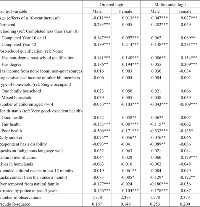
Table 3: Marginal effects on the probability of full-time employment for Indigenous Australians in an extended specification
Ordered logit Multinomial logit
Control variable Male Female Male Female
Age (effects of a 10-year increase) -0.011*** 0.013*** 0.047*** 0.027***
Partnered 0.293*** 0.005 0.282*** 0.049
Schooling (ref: Completed less than Year 10)
Completed Year 10 or 11 0.147*** 0.097*** 0.062 0.089**
Completed Year 12 0.189*** 0.214*** 0.148*** 0.231***
Post-school qualification (ref: None)
Has non-degree post-school qualification 0.141*** 0.148*** 0.086** 0.154***
Has degree 0.186** 0.194*** 0.055 0.209***
Has income from non-labour, non-govt sources 0.016 0.003 0.030 -0.034
Log equivalised income of other hh. members -0.006 0.004 -0.004 -0.002
Type of household (ref: Single occupant)
One family household 0.023 0.050 0.021 0.066
Mixed household 0.039 0.005 0.048 0.059
Number of children aged <=14 -0.053*** -0.103*** -0.043*** -0.109***
Health status (ref: Very good/ excellent health)
Good health -0.052 -0.058** -0.067* 0.007
Fair health -0.153*** -0.087*** -0.115** -0.062
Poor health -0.506*** -0.171*** -0.532*** -0.125*
Daily smoker -0.075** -0.056** -0.076** -0.046
Respondent has a disability -0.093** -0.041 -0.089** -0.036
Speaks an Indigenous language well 0.032 -0.063 0.021 -0.044
Cultural identification -0.044 0.028 -0.060 0.129***
Lives in homelands -0.063 -0.016 -0.062 -0.048
Attended cultural events in last 12 months 0.019 0.061** 0.004 0.049
Lacks contact (less than once a month) -0.083 -0.085* -0.129* -0.122**
Ever removed from natural family -0.177*** -0.024 -0.180*** -0.056
Arrested by police in past 5 years -0.126*** -0.104*** -0.178*** -0.087
Number of observations 1,778 2,373 1,778 2,373
Pseudo R-squared 0.167 0.149 0.253 0.200
Notes: Standard errors are adjusted to allow for ‘clustering’ due to multiple observations in the same household. *significant at 10%, **significant at 5%, ***significant at 1%. Twelve geographic dummies are included in the regressions but are not reported here.
As reported in the first two columns of Table 3, neither proficiency in an Indigenous language nor cultural identification (defined as identification with a clan, tribal or language group) has a consistent significant impact on labour force status of Indigenous people. While
17 These cultural variables are unique to NATSI(H/S)S and mostly irrelevant to the non-Indigenous population. Therefore, they cannot be used in the decomposition between Indigenous and non-Indigenous populations.
attendance of cultural events in the past 12 months is associated with an increase by 6.1 percentage points in the probability of full-time employment for women, no significant effect is found for men. The most significant variables among this ‘extended’ set are being removed from family as a child and police arrest. Having been arrested in the last five years is associated with a decrease by 13 percentage points in full-time employment among men and 10 percentage points among women. Having been removed as a child is associated with a decrease by 18 percentage points in full-time employment among men. The effect is insignificant and small for women.
Compared with the benchmark specification, this further extended specification has better goodness of fit (see the pseudo R-squared) and the coefficients on the ‘benchmark’ variables only change slightly, suggesting that the effects that the extra controls have on the dependent variable are additional to those already captured by the standard socio-economic and demographic variables.18
Compared with previous studies, this study has found a somewhat weaker relationship between cultural factors and labour force status. In an alternative specification (also presented in Table 3), we use a multinomial logit model (i.e. the labour force states are not ranked), which has often been used in previous studies, including the same extended set of variables. Overall the marginal effects are broadly similar between the two specifications. Again none of the results on the cultural variables are consistent between men and women, or across the cultural variables in either specification. Few of the coefficients on these variables are significant. This lack of effect is perhaps not so surprising since outside of remote areas, the fact that someone lives in homelands does not imply poor labour market opportunities, and therefore does not necessarily have any significant adverse effects on labour market outcomes. Indigenous cultural factors are particularly important in remote areas where there is usually an underdeveloped labour market with limited employment opportunities and
18 In an earlier version of this study, Kalb, Le and Leung (2012) found erratic effects of alcohol use on labour force status. According to Chikritzhs and Liang (2012), the data on alcohol use in NATSISS 2008 understate the incidence of high-risk drinking by a factor of two for males and seven for females. Since NATSISS 2008 excludes residents of non-private dwellings (who are less likely to be employed and more likely to abuse alcohol), the association between alcohol abuse and the labour force status of Indigenous Australians may be understated. In addition, the results based on the 2004 National Aboriginal and Torres Strait Islander Health Survey (NATSIHS), which has more reliable data on alcohol use, show small negative effects from all levels of alcohol use (see Kalb, Le and Leung, 2012: Appendix Table 7), further suggesting that the estimated results on alcohol use based on NATSISS 2008 are likely to be driven by measurement error in the alcohol variable. Therefore, alcohol use has been excluded from the models.
hence the weaker observed relationship can easily be rationalised by the exclusion of such areas.
5.2. Non-Indigenous population
5.2.1 Non-Indigenous versus Indigenous
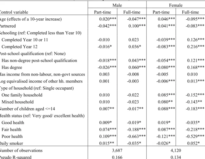
Table 4 reports the marginal effects on the probabilities of part-time and full-time employment for non-Indigenous Australians under the benchmark specification. The effects of education are weaker for non-Indigenous people than for Indigenous people, whereas number of children in the household and poor health show stronger effects for non-Indigenous Australians. For example, a university degree raises the probability of full-time employment by 6 percentage points for the reference non-Indigenous man, which is a third of the corresponding effect for the reference Indigenous man (18 percentage points, see Table 2).19 While poor health reduces the likelihood of full-time employment by 55 percentage points for the reference Indigenous man (Table 2), its corresponding effect on the reference non-Indigenous man is substantially higher at 66 percentage points. The larger effect of education and the smaller effect of poor health are likely to be due to the overall low level of full-time employment amongst Indigenous men compared to non-Indigenous men. Although daily smoking has a significant, negative effect on full-time employment of Indigenous men and women, its effect is positive for Indigenous women and seems smaller for non-Indigenous men than for non-Indigenous men. For non-non-Indigenous men and women, its effect on part-time employment is opposite to the effect on full-time employment.
5.2.2 Male versus Female
Large gender differences are also observed among non-Indigenous people. In contrast to the effects for the Indigenous population, education has a larger effect on women’s labour force status than on men’s. While Year 12 completion has little effect on non-Indigenous men’s employment, it adds 22 percentage points to the full-time employment probability among women. A tertiary degree makes a non-Indigenous woman 17 percentage points more likely to work full time than a woman without a post-school qualification, which is nearly three times the corresponding effect on men. A potential explanation for this difference in effects is that, in contrast to Indigenous men, non-Indigenous men are participating in the labour force
19 Caution should be exercised when comparing marginal effects across samples, as they are calculated based on the ‘reference’ person, which varies across samples. For example, the reference person in the Indigenous sample, who has the sample average age, is five year younger than that in the non-Indigenous sample (see Table 1. Their household income and number of household children are also different.
to a very large extent, and mostly full time, independent of the exact level of their education. Labour market attachment is much lower on average for non-Indigenous women than for non-Indigenous men, but it increases substantially with investment in human capital through education.
Table 4: Marginal effects on the probability of employment for non-Indigenous Australians (benchmark specification)
Male Female
Control variable Part-time Full-time Part-time Full-time
Age (effects of a 10-year increase) 0.020*** -0.047*** 0.046*** -0.095***
Partnered -0.042*** 0.100*** 0.041*** -0.083***
Schooling (ref: Completed less than Year 10)
Completed Year 10 or 11 -0.010 0.023 -0.039*** 0.126***
Completed Year 12 -0.016* 0.036* -0.083*** 0.216***
Post-school qualification (ref: None)
Has non-degree post-school qualification -0.018*** 0.043*** -0.054*** 0.121***
Has degree -0.026*** 0.060*** -0.080*** 0.168***
Has income from non-labour, non-govt sources 0.003 -0.008 -0.005 0.010
Log equivalised income of other hh. members 0.001 -0.003 -0.006*** 0.013***
Type of household (ref: Single occupant)
One family household 0.010 -0.022 0.085*** -0.152***
Mixed household 0.010 -0.023 0.080** -0.143**
Number of children aged <=14 0.007** -0.017** 0.088*** -0.183***
Health status (ref: Very good/ excellent health)
Good health 0.009* -0.019* 0.019* -0.035* Fair health 0.074*** -0.188*** 0.087*** -0.218*** Poor health 0.109*** -0.663*** -0.121*** -0.529*** Daily smoker 0.015** -0.035* -0.026* 0.052* Number of observations 3,687 4,120 Pseudo R-squared 0.166 0.134
Notes: Standard errors are adjusted to allow for ‘clustering’ due to multiple observations in the same household. *significant at 10%, **significant at 5%, ***significant at 1%.Twelve geographic dummies are included in the regressions but are not reported here.
The number of children has a larger negative effect on women than on men, while the opposite is true of the effect of poor health. This pattern is observed among the Indigenous population as well.
Despite some similarities, the patterns of gender differences are quite different between the two populations. Non-Indigenous partnered women are 8.3 percentage points less likely than single women to work full time, while no significant effect is seen among Indigenous women. Non-Indigenous women living in one-family households or mixed households are more likely to work part time and less likely to work full time than single occupants, while no such relationship is observed among Indigenous women.
6. Decomposition results
This section decomposes the gap in labour market attachment between Indigenous and non-Indigenous Australians. The section starts with an ‘aggregate’ decomposition using the Blinder-Oaxaca method generalised by Bauer and Sinning (2008), which is followed by a detailed decomposition using the approach outlined by Powers, Yoshioka and Yun (2011).20
6.1. Aggregate decomposition
6.1.1 Non-Indigenous coefficients as the non-discriminatory basis
First, we examine the decomposition results when the non-Indigenous coefficients are used as the non-discriminatory basis. For men, only 12 percent of the gap in labour market attachment between Indigenous and non-Indigenous can be attributed to differences in the basic control variables (see Table 5). Part of the reason why differences in observed characteristics only explain a small proportion of the gap in labour market attachment is because only a few characteristics are included in the basic specification and they are relatively unimportant. In the benchmark specification, which controls for a larger range of variables, differences in observed characteristics can explain 42 percent of the gap, leaving 58 percent to be attributed to differences in returns to characteristics.
Table 5: Decomposition of the gap in labour market attachment between Indigenous and non-Indigenous Australians
Male Female
Explained Unexplained Explained Unexplained
Non-Indigenous coefficients as the non-discriminatory basis
Basic specification 14.2 85.8 49.1 50.9
Benchmark specification 42.5 57.5 104.0 -4.0
Ages 25-59 only 47.3 52.7 197.2 -97.2
Metropolitan areas only 36.4 63.6 120.5 -20.5
Dependent variable is LF participation 101.6 -1.6 94.1 5.9
Dependent variable is employment 56.0 44.0 79.8 20.2
NATSIHS/HILDA 2004 42.9 57.1 72.8 27.2
NATSIHS/NHS 2004-05 38.7 61.3 66.8 33.2
Indigenous coefficients as the non-discriminatory basis
Basic specification 64.7 35.3 97.2 2.8
Benchmark specification 92.8 7.2 109.6 -9.6
Notes: Entries are percentages of the total gap that are due to each factor. All sensitivity analyses depart from the benchmark.
20 Although we cannot use their STATA program ‘mvdcmp’ directly since the NATSISS data can only be analysed through the Remote Access Data Laboratory of the ABS which does not allow the use of user-written programs, our code derives directly from their approach.
For women, even differences in the ‘basic’ characteristics account for 49 percent of the gap in labour market attachment between the two populations, while all of the gap can be explained by differences in the observed characteristics included in the benchmark specification.
6.1.2 Indigenous coefficients as the non-discriminatory basis
As has been seen in the literature, decomposition results can vary markedly with the choice of reference group. In our case, when Indigenous coefficients are used as the non-discriminatory basis, differences in observed characteristics explain most of the gap in labour market attachment. For example, 93 percent of the gap between Indigenous and non-Indigenous men is due to differences in observed characteristics in the benchmark specification (see Table 5, last two rows). If non-Indigenous men were to have the same returns to characteristics as Indigenous men, their mean labour market attachment would be similar to their current outcome.
Neumark (1988) argues that if men are paid competitive wages while women are underpaid, the coefficients of men should be taken as the non-discriminatory wage structure. Conversely, if women are paid competitive wages but men are overpaid, then the coefficients for women should be used as the non-discriminatory wage structure to be applied to both populations. Like Neumark (1988), we argue that if the labour market outcome of non-Indigenous Australians is the fair, desirable outcome that Indigenous Australians should be able to achieve in a ‘fair’ world, then the coefficients of non-Indigenous individuals should be taken as the non-discriminatory structure. For this reason, the remainder of our decomposition analysis focuses on using non-Indigenous people’s coefficients as the non-discriminatory basis.
6.1.3 Robustness checks
This section explores a number of alternative specifications to determine the sensitivity of the results to these changes in specification. This can provide some additional insights in the drivers of the gap in labour market attachment.
Given the substantial gaps in life expectancies between Indigenous and non-Indigenous Australians, Indigenous people may have a tendency to retire early. On the other hand, non-Indigenous people pursue education for a longer period of time and may start working later. When we restrict the age range of our samples of analysis to 25-59, differences in observed characteristics account for 47 percent of the gap in labour market attachment among men (increased somewhat compared with 42 percent for ages 15-64). This is because the
inclination to work is stronger for everyone in the prime age range. Thus, the gap between the two populations is less likely to be influenced by unobserved factors like the extent to which the inclination to start working late or retire early differs between the two populations. For women, the results change dramatically in this specification. If Indigenous women were to have the same returns to characteristics as non-Indigenous women, their labour market attachment would be much lower than their current outcome.21
Limiting the analysis to individuals living in metropolitan areas only, which include the major cities of New South Wales, Victoria, Queensland and Western Australia, makes the circumstances of respondents more homogenous.22 Surprisingly, this restriction of the sample results in a small decrease in the explained component of the gap in labour market attachment for men. This might be an indication that this regional variable can actually explain the difference in labour force attachment quite well for men, thus contributing to a larger proportion being explained when including all non-remote respondents and using this indicator as an explanatory variable. For women, the explained proportion increases from 104 percent to 121 percent, indicating that if Indigenous women had the same characteristics as non-Indigenous women they would have lower labour market attachment than is observed for them now.
The labour force status variable in this study includes a choice element (in versus out of the labour force), a risk element (unemployed versus employed) or both (part-time versus full-time employed).23 When we simplify the outcome by collapsing it into two categories (in the labour force or out of the labour force), differences in observed characteristics can explain the entire gap in labour market attachment between Indigenous and non-Indigenous men. Indeed, if Indigenous men were to have the same returns to characteristics as non-Indigenous men, their labour force participation would be slightly lower than their current outcome. However, for women, the explained proportion reduces slightly to 94 percent.
To allow comparison with earlier studies, such as Hunter (2004), Daly (1993) and Miller (1989), the outcome is also defined as a binary employment status (employed or not employed). In this case, differences in observed characteristics explain 56 percent of the gap between Indigenous and non-Indigenous men, compared with 80 percent between Indigenous
21 Hence the part of the gap that is attributable to differences in coefficients is negative.
22 Unfortunately, the NATSISS 2008 CURF does not allow us to identify major cities of the other states. 23 While some people may choose to work part time, others do so because they cannot find a full-time job.
and non-Indigenous women. Both percentages are substantially higher than the percentages of the gap that could be explained by the earlier studies (which varied between 20 and just over 30 percent). Compared to these earlier studies, we can include a wider range of explanatory variables. This confirms the importance of these additional variables, as was also shown in the earlier comparison between the basic and the benchmark specifications.
A further robustness check was carried out using older data, with Indigenous individuals taken from the 2004 National Aboriginal and Torres Strait Islander Health Survey (NATSIHS) and non-Indigenous individuals from HILDA wave 4 or the 2004-05 National Health Survey (NHS). With these data, the explained proportion of the gap is similar to that obtained using the 2008 data (combined with the benchmark specification) for men and lower for women.
6.2. Detailed decomposition
A problem arises with detailed decomposition when the discrete control variables have more than two categories. One category needs to be omitted, but Fortin, Lemieux and Firpo (2011) note that the choice of the omitted group is arbitrary because there is not a natural zero. In addition, the unexplained part of the decomposition can then not be separated into the part attributed to the group membership (true ‘unexplained’ captured by the difference in intercepts) and the part attributed to differences in the coefficient of the omitted category. Consequently, the results from a detailed decomposition may vary considerably with the choice of omitted category. To avoid this problem, we aggregate all categories of variables with more than two categories into two categories and re-estimate the ordered logit models using these more aggregated control variables.24 Of course, reducing the number of variables
reduces the explanatory power of the regressions as well as the ability of the differences in observed characteristics to explain the gap in outcome. However, this is the best we can achieve given the constraints of what is feasible. In this ‘compact’ specification, differences in observed characteristics explain 37 percent of the labour market attachment among men
24 Specifically, school education, which previously included Year 9 or less (omitted category), Year 10 or 11 and Year 12 becomes Year 11 or less (omitted) and Year 12. Post-school education goes from No qualifications (omitted), Non-degree qualifications and University degree to University degree and No university degree (omitted). Region of residence changes from 13 categories to Metropolitan (major cities of NSW, VIC, QLD and WA) and Non-metropolitan (omitted). Self-assessed health status now has Poor health, and Fair health or better (omitted), instead of Fair health, Good health, and Very good or Excellent health (omitted).
and 78 percent among women. These estimates lie in between the basic and benchmark estimates reported in Table 5.
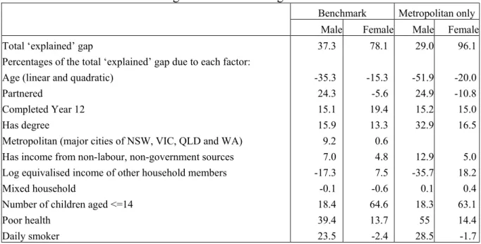
Table 6 reports the contribution of each factor in explaining the gap in labour market attachment between Indigenous and non-Indigenous Australians. The negative contribution of age in explaining the gap in labour market attachment between the two populations is due to the fact that Indigenous people are younger than non-Indigenous people and the fact that, on average, age has a negative effect on labour market attachment. A younger age structure is an advantage; all else equal, if Indigenous people had the same mean age as non-Indigenous people, their labour market attachment would be lower and the gap between the two populations wider. In other words, in contrast with other gaps such as that in life expectancy, age-standardising of the Indigenous and non-Indigenous demographic profile will widen the gap in labour market attachment.
Table 6: Contribution of each factor in explaining the gap in labour market attachment between Indigenous and non-Indigenous Australians
Benchmark Metropolitan only
Male Female Male Female
Total ‘explained’ gap 37.3 78.1 29.0 96.1
Percentages of the total ‘explained’ gap due to each factor:
Age (linear and quadratic) -35.3 -15.3 -51.9 -20.0
Partnered 24.3 -5.6 24.9 -10.8
Completed Year 12 15.1 19.4 15.2 15.0
Has degree 15.9 13.3 32.9 16.5
Metropolitan (major cities of NSW, VIC, QLD and WA) 9.2 0.6
Has income from non-labour, non-government sources 7.0 4.8 12.9 5.0
Log equivalised income of other household members -17.3 7.5 -35.7 18.2
Mixed household -0.1 -0.6 0.1 0.4
Number of children aged <=14 18.4 64.6 18.3 63.1
Poor health 39.4 13.7 55 14.4
Daily smoker 23.5 -2.4 28.5 -1.7
Note: Entries are percentages of the total ‘explained’ gap that are due to each factor.
Over two thirds of the ‘explained’ gap in labour market attachment between Indigenous and non-Indigenous women can be attributed to the fact that Indigenous women have more dependent children.25 Likewise, having poor health contributes 14 percent in explaining why
25 Or strictly speaking, live in households with more dependent children, since the children observed to live in the household are not necessarily the woman’s own children. Almost identical decomposition results are obtained when the number of children enters in log form, which allows the effect of an additional child to become smaller when more children are already present. In this latter case, the total explained gap is slightly smaller at 71.4 percent, but the proportion explained by the number of children increases slightly to 65.5 percent. For men, these percentages decrease to 35.7 percent and 13.7 percent respectively.
Indigenous women participate less in the labour market than their non-Indigenous counterparts. Other positive contributing factors include Year 12 completion and tertiary qualifications. Health and education are also important in explaining the gap in labour market attachment among men. For men, differences in partnering status are also important in explaining the difference between the two groups. Similar decomposition results are obtained when the analysis is restricted to metropolitan areas (Table 6, last two columns). It appears that health and education explain more of the gap in metropolitan areas, especially for men. The detailed decomposition suggests that the gap in outcome could be narrowed by closing the gaps in characteristics with positive contributions while widening the gaps in characteristics with negative contributions. Some changes that may be conducive to higher labour market attachment among Indigenous people are, for example, raising education levels, as well as reducing the incidence of poor health and family size (or alternatively, in the latter case, increasing support to care for children).
Some effects that the control variables in our models have on the outcome of interest are likely to reflect an association rather than direct causation. For example, partnership is associated with high labour market attachment among men, but it could be due to the unobserved characteristics that are associated with partnered men rather than the partnering status per se. Thus, increasing labour market attachment among Indigenous men could not simply be achieved by inducing them into a relationship.
7. Conclusions
This paper has used a novel approach of combining two separate data sets in a comparison between Indigenous and non-Indigenous Australians to increase the information available for both groups. The paper has analysed data from the 2008 NATSISS and HILDA (wave 8) surveys to examine the factors that affect the labour force status of Indigenous and non-Indigenous Australians in non-remote areas, and to decompose the gap in labour market attachment between the two populations into an explained (due to observed characteristics) and an unexplained component. Following a recently developed detailed decomposition approach (Powers, Yoshioka and Yun, 2011), we attribute the explained gap to differences in specific characteristics. Although the decomposition methodology is a descriptive approach and cannot determine causal relationships, insights into the factors that are associated with labour market attachment and that contribute to the gap between Indigenous and non-Indigenous Australians will be helpful in designing policies to "close the gap".
Significant factors that shape labour force status in both populations include age, education, health, smoking and number of children in the household. However, the size of the effects varies across genders and the two populations. The effects of the education variables are weaker for non-Indigenous people than for Indigenous people, whereas number of children in the household and poor health show stronger effects for non-Indigenous Australians.
Compared with previous studies, such as for example Hunter (2004), Daly (1993) and Miller (1989) who could explain one fifth to at most one third of the gap in employment, our study is able to explain more than half of the gap in employment between Indigenous and non-Indigenous men, and almost 80 percent of the gap between non-Indigenous and non-non-Indigenous women. This is due to the larger number of variables which are available from NATSISS and HILDA surveys compared to what is available in the Census (which was used in earlier studies).
The models based on the more detailed labour market attachment variable (distinguishing between not in the labour force, unemployment, part-time employment and full-time employment) explain at least two thirds of the gap in labour market attachment between Indigenous and non-Indigenous women. That is, even in this model with a more complex dependent variable to explain, a large part of the gap can be attributed to differences in the observed characteristics between the two populations. For men, the models only account for between 36 and 47 percent of the gap. This could be because other factors influence men’s labour market attachment than women’s and these factors may be absent from our models. In addition, the returns to characteristics between the two populations may be more different for men than for women, causing these to make up a larger proportion of the gap.
At least some of the remaining gap in labour market attachment of men is due to characteristics that are observed in the NATSISS data but not in the HILDA data, and therefore cannot be included in the analysis that attributes the gap in attachment to a range of observed factors. For example, the omission of arrest data is likely to be important in explaining some of the residual employment gap, given that Indigenous people are 11.5 times more likely to have been arrested than other Australians (Hunter and Daly, 2012). Given that Indigenous males are around three times more likely to have been arrested than Indigenous females, the effect of arrest is likely to be disproportionately affecting the male decompositions (Borland and Hunter, 2000).