Response Times Seen as Decompression Times in Boolean Concept Use
Jo¨el Bradmetz
University of Reims
Fabien Mathy
∗ Rutgers UniversityThis paper reports a study of a multi-agent model of working memory (WM) in the context of Boolean concept learning. The model aims to assess the compressibility of information processed in WM. Concept complexity is described as a function of communication resources required in WM (i.e., the number of units and the structure of the communication between units that one must hold in one’s mind to learn a target concept). This model has been success-fully applied in measuring learning times for three-dimensional concepts (Mathy & Bradmetz, 2004). In this study, learning time was found to be a function of compression time. To assess the effect of decompression time, this paper presents an extended intra-conceptual study of response times for two- and three-dimensional concepts. Response times are measured while using a previously learned concept. The model explains why the time required to compress a sample of examples into a rule is directly linked to the time to decompress this rule when categorizing examples. Three experiments were conducted with 65, 49, and 84 undergraduate students who were given Boolean concept learning tasks in two and three dimensions (also called rule-based classification tasks). The results corroborate the metric of decompression given by the multi-agent model, especially when the model is parameterized following static serial processing of information.
Mathy and Bradmetz (1999) (see also Mathy, 2002) con-ceived a multi-agent model of Boolean concept complexity and learnability accounting for both logical and psychologi-cal aspects of the problem (the complete set of Boolean con-cepts in two and three dimensions is shown in Figure 1). From a logical point of view, concepts are seen as the maximal compression of disjunctive normal forms. From a psychological viewpoint, conceptual activities are mod-eled through the specificity of working memory processing. Feldman (2000, 2003a) presents a very similar model also based on the study of the maximal compression of disjunctive forms. Mathy and Bradmetz (2004) compared Feldman’s model with a set of multi-agent models parameterized either in random, parallel, or serial mode. They showed that the
This research was supported in parts by two postdoctoral re-search grants from the Fulbright Program for Exchange Schol-ars and the Fyssen Foundation to Fabien Mathy. We thank the students of Rutgers University and those of Universit´e de Reims Champagne-Ardenne who kindly volunteered to participate in this study.
∗Correspondence concerning this article should be addressed to
Fabien Mathy, Center For Cognitive Science (RuCCS). Rutgers, The State University of New Jersey. Psychology Building Addition, Busch Campus. 152 Frelinghuysen road. Piscataway, NJ 08854, USA, or by e-mail at [email protected].
serial multi-agent model better predicted learning times for three-dimensional concepts.
The present article aims to reinforce the plausibility of the serial multi-agent model and to deepen the analysis of con-ceptual complexity by measuring the time needed to recog-nize each example of a given concept. Our hypothesis is that the time required to compress a sample of examples into a rule (i.e., the time to learn a rule) is directly linked to the time required to decompress this rule when categorizing exam-ples. Hence, this article switches from inter-conceptual com-parisons to intra-conceptual ones. Indeed, not only does the multi-agent model predict an ordering of conceptual com-plexity but also an ordering of example comcom-plexity for a given concept. To the best of our knowledge, this work has never been conducted on Boolean concepts. Before present-ing the multi-agent model, we define what is meant by com-pression and decomcom-pression and we also define their link to rule creation and rule use. We will also introduce a terminol-ogy that better describes the characteristics of the serial and parallel multi-agent models by calling them respectively the static serial model and the dynamic serial model. The differ-ence between the models is simple: The static serial model uses a fixed ordering of variables in the decision rule for a given concept, whereas in the dynamic model1the ordering 1There is an analogy with variable-typing in computer science.
Static-typed variables are defined at compile-time and remain
is flexible from one example to another. This leads to distinct measures of decompression time under the rules specified by the two models.
Rules, Algorithms and Compression
When categorizing stimuli, a weaker level of performance may be associated with a procedure equivalent to learning stimuli and their category by rote. For instance, in order to know if a number is even, one could divide this number by two, look at the remainder, and then note if the remainder is equal to zero. There is, however, a way of avoiding this kind of procedure which imposes a new calculation for each number: it is easier to tell if a number is even by considering only the last digit. This rule is “if the last digit is 0, 2, 4, 6, 8, then the number is even”. Such a rule is a compressed cal-culation in that it is a simplification that does not lead to any loss of information. Rule creation is the motor of conceptual progress in a lot of domains2. The opposite of describing a
sample of data by extension is for instance the genetic code or a set of axioms (e.g., geometry is based on the four Eu-clidian axioms, plus the optional fifth dealing with parallels). A second kind of compression derives from the fact that stimuli are not treated alike by a rule. Each stimulus may require a particular number of steps to be processed. This is very intuitive: to checkmate with a queen against the king is easier than with a knight and a bishop; using the Erathostene’s sieve method, it is easier to see that 1951 is a prime number than to see that 2209 is not because one has to reach 44 to know that 1951 is prime rather than 47 to know that 2209 is not; it is easier to recognize a gazelle in a herd of zebras than in a herd of antelopes, and so forth. This article will deal with this latter kind of compression. We will show that the time required to recognize a stimulus depends on the number of steps that have to be followed when using a given rule.
The following points describe the general problem that we will investigate:
1. Each rule is seen as an algorithm (a function), that may produce different output values depending on the given in-put values. (If the rule is “red=positive example” and if a red square is given in input, the rule will produce the output “positive example”)
2. Following the terms of the Port Royal logicians, each rule is taken to be a compressed definition of a concept. In this way, a rule (intension) is more compressed than the list of examples of a given concept (extension). (The rule “red = positive example” is more compressed than saying that “red square=positive example, red circle=
positive example, red diamond=positive example, etc.”) 3. Each rule may be more or less compressed, given that optimizations can be found to shorten the length of a rule. This paper assumes that all rules are compressed to the max-imum for the learning system considered.
4. Given a rule, some inputs require fewer steps to pro-duce an output. For instance, the rule “(red=positive) OR
(big blue diamonds=positive)” would take less time to in-dicate that a big red square is positive (there is one piece
of information to check) than to indicate that a big blue di-amond is positive (there are three pieces of information to check).
5. Given that a rule is a compressed number of operations that produces an output, the time to produce an output is a decompression time.
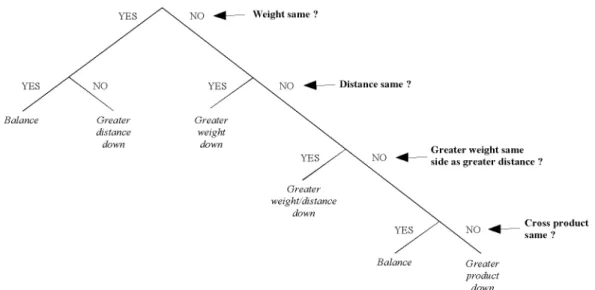
Let’s take a simple example requiring us to think about multiple dimensions: the balance scale problem (Inhelder & Piaget, 1955). Children are shown a balance scale, with spaced pegs along each side. A number of weights can be placed on the pegs. The correct solution to this problem is found by calculating the torque force on each side (i.e weight ×distance). Siegler (1981) identified several rules that chil-dren can possibly use to solve this problem. The most ad-vanced rule (that few adolescents use) is based on the torque on each side. This rule can be set as shown in Figure 2. Some paths in the decision tree are shorter than others: for exam-ple, if weights are equal and distances are equal as well, these two tests are sufficient to conclude that there is a balance. But then, there can be worse conditions in which the correct answer requires four tests (where all answers are “no”). This simple example shows that given a rule, the number of steps to get a correct response can vary and depends on the input values. Considering stimuli as input and the rule as an algo-rithm, the time the algorithm takes to run can be measured by a response time. Consequently, for a given algorithm, re-sponse times may depend on the number of conditions tested before getting an output.
Let’s take an example of this key idea applied to concept learning: Imagine that a white square, a white circle, and a black square are three positive examples of a concept, and that a black circle is a negative example. The minimal cor-responding disjunctive normal form (white∨square) is mod-eled in the majority of decision-rule models by the following rule: “if white then positive, if square then positive”. Only the static serial model that we will develop later leads to the different rule (if white then positive, if black then [if square then positive]) or equivalently (if square then positive, if circle then [if white then positive]). We see that two de-cisions are sometimes necessary in the two previous rules, which is not the case in the first one. The static serial model is not immediately intuitive and produces less compressed decision rules, but proves very economical when computing the biggest decision trees, due to the strict ordering of vari-ables it imposes.
changed throughout program execution, whereas dynamic variables are defined at run-time.
2Before Descartes, there was a procedure for each equation,
de-pending on the terms to the right and the left of the equals symbol. Descartes came up with a considerably more economical system of calculations by putting the terms on the left and a zero on the right. This discovery brought him up against the reticence of people to ac-cept that “something” could be equal to “nothing”. Here we see that all scientific revolutions take time. It took a couple of decades for Kepler to admit that planetary orbits were not circular, even though elliptical orbits actually simplified the calculus.
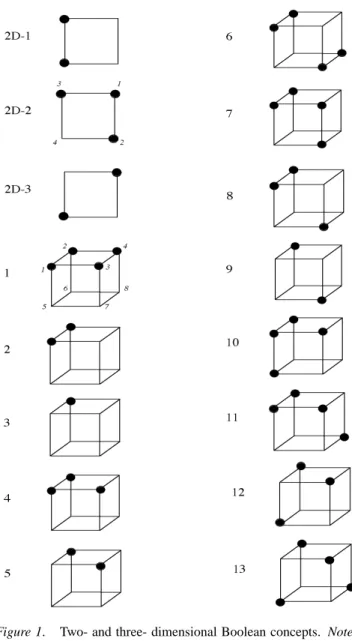
Figure 1. Two- and three- dimensional Boolean concepts. Note. positive examples are indicated by black circles; negative examples are empty vertices.
Compressibility and Complexity
The time to run an algorithm can be seen as a decompres-sion time. Let’s see how the notion of compresdecompres-sion can be inserted into a general theory called algorithmic complexity. Imagine N people represented in a diagram simply as dots and each two-way communication link as a line connecting two dots. The resulting diagram could be specified by the complexity of a pattern of connection. Everyone will agree that a pattern with a lot of connections is complex, but also that having all dots connected is just as simple as having no dots connected (Gell-Mann, 1994). This reasoning suggests that at least one way of defining the complexity of a sys-tem is to make use of the length of its description, since the phrase “all dots connected” is of about the same length as “no dots connected”. Computer scientists (e.g., Chaitin, 1974,
1987, 1990; Delahaye, 1993, 1994) consider a particular ob-ject described by a string of symbols and ask what programs will cause the computer to print out that string and then stop computing. The first and still classic measure of complexity that was introduced by Kolmogorov is roughly the shortest computer program capable of generating a given string (Kol-mogorov, 1965). The length of the shortest program is the algorithmic complexity of the string or “Kolmogorov com-plexity”. It corresponds to the difficulty of compression of a representation. Some strings of a given length are incom-pressible. In other words, the length of the shortest program that will produce one of these strings is one that says PRINT followed by the string itself. Such a string has a maximum Kolmogorov complexity in relation to its length, given that there is no algorithm that will simplify its description. It is called a random string precisely because it contains no regu-larity that enables it to be compressed.
Kolmogorov complexity is a measure of randomness, but randomness is not what is usually meant by complexity. In fact, it is just the nonrandom aspects of an object that con-tributes to its effective complexity (e.g., its structure), which can be characterized as the description of the regularities of that object. Bennett complexity shadows this type of com-plexity linked to the fact that an object can be highly struc-tured, but still difficult to compute. The inadequacy of Kol-mogorov complexity is striking when considering that the complexity of a string can be very high in view of the compu-tation it needs even if the program is very short. For instance, the string of the first hundred million digits ofπhas a small Kolmogorov complexity, but the time needed for the program to produce the digits is high. A fractal can also be represented by a short algorithm, but it takes a long time to compute. This complexity is linked to the difficulty of computation: the complexity is low since the algorithm has few computa-tions to do. This computational content is called organized complexity, logical depth or Bennett complexity (Bennett, 1986). Bennett complexity can be summed up by the time taken to decompress an object described by a minimal algo-rithm. In physics, the question of existence of regularities in the world reduces to knowing if the world is algorithmically compressible (Davies, 1989; Wolfram, 2002). It is hence reasonable to ask wether our mental model of the world is itself an algorithmic compression. Taking into account that a rule is an algorithm, Kolmogorov and Bennett complexity are two complementary ways of understanding the complexity of objects to be learned by using rules. That much of induction processing concerns compression is a “unifying principle” across many areas of cognitive science (Chater & Vit´anyi, 2003) and is very useful in many applications (Li & Vit´anyi, 1997). We will see that the length of a rule compressing the structure of a concept and its decompression time are esti-mates of the Kolmogorov and the Bennett complexity of this concept.
Concept Learning
This research focuses on the ability to successfully dis-cover and use arbitrary classification rules, also called
con-cept learning tasks (Bourne, 1970; Bruner, Goodnow, & Austin, 1956; Levine, 1966; Shepard, Hovland, & Jenkins, 1961). In concept learning, learners are shown a sequence of multidimensional stimuli and formulate a hypothesis con-cerning the instances which do or do not belong to a cat-egory, until they inductively reach the target concept. The three basic types of classification rules in two dimensions are presented in Figure 1, as well as the thirteen in three dimen-sions. Each vertex may represent the combination of Boolean input variables leading to compound stimuli wherein shape, color and size are amalgamated. For instance, four figures would be generated from two binary dimensions each hav-ing two values. The value of the two category responses are represented in Figure 1 by black circles (positive examples) and vertices without black circles (negative examples). A concept is thus thought of as the set of all instances that pos-itively exemplify a classification rule.
A learning system may compress the information held by different conceptual structures into simple rules, depending on the sum of the regularities present in those structures. We develop here several multi-agent models deriving from deci-sion tree processing to show how humans compress concepts using simple rules but why they do not compress them using the simplest rules. We will see that this fact is closely linked to the computation demanded when inducing concepts3.
Multi-agent Models of Concept Learning
In studying structural biases in concept learning, one in-vestigates the system of relations in the concept to be learned and asks how the organization of relations might affect learn-ing processes. The concept of structure is not easy to grasp: the perception of structure is a quite different matter from the perception of shapes or other physical stimuli (Lockhead & Pomerantz, 1991). A structured system can be defined as one that contains redundancy. To assess whether a learn-ing system might compress the information held by concep-tual structures, Feldman (2000) proposed a metric based on logical incompressibility, i.e. by defining a maximally com-pressed disjunctive normal formula for each concept. He showed that conceptual difficulty reflects intrinsic logical complexity on a wide range of concepts (up to four dimen-sions). Using a model inaugurated by Mathy and Bradmetz (1999), Mathy and Bradmetz (2004) have evaluated Feld-man’s model with respect to a series of multi-agent mod-els developed to be analogous to the functioning of work-ing memory. The inherent advantage of multi-agent models is that they allow one to address the issue of the nature of information processing (static serial, dynamic serial, or ran-dom) to compute logical formulas. They showed that the different models offer several ways of compressing a given sample space using a logical formula. The results also indi-cated that the dynamic serial model leading to the most com-pressed formulas does not give the best fit with the experi-mental data. Conversely, the results confirmed that the static serial model, which imposes a fixed information-processing order, is the best model to fit the data, even if it does not lead to the maximal compression of information compared to
the dynamic serial model. The aim of this paper is to verify this result in a completely different context of measurement, moving from inter-conceptual measures of learning times to intra-conceptual measures of response times.
Let’s sum up the writing of communicational protocols in the multi-agent model of working memory proposed by Mathy and Bradmetz4. The main idea that underpins the
model is that agents enable common knowledge to be elabo-rated from distributed knowledge. As in classical distributed systems in which processing is split up, each agent can be seen as a working memory unit that merely receives infor-mation from a given dimension and that is blind to others. However, common knowledge made up of several pieces of information is usually necessary to solve problems. Hence, agents have to communicate as the need arises to coordinate information and progressively adapt a minimal communica-tion structure to the problem5. The communication demand can hence be a measure of information complexity held by a concept (see Hromkoviˇc, 1997, for a development of com-municational complexity).
3In artificial intelligence, a theoretical analysis of inductive
rea-soning has been introduced by Gold (1967). Gold developed the notion of convergence (identification in the limit) by understanding that the most accurate hypotheses are reached faster when begin-ning to test the smallest ones (see also Osherson, Stob & Weinstein, 1986, for a development of Gold theories). This principle, which consists of choosing the simplest rules is known as Occam’s ra-zor: it guarantees both fast learning and accurate generalizations (see a study of simplicity principle in unsupervised categorization in Pothos & Chater, 2002; a study of learning based on the prin-ciple of minimum description length (MDL) in Fass & Feldman, 2002; Feldman, 2003b for a short introduction to simplicity prin-ciples in concept learning and Feldman, 2004, for a study of the statistical distribution of simplicity). Lately, computational learn-ing theories have achieved success with the probably approximately correct (PAC) learning theory of Valiant (1984) (Anthony & Biggs, 1992; Hanson, Drastal & Rivest, 1994; Hanson, Petsche, Kearns & Rivest; Kearns & Vazirani, 1994). This approach gives a formal background (integrating statistical concepts, Vapnik-Chernovenkis dimensions, etc.) to a lot of theories from neural networks to in-ductive logic programming (De Raedt, 1997). A second approach, which we will follow in this paper, aims to develop symbolic learn-ing algorithms based on decision trees, and is very well suited to the non-fuzzy Boolean concepts studied here (Quinlan, 1986; see Mitchell, 1997, for a general presentation or Shavlik & Dietterich, 1990, for readings in machine learning).
4We will not present the method for obtaining communication
protocols, as it is already explained in Mathy and Bradmetz (2004). The method is based on computing the information gain for each piece of information given by agents until there is no more uncer-tainty about the class. The knowledge of an agent is computed by the conditional entropy quantifying the remaining uncertainty about the class once its knowledge is made public.
5This progressive adaptation recalls “in the spirit” the procedure
of identification in the limit, Gold, 1967, the algorithm cascade cor-relation for neural networks, Fahlman & Lebiere, 1990, the RULEX model that begins with the simplest rules and adds exception if nec-essary, Nosofsky, Palmeri & McKinley, 1994, and the SUSTAIN model of category learning in which clusters are recruited progres-sively, Love, Medin & Gureckis, 2004).
Figure 2. Siegler’s (1981) flow chart that describes the most advanced rule based on the torque force on each side of a balance.
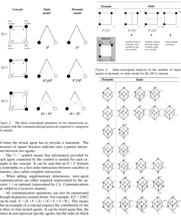
For example, let’s consider the two-dimensional Boolean world based on two shapes and two colors. Following the conceptual structures in Figure 3, it is assumed that the two stimuli on the left are blue, the two on the right are red, the two top ones are triangles, and the two bottom ones are cir-cles. The concept 2D-1 is modeled by a unary communi-cation protocol X4, because, only one agent (here the shape agent) is required to sort the stimuli according to their shape. Both dynamic and static models lead to the same formula. The decision tree associated with the formula means that, if the stimulus is a triangle, X will follow the left branch and conclude that the stimulus is a triangle (because the leaf is marked with a positive symbol); in the case where the stim-ulus is a square, X will follow the right branch and conclude that the stimulus is a negative example of the concept (the leaf is a negative example). Because X is required four times (for a single presentation of the training sample), the expo-nent is equal to four. Note that here we only present the for-mula once it has been discovered by the multi-agent model, avoiding all the discovery processes.
Let’s explain concept 2D-2 now labeled X4[Y]2 for the static serial model: the embedded communications neces-sary for this concept lead to a partial interaction between two agents. The first possibility is that the color agent speaks first. For the two red stimuli, the color agent (X ) will be sufficient to conclude that the stimuli are positive examples by following the left branch. In contrast, when speaking first for the blue ones, the color agent leaves one bit of informa-tion. The second speaker Y (the shape agent) will complete the task in following the left dotted line when the stimulus is triangle and the right one if it is a square. (The same com-munication protocol and the same decision tree holds if the shape agent speaks first). Given that the second speaker is required only twice, we can set the exponent to 2. The ...[...] binary operator indicates that Y is not required all the time: the interaction between X and Y is partial. The formula for the dynamic serial model is more compressed X4[Y]1: The
advantage of the dynamic serial model is that agents are not constrained by a fixed order of communication. The root rep-resents the choice to be made by the first speaking agent X , no matter who he is. For that reason, both the color and the shape agents can replace X . The color agent is sufficient to categorize the red stimuli as positive example and the shape agent is also sufficient to categorize the triangle stimuli as positive examples (one of the two agents is randomly cho-sen for the red square). In contrast, the red circle stimulus requires two agents to be sorted because an interpretation of silence is not allowed in this model (either the color agent gives its piece of information followed by the shape agent, or the shape agent gives its piece of information followed by the color agent). The best way to structurally represent dynamic serial formulas is to see them as decision trees in which the same path could be followed by several agents. X4[Y]1 therefore means that an agent X is required for all stimuli, but also that an optional agent is needed to classify one of the stimuli. The 2D-3 concept could be modeled by a X4[Y]4formula, but in view of the fact that two agents are required for all stimuli, a new binary operator representing a complete interaction gives the following formula X4∧Y4or simply(X∧Y)4. The same principles lead to the formulas in three dimensions. All formulas are given in Table 1.
Several key assumptions are made to describe formulas associated with each concept:
- Formulas represent the minimal inter-agent communica-tion protocols.
- Embedded communications are reduced to a communi-cation between a first speaker, a second speaker and so forth Each letter X , Y (and so on) stands respectively for the first and the second speaker (and so on). The number of letters (i.e. the number of agents) directly represents the number of units in working memory that are required in concept learn-ing.
- The square brackets indicate that the speaker is optional and the exponent linked to the bracket indicates the number
Figure 3. The three conceptual structures in two dimensions as-sociated with the communicational protocols required to categorize all stimuli.
of times the nested agent has to provide a statement. The presence of square brackets indicates also a partial interac-tion between two agents.
- The “∧” symbol means that information provided by each agent connected by the symbol is needed for each ex-ample in the concept. It can be said that an X∧Y formula is isomorphic to a first order interaction between variables in statistics, also called complete interaction.
- When adding supplementary dimensions, inter-agent communications are either required (represented by the op-erator∧) or optional (represented by [ ]). Communications are added in a recursive manner.
- All communication operations can also be enumerated through disjunctive normal forms. For example, X[Y∧Z[W]]
can be read: X∨(X∧Y∧Z)∨(X∧Y∧Z∧W). This means that an example of a concept requires the contribution of one or three or four nested agents. It can be noted again that, the letters do not represent specific agents, but the order in which information is given.
Figure 4 and Figure 5 indicate the number of required agents for each concept, when the dynamic and the static models lead to different patterns. As regards the fact that dimensions are chosen randomly, we assume that one can compute a mean number of required agents to classify a
stim-Figure 4. Intra-conceptual analysis of the number of required agents in dynamic or static mode for the 2D-2 concept.
Figure 5. Intra-conceptual analysis of the number of required agents in dynamic or static mode for concepts 2, 3, 4, 5, 8, 11, and 12. Orders 1, 2, and 3 of the static model are shown from left to right. When six orders were possible, they have been averaged by pairs to produce a maximum of three orders.
Table 1
Dynamic and static communication protocols associated with two- and three- dimensional concepts.
Concept Dynamic Static
2D-1 X4 X4 2D-2 X4[Y]1 X4[Y]2 2D-3 X4∧Y4 X4∧Y4 1 X8 X8 2 X8[Y]2 X8[Y]4 3 X8[Y[Z]1]1 X8[Y[Z]2]4 4 X8[Y[Z]1/3]4 X8[Y[Z]2]4 5 X8[Y[Z]2]4 X8[Y∧Z]4 6 X8∧Y8 X8∧Y8 7 X8∧Y8 X8∧Y8[Z]4 8 X8∧Y8[Z]1 X8∧Y8[Z]2 9 X8∧Y8[Z]2 X8∧Y8[Z]4 10 X8∧Y8[Z]2 X8∧Y8[Z]4 11 X8∧Y8[Z]2 X8∧Y8[Z]4 12 X8∧Y8[Z]4 X8∧Y8[Z]6 13 X8∧Y8∧Z8 X8∧Y8∧Z8 Sum= 201.3 224
Note. Bold lines indicate that the dynamic serial model and the
static serial model lead to different theoretical patterns of mean response times. The patterns of intra-conceptual response times are not automatically distinguishable when formulae are different.
ulus. In Figure 4 for example, assuming that we run the multi-agent model several times, 50 % of the time two agents will be necessary to classify the stimulus 2 if the color agent speaks first whereas one agent will be sufficient if the shape agent speaks first, leading to a mean number of agents of 1.5. The same rule has been applied to all concepts in three dimensions in Figure 5. Dotted lines indicate the separation made when the first agent gives its piece of information. We make the assumption that the number of pieces of informa-tion for each stimulus indicated in Figures 5 can easily be recovered from the analysis of response times once a concept is learned.
The first experiment was conducted to measure response times of each instance of the previously learned 2D-2 con-cept and compare them to intra-concon-ceptual patterns of the theoretical number of agents in the static and the dynamic model. The second experiment aimed to measure response times of 3D concepts (2, 3, 4, 5, 8, 11, 12) which also lead to different intra-conceptual patterns of the number of agents in the static and the dynamic models. The third experiment was designed to contrast the static serial model (which turns out to be the more accurate in the first two experiments) with an exemplar model. The relation between these models is peculiar for concept number 10: For instance, the mean theo-retical response times produced by both models are perfectly correlated for this concept. Only an analysis of subject pat-terns of response times is able to discriminate the models. In these three experiments, response times were measured while subjects were using a previously-learned concept.
EXPERIMENT 1:
Two-dimensional Concept
Application
Mathy and Bradmetz (2004) did not make the distinction between learning stimuli and categorizing them after the con-cept is learned. The present experiment was thereby de-signed to address the question of intra-conceptual response times in a previously learned concept. The objective here was to show that stimuli require different response times to be categorized, because the number of pieces of information to be given for each stimulus can be different according to the multi-agent model. The second goal was to determine which multi-agent model (dynamic versus static) is best able to de-scribe the pattern of response time per stimulus. We chose to begin with the 2D-2 concept which led to different theo-retical patterns of numbers of agents in the static and the dy-namic models. It is important to understand that the number of pieces of information required to identify each instance of a concept in the multi-agent models is assumed to be defined once the communication protocol is established (i.e. once the concept is learned). Accordingly, the responses times were measured after a given criterion had been met which guar-antees that the target concept had been learned and could be applied without error.
Method
Participants
This experiment included 65 students. All participants were high school students or university undergraduates who participated voluntarily.
Stimuli
It is worth mentioning that a correct embodiment of physi-cal dimensions is quite important in testing the cumulative ef-fect of several dimensions in working memory. In this study, input variables were compound stimuli wherein shape, color, size and a frame were amalgamated. In 2D (see stimuli in Figure 6), figures varied along two binary dimensions each having two values, leading to a sample of four figures (e.g., a red square, a blue square, a red circle and a blue circle). The colors and shapes of the different concepts were randomly chosen from a set of values (triangle, square, oval, blue, pink, red, green, circle frame, diamond frame).
Procedure
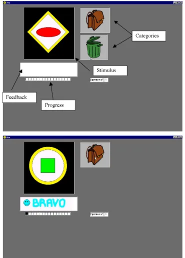
Tasks were computer-driven. On the day of the exper-iment, participants looked at tutorials on a computer that taught them basic computer skills, how to sort stimuli in the two locations (either a school bag or a trash can) and how to succeed with a classification (fill up all the progress bar). The stimuli were then presented in a window on the left of the school bag and the trash can (see Figure 6). When participants chose to classify a stimulus by clicking on the school bag (or the trash can), the picture of the trash can (or the school bag) disappeared to facilitate the association of
stimuli to their respective category. Feedback was provided at the bottom of the screen, indicating if the response was right or wrong and adding a picture of a smiling or an an-gry man. Each correct response scored them one point on a progress bar. A point was represented by an empty box that was filled in when they gave a correct response. The number of points in the progress bar dedicated to learning was equal to twice the length of the training sample, that is 2×2N(N =
number of dimensions). Once the concept had been learned, response times were measured on a further 2×2N points.
Consequently, subjects had to correctly categorize stimuli on four consecutive blocks of 2N stimuli. For example,
partic-ipants learning a 2D concept had to fill up a progress bar of 16 points, without even knowing that reaching 8 correct responses was the learning criterion and that response times were measured during the 8 next correct responses.
Each response had to be given in less than 8 seconds, oth-erwise the participants would lose 3 points on the progress bar. When they gave a wrong response, the participant would lose all points scored. Finally, they were rewarded with a digital image (animals, fractals etc.) when they succeeded. In Experiment 1, the stimuli varied along 2 binary-valued di-mensions (see the four stimuli in Figure 6). In each block of 2N stimuli, each stimulus appeared once in a random order, and the first stimulus of each block was different from the last of the previous block. An assignment of physical dimensions was randomized for each concept and each subject. In Exper-iment 1, all subjects were invited to learn the 2D-2 concept after a short warm-up trial.
Results
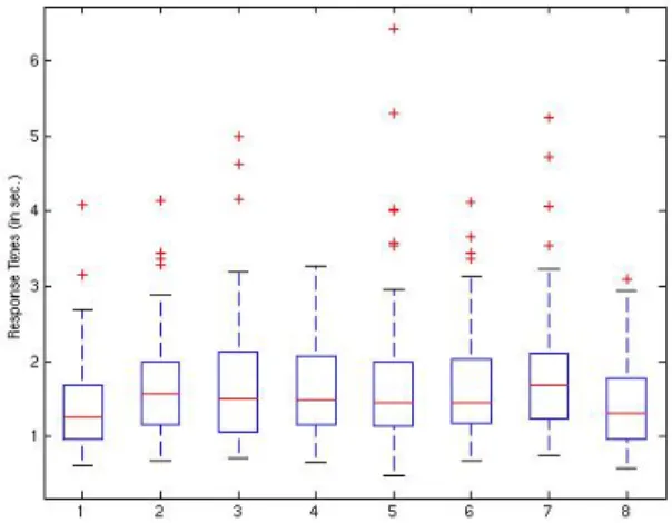
With respect to the analysis of dispersion of response times, there was a great deal of variability in the data (see Boxplots in Figure 7). Positively skewed patterns came from a few extreme scores corresponding to subjects who took more time to respond. Consequently, we indicate in Ta-ble 2 median response times and base-e logarithms of re-sponse times to avoid the effect of these extreme scores on mean response times. Median response times or base-e loga-rithms of response times show a very good fit with the num-ber of agents per stimulus6 predicted by the static model.
That is, the response times have higher medians for stimuli that require more pieces of information. The within-subjects analysis of variance applied on base-e logarithm response times proves that stimuli are not categorized at the same rate (F(3,192) =5.16; p=.002).
The results, shown in Table 3, indicate that the static model shows a better fit with the median times. To test the agreement of data with the dynamic or static models, we computed correlations between the mean response times per subject and the number of agents per stimulus for each pat-tern of the static and the dynamic models. Then, we searched which mode (dynamic vs. static) was the closest to the sub-ject patterns (a pattern for a given subsub-ject is the set of em-pirical response times for a given concept). Note that in the static mode, there are two theoretical patterns corresponding to the two manners of ordering the variables in the 2D-2
con-Figure 6. Screen shot of windows in Experiments 1, 2, and 3.
cept (as shown in Fig. 4). Then we counted the number of times the static model turned out to be superior to the dy-namic serial model. The results are shown in Table 3. For the 2D-2 concept, the results go against the dynamic serial model: on 50 (order 1: 30; order 2: 20) occasions out of 65 the response times are closer to the static serial model
(χ2(1) =18.8; p< .001). Thus, the static model proved to
be significantly superior to the dynamic one, with a greater correlation between the number of required agents per stim-ulus and the response times. This points out the merits of modeling information processing in working memory using distributed models that process information in a fixed order.
Discussion
It is assumed that the processing of dimensions by work-ing memory units directly corresponds to the work of simple agents that use minimal inter-agent communications to iden-tify and classify each example of target concepts. The multi-agent model takes into account the number of units required 6The numbering of stimuli used in Table 2 (Ex1, Ex2, Ex3 and
Table 3
Number of patterns by subject that fit either the static model or the dynamic one.
D Concept nDyn. nStat. Order1 Order2 Order3 χ2(1) rMed.SM rMed.DM
2D 2D-2 15 50 30 20 - 18.8∗∗∗ .985∗ .706 3D 2 13 36 15 21 - 10.8∗∗∗ .744∗ .732∗ 3D 3 12 37 16 12 9 12.8∗∗∗ .980∗∗ .869∗∗ 3D 4 10 39 39 - - 17.2∗∗∗ .943∗∗ .920∗∗ 3D 5 15 34 34 - - 07.4∗∗∗ .929∗∗ .730∗ 3D 8 4 45 23 22 - 34.3∗∗∗ .106 .083 3D 11 10 39 27 12 - 17.2∗∗∗ .783∗ .538 3D 12 6 43 16 11 16 27.9∗∗∗ .552 .393
Note. D, number of dimensions; nDyn., number of patterns by subject that fit the dynamic model; nStat., number of patterns by subject that
fit the static model; rMed.DM, correlation between the median response times given in Table 4 and the number of agents per example in the
dynamic model; rMed.SM, correlation between the median response times given in Table 4 and the mean number of agents per example in the
static model;∗∗∗significant at the 0.001 level;∗∗significant at the 0.01 level;∗significant at the 0.05 level; Order1, Order2, and Order3 are represented in Figure 5 and Figure 10.
Figure 7. Boxplots of response times for both positive and nega-tive examples of the 2D-2 concept. Note. The stimulus labels 1, 2, 3, and 4 are given in Figure 1.
Table 2
Response times for both positive and negative examples of the 2D-2 concept studied in Experiment 1.
1∗ 2 3 4 Mean RT 1.22 1.41 1.45 1.58 SD (RT) .64 1.57 .69 .69 Mean LN(RT) .11 27 .27 .38 Median RT 1.04 1.29 1.30 1.45 Static 1 1.5 1.5 2 Dynamic 1 1 1 2
Note. RT, Response times; SD, Standard deviation of mean time;
Static, mean number of agents per example required by the static model; Dynamic, number of agents per example required by the dynamic model; *, examples 1, 2, 3, and 4 in the 2D-2 concept are indicated in Figure 4. Bold lines indicate the closest patterns.
per example and the number of communications used to clas-sify each example. A distinction can be made according to whether communications are dynamic serial (when there is no order constraint between agents for the whole concept) or static serial (when a fixed ordering between agents is im-posed for the whole concept). When response times were measured after the concept was learned, the results showed that the static serial model yielded a valid measure of adult processing speed when categorizing stimuli. Indeed, the the-oretical computation of the number of pieces of information per example (when processing is static) seems to predict pat-terns of response times for the 2D-2 concept. When theo-retically comparing the number of agents required for each example of the 2D-2 concept, a clear outcome is that static serial processing of information leads to a less compressed communication protocol formula than the one given by a dy-namic serial model. This finding indicates that lower rule compressions may be privileged by human learners. This is certainly due to the reason invoked by Mathy and Brad-metz (2004): static serial processing in the multi-agent model leads to lower compressions of communication protocols but communication protocols are generated faster by the system. When learning concepts people would have a better perfor-mance at the end using the dynamic method, but the time required to learn the concept would be greater7.
In conclusion, the measure of response times (once the 2D-2 concept has been induced) sheds lights on a basic com-munication protocol between two memory units processing information in a static serial way. The time needed to cate-7Let’s make an analogy: when memorizing before dialing a
phone number, it takes less time to dial a number after its entire memorization (let’s imagine 6 seconds to memorize the entire num-ber plus 3 seconds to dial, for a total of 9 seconds), than to quickly look up and memorize the numbers and dial them group by group (e.g. 4 groups, and 3 sec. per group, for a total of 12 seconds). Nevertheless, a lot of people choose the second solution because starting to memorize an entire number takes more time (i.e., 6 sec-onds in our example) than directly memorizing the first group (i.e., 3 seconds) and then dialing it (of course, this analogy should be experimentally examined).
gorize each stimulus can be seen as a decompression time for this communication protocol. To classify the positive exam-ples, the corresponding decision rule of this static communi-cation protocol is “if x1then ex+, if x2then [if y1then ex+]”. This is not intuitive compared to the more compressed rule produced by the dynamic model (if x1then ex+, if y1 then ex+). The rule produced by the dynamic model is equiva-lent to the minimal disjunctive normal form (DNF). Conse-quently, this result casts doubt on models that use compres-sion of DNF as a metric of conceptual complexity (cf. Feld-man, 2000). This result also runs contrary to models based on neural networks: A simple perceptron would obviously set the weights on x1and y1to sufficient values to make the output fire for x1, y1, or both.
EXPERIMENT 2: Application of
Three-dimensional Concepts
Experiment 1 clearly indicated that adults learn two-dimensional concepts by following the static serial measure of intra-conceptual communication complexity given by the multi-agent model. Experiment 2 aimed to assess whether these same findings remain valid when the target concepts are based on three dimensions.
Method
Participants
This experiment included 49 students, different from those who took part in Experiment 1.
Procedure
Using the learning program described in Experiment 1, each participant was tested under 13 treatment conditions corresponding to the 13 concepts in 3 dimensions. Tasks were undertaken in 7 sessions, one session per day. The stimuli varied along 3 binary-valued dimensions, i.e. shape, color and frame (see stimuli in Figure 6). The assignment of physical dimensions was randomized for each concept and each subject. The presentation order of concepts was coun-terbalanced to reduce the risk of carry-over effects from one concept to the next. Following the criteria described in Ex-periment 1, participants had to fill up a progress bar of 32 points. The response times were measured for the last 16 correct responses. Finally, they were rewarded with a digi-tal image (animals, fracdigi-tals etc.) when they succeeded. Only then were they able to pause before learning another concept.
Results
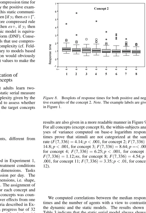
We have conducted an analysis of response times for the concepts listed in Figure 5 because they lead to different theoretical intra-conceptual patterns in the dynamic and the static model. Boxplots of Figure 8 show positively-skewed patterns of response times similar to those observed in Exper-iment 1, simply indicating that some subjects took more time to respond. Dispersion of response times is analogous for all other concepts. Descriptive statistics are given in Table 4 (the
Figure 8. Boxplots of response times for both positive and nega-tive examples of the concept 2. Note. The example labels are given in Figure 1.
results are also given in a more readable manner in Figure 9). For all concepts (except concept 8), the within-subjects anal-yses of variance computed on base-e logarithm response times prove that stimuli are not categorized at the same rate (F(7,336) =4.14; p< .001, for concept 2; F(7,336) =
14.8; p< .001, for concept 3; F(7,336) =8.64; p=< .001,
for concept 4; F(7,336) =6.25; p< .001, for concept 5; F(7,336) =1.12; ns, for concept 8; F(7,336) =4.54; p< .001, for concept 11; F(7,336) =3.35; p< .01, for concept 12).
We computed correlations between the median response times and the number of agents with a view to contrasting the dynamic and the static models. The results shown in Table 3 indicate that the static serial model always shows a better fit with the median response times with higher correla-tions. We also investigated which mode (dynamic vs. static) was the closest to the subject patterns. As far as the static serial model is concerned, there were several patterns corre-sponding to the several possible ways of ordering the vari-ables (between two and six orderings, averaged by pairs, as shown in Fig. 5). As in Experiment 1, we counted the num-ber of times the static serial model turned out to be superior to the dynamic serial model by computing the correlations between the mean response times per subject and the num-ber of theoretical agents per stimulus. The results given in Table 4 show a decided difference between the dynamic and the static models: For all concepts in 3D, the static serial model better suited the data.
Table 4
Means and median response times of both positive and negative examples of concepts 2, 3, 4, 5, 8,11,12 (in Exp. 2) and concept 10 (in Exp. 3) once they are learned.
Concept 2 Concept 3 Concept 4 Concept 5
M Me SM DM M Me SM DM M Me SM DM M Me SM DM Ex1 1.31 1.21 2 2 0.93 0.86 2 1 1.40 1.21 2 2 1.55 1.38 3 2 Ex2 1.26 1.09 2 2 1.13 1.08 3 3 1.51 1.32 2.5 2 1.49 1.27 3 3 Ex3 1.11 1.11 1.5 1 0.81 0.75 1.3 1 1.44 1.29 2.5 2 1.39 1.35 3 3 Ex4 1.16 1.02 1.5 1 0.86 0.82 2 1 1.58 1.37 3 2.3 1.59 1.53 3 2 Ex5 1.09 0.88 1.5 1 0.80 0.74 1.3 1 1.11 0.99 1 1 1.05 0.99 1 1 Ex6 1.09 0.90 1.5 1 0.91 0.84 2 1 1.23 1.15 1 1 1.19 1.09 1 1 Ex7 1.01 0.93 1 1 0.78 0.69 1 1 1.21 1.07 1 1 1.22 0.99 1 1 Ex8 0.95 0.88 1 1 0.76 0.71 1.3 1 1.16 1.01 1 1 1.25 0.99 1 1
Concept 8 Concept 11 Concept 12 Concept 10 (Exp, 3)
M Me SM DM M Me SM DM M Me SM DM M Me SM EM Ex1 1.60 1.40 2 2 1.52 1.28 2 2 2.00 1.90 3 3 1.26 1.38 2 1.22 Ex2 1.50 1.37 2 2 1.55 1.43 2.5 2 1.75 1.44 3 3 1.58 1.68 2.66 1.56 Ex3 1.54 1.50 2.5 2 1.78 1.64 2.5 2 1.69 1.49 3 3 1.51 1.74 2.66 1.56 Ex4 1.38 1.33 2 2 1.88 1.73 3 3 1.73 1.57 2.6 2 1.49 1.64 2.66 1.56 Ex5 1.63 1.63 2 2 1.45 1.26 2 2 1.80 1.60 3 3 1.46 1.74 2.66 1.56 Ex6 1.46 1.26 2 2 1.57 1.35 2.5 2 1.68 1.48 2.6 2 1.45 1.67 2.66 1.56 Ex7 1.53 1.43 3 3 1.78 1.66 2.5 2 1.77 1.56 2.6 2 1.68 1.76 2.66 1.56 Ex8 1.50 1.33 2.5 2 1.70 1.57 3 3 1.53 1.33 2 2 1.32 1.43 2.66 1.22
Note. EM, theoretical response times for the exemplar model; M, Mean response times; Me, Median response times; SM, mean number of
agents in the static model; DM, number of agents in the dynamic model. Bold columns indicate the closest patterns.
EXPERIMENT 3: Static Serial
Model versus Exemplar Models
Links to Prototype and Exemplar Models of
Cate-gorization
Exemplar models, as opposed to prototype models, are very well suited to nonlinearly separable concepts, like some of those in this study. These models are a generalization of the prototype models because they assume that the exemplar that has the highest probability to belong to a category is the prototype. However, it is difficult to understand the role of a prototype in that case because the prototype does not provide a good summary of the category members (Yamauchi, Love and Markman, 2002). In exemplar models, categorization is based on the computation of similarities within a set of ex-emplars stored by subjects (for a review, see Hahn & Chater, 1997). According to similarity-based approaches, the more similar an item is to what is known about a category, the more likely this item will be placed in this category. Exemplar models are also called context models because exemplars form a context for computing similarities between an item and each exemplar of a category (Estes, 1994; Kruschke, 1992; Medin & Schaffer, 1978; Nosofsky, 1986; Nosofsky, Gluck, Palmeri, McKinley, & Gauthier, 1994; Nosofsky, Kr-uschke & McKinley, 1992).
Following Nosofsky’s (1986) generalized context model of categorization(GCM), exemplars are represented in a psy-chological space. Distance between two stimuli i and j is given by the Minkowski metric
di j= [ n
∑
a=1
|xia−xja|r]1/r (1)
where r=1 when the distance is city-block, and where xiais the value of stimulus i along dimension a. Similarity
ηbetween two stimuli i and j is an exponentially decreasing function (called the exponential decay function) of psycho-logical distance
ηi j=exp−di j (2)
This decay function is better adapted to the city-block metric (Shepard, 1987). Given the total similarity of a stim-ulus s to all exemplars of categories X and Y , the probability of responding with category X is given by Luce’s choice rule:
P(X/s) = ∑x∈Xηsx
∑x∈Xηsx+∑y∈Yηsy
(3) In order to make a comparison with the static serial model, we computed the similarities among stimuli in all Boolean concepts studied in Experiments 1 and 2 using the three equa-tions above. We used a city-block metric (adequate for sepa-rable dimensions) in a traditional multi-dimensional scaling model (Minkowski Metric), and transforming similarities in probabilities by the Luce’s (1963) choice rule (cf. chapter 10 in Lamberts, 1997). We found that probabilities of classifi-cation of exemplars are inversely related to the mean num-ber of pieces of information for the static serial model. That is, the exemplar ex1 in Figure 4 has the highest probability of being classified as a positive example and is considered
Figure 9. Theoretical intra-conceptual analysis of the number of required agents in dynamic and static mode for the concepts 2D-2, 2, 3, 4, 5, 8, 11, 12 and empirical results given as median response times per example.
a prototype. Exemplars ex2 and ex3 are equally considered as having a medium probability of being positive examples and ex4 has the lowest probability of being classify as a neg-ative example. If we hypothesize as Nosofsky and Palmeri (1997) and Nosofsky and Alfonso-Reese (1999) successfuly did, that the response times depend on the similarity pattern of a stimulus to the exemplars from both categories, the pat-tern given by the exemplar model is very similar to the one given by the mean static serial model. Simply put, the in-verse probabilities given by the exemplar model can be seen as measures of response time and are correlated with the
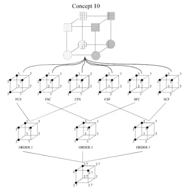
the-Figure 10. Modelisation of concept 10 by the static serial model.
Note. F, filling; C, color; S, Shape; FCS means that the order of decisions is filling, color, and shape.
oretical response times determined by the static model (cf. last column in Table 5).
Experiments 1 and 2 showed that the static serial model best fits the data of the present study. We will therefore con-sider only the static model as a comparison with the exemplar model. The major difference between the exemplar models and our static serial multi-agent model is that mean theoret-ical patterns of response times in the static serial model is a mixture of several static serial strategies that may be used by subjects, whereas the exemplar model computes just one pattern.
In this experiment, we compare the static serial model to GCM. Concept 10 serves as a basis for the comparison be-tween the two models, as the patterns of theoretical response times they produce are perfectly correlated for this concept. A second advantage of this concept is that the six possible orders of variables lead to the same equivalent decision trees. These orders are shown in Figure 10, together with the three different static serial orders that can be distinguished from them. The theoretical mean response times computed by mixing the different static orders are given in the last row of Figure 10. This experiment was run with fixed stimuli (see top of Figure 10) in order to precisely study the distribution of subjects’ serial strategies. We also add a comparison of GCM and the static model for each of the concepts studied in Experiments 1 and 2.
Method
Participants
This experiment included 84 students, different from those who took part in Experiment 1 and 2.
Procedure
Using the learning program described in Experiment 1, each participant was given concept 10. The stimuli varied along three binary-valued dimensions. The assignment of values of shape, color, and fill were the same for all sub-jects (top of Figure 10). This method is necessary to detect which of the six serial strategies subjects are following. Us-ing the criteria described in Experiment 1, participants had to fill up a progress bar of 32 points. The response times were measured for the last 16 correct responses. Subject category responses were given using the keyboard.
Results
The mean and median response times for concept 10 are given in Table 4, next to the theoretical response times for the static serial model and the exemplar model. As in Exper-iments 1 and 2, the boxplots of Figure 11 show a positively-skewed pattern of response times, indicating that median re-sponse times are more representative than means. The cor-relation between the median response times and predictions from both models is shown in Table 5. A subject-by-subject analysis of results is necessary since mean response times across subjects confirm both models. Table 5 shows that when looking at individual patterns, the static serial model explains the results better in 69 out of 84 subjects than the exemplar model (χ2(1) =34.7; p< .001). The distribution of strategies among the three indistinguishable orders (order 1: 24; order 2: 19; order 3: 26) is uniform (χ2(2) =1.1; NS), meaning that subjects randomly chose the order of variables in their static serial decisions. This result indicates that mean response times are better explained as a mixture of static se-rial decisions than as a mixture of similar patterns given by GCM.
We applied the same method to all concepts studied in Ex-periments 1 and 2. Table 5 displays the distribution of strate-gies among the three possible orders given in Figure 5 (from left to right), but the distribution is less informative here than in Experiment 3 because dimensions were randomly chosen in these experiments. The correlations between median times given in Table 4 and theoretical response times are more of-ten higher for the static model than for the exemplar model. The subject-by-subject analysis better shows the superiority of the static serial model. For instance, regarding the 2D-2 concept in Experiment 1, we tested which of the three the-oretical patterns (two from the static serial model and one from GCM) had the best fit to subject response times. It turns out that subject performance is closer to one of the two static serial patterns 46 times (order 1: 27; order 2: 19) out of 65 (χ2(1) =11.2; p< .001). The superiority of the static
Figure 11. Boxplots of response times of both positive and neg-ative examples of the concept 10. Note. The example labels are given in Figure 1.
serial model is also corroborated for all concepts studied in Experiment 2.
General Discussion
Summary
Several parameterizations of a multi-agent model of work-ing memory have been conceived by Mathy and Bradmetz (2004) in order to account for conceptual complexity and to compete with logical formalizations (Feldman, 2000, 2003a). This model can be readily related to the working memory functions described in earlier research. Communi-cations correspond to the operations controlled by the ex-ecutive function and the number of agents required simply corresponds to the storage capacity. Conceptual complex-ity is measured by the minimal communication protocol that agents use to categorize stimuli. Communication protocols are simpler to read than the formulae produced by logical for-malization, as the necessary dimensions are represented only once. In our model, the communication protocol X∧Y∧Z is much more understandable than its equivalent disjunctive normal form x(y0z∨yz0)∨x0(y0z0∨yz). Communication pro-tocols are also isomorphic to ordered decision trees. Con-trary to other hypothesis-testing models (Nosofsky, Palmeri & McKinley, 1994), we presume that there is no fundamental distinction between rules and exceptions: they may simply be differentiated by the length of branches.
The static and the dynamic parametrizations already pro-vided better predictions of inter-conceptual learning times (Mathy and Bradmetz, 2004) than logical formalizations. A second finding was that the static serial model is more accu-rate than the dynamic serial one. The present paper aimed at testing the static and dynamic models when predicting intra-conceptual response times. The goal was to map the complexity of learning a rule (that is, compressing a sample
Table 5
Number of patterns by subject that fit either the exemplar model or the static serial one.
D Exp nS Concept nEx. nStat. Order1 Order2 Order3 χ2(1) rEx.Stat rMed.Ex rMed.Stat
2D 1 65 2D-2 19 46 27 19 - 11.2∗∗∗ .925 .847 .985∗ 3D 2 49 2 13 36 14 22 - 10.8∗∗∗ .925 .770∗ .744∗ 3D 2 49 3 13 36 15 12 09 10.8∗∗∗ .859 .918∗∗ .980∗∗ 3D 2 49 4 08 41 41 - - 22.2∗∗∗ .859 .836∗∗ .943∗∗ 3D 2 49 5 12 37 37 - - 12.8∗∗∗ .744 .524 .929∗∗ 3D 2 49 8 12 37 18 19 - 12.8∗∗∗ .603 .259 .106 3D 2 49 11 11 38 26 12 - 14.9∗∗∗ .945 .682 .783∗ 3D 2 49 12 05 44 16 10 18 31.0∗∗∗ .883 .273 .552 3D 3 84 10 15 69 24 19 26 34.7∗∗∗ 1 .956∗∗ .956∗∗
Note. D, number of dimensions; nEx., number of patterns by subject that fit the exemplar model; nStat., number of patterns by subject that
fit the static serial model; rEx.Stat, correlation between the theoretical response times in the exemplar model and those in the static serial
model; rMed.Ex, correlation between the medians given in Table 4 and the theoretical response times in the exemplar model; rMed.Stat,
correlation between the medians given in Table 4 and the theoretical response times in the static serial model;∗∗∗significant at the 0.001 level;∗∗significant at the 0.01 level;∗significant at the 0.05 level; Order1, Order2, and Order3 are represented in Figure 5 and Figure 10.
of examples given in extension in a shorter rule) to its de-compression time (that is, recovering the class of an example by applying the rule). Theoretically, we said that each com-pressed rule of a given concept can be seen as an algorithm and therefore could be seen as estimates of the Kolmogorov complexity (the length of the rule) and the Bennett complex-ity (the time needed for the rule to be decompressed) of a concept. The multi-agent models give a thorough description of intra-conceptual complexity in a recognition phase, by ex-plaining why some stimuli are more difficult to categorize. This study showed that the static model provided better pre-dictions of intra-conceptual response times in a recognition phase than the dynamic one.
Limitations
Use of the mouse in Experiments 1 and 2 may have in-troduced some noise into the response times. Use of the mouse was intentionally applied because it matched parallel research involving children from four years old. This proce-dure was chosen to prevent subjects from making errors of classification by pointing to the classes (Mathy, 2002). Mov-ing the mouse is certainly a bit slower than goMov-ing from one key to another and thereby probably makes the procedure in-adequate when measuring response times. It also makes it difficult to compare the current results with those of previous studies which used keys. Still, the static and the dynamic models are discriminated in this study for all concepts, and the static serial model is systematically the best one fitting the data. Nevertheless, Experiment 3 using keys for category responses also corroborated the static serial model.
Prediction of Response Times
A relevant comparison for the current work is related to neural networks. Unfortunately, those models (e.g., Nosof-sky et al., 1994) are unable to predict processing speed when categorizing stimuli. Once a neural network has set the con-nections between units, the time to produce outputs (i.e. the categories) is the same for all inputs (the stimuli), because
all stimuli are categorized by the same set of connection weights. The measure of response times is also missing from the major studies that have been conducted on Boolean con-cepts (Cf., Feldman, 2000, 2003a).
The multi-agent models we tested are able to indicate the number of minimal pieces of information required to catego-rize each example of a concept. We hypothesized that a stim-ulus requiring more pieces of information to be categorized (i.e., representing a longer path in a decision tree) would cor-respond to higher response times in the application phase of an already-learned concept (i.e. in a recognition phase). The second hypothesis was that the static serial model that best fitted the data in Mathy and Bradmetz (2004) would also be valid in the present experiments because the time required to induce and compress a rule (studied by Mathy and Bradmetz) is directly linked to the time needed to decompress it (studied in this article).
The results in our three experiments showed that informa-tion processing in working memory is performed serially and in a static way. The static serial model better suited the data in the first experiment and for all concepts in the second one. These results corroborate the hypothesis that the complexity of a rule can be studied through its decompression time and confirm the better fit of the static serial model found in Mathy and Bradmetz.
The results conflict with the model of Feldman (2000, 2003a) which uses an implicit dynamic algorithm to compute the minimal Boolean formulae (although the compression al-gorithms are slightly different). The results also conflict with neural network models, as shown in the discussion of Ex-periment 1. The dynamic model allows flexible decisions as the ordering of agents can vary from one example to another. The tradeoff is that more computations are necessary to com-pute the best ordering for each example of a given concept. The static model merely aims at producing the best order-ing of agents for the whole sample of examples for a given concept. It makes use of the simplest nested computation of entropy to determine the amount of information left by an
agent. The model finds the smallest decision tree in which each level corresponds to the pieces of information given by a particular agent, meaning that the ordering of agents must be fixed when categorizing all examples of a given concept. Even though most researchers would be reluctant to return to old models in artificial intelligence based on simple decision trees (e.g. Hunt, Marin & Stone, 1966), our results show that the static serial model corresponding to a simple decision tree model fits better the experimental results.
The problem of the time of access to categories has also recently been investigated again by Gosselin and Schyns (2001) in taxonomies: the SLIP model8is able to predict the
time of access to categories by implementing strategies that are similar to the ones used in the 20-question game9. These
strategies correspond directly to the computation of entropy in base 2 used in our static serial model (for instance, guess-ing a card of a deck of 32 requires five binary questions). Questions in the 20-question game have to be well-chosen and well-ordered to guess as quickly as possible the nature of an object (Richards & Bobick, 1988; Siegler, 1977). The same strategy drives our multi-agent model during the iden-tification process. That is why each communication protocol in our multi-agent model can be seen as a tree in which each branch corresponds to a response to a binary question.
Links to Prototype and Exemplar Models of
Cate-gorization
The current finding are also relevant to prototype and exemplar models of categorization. Prototype theories as-sume that classification decisions are based on comparisons between stimuli and an abstract prototype usually defined as the central tendency of the category distribution (for an overview, see Osherson & Smith, 1981; Rosch & Mervis, 1975; Smith & Medin, 1981). The relevance of response times is well known in research based on prototype the-ory because the prototype is more quickly assigned to its category than other examples (see, e.g., Rips, Shoben & Smith, 1973; Rosch, 1973), but few other specific hypothe-ses on response times can be found in the literature, ex-cept the RT-distance hypothesis, according to which reac-tion times decreases with the distance in psychological space from the stimulus to the decision bound that separates cat-egories (Ashby, Boyton & Lee, 1994). However, decision bound models seem very inadequate when dealing with some highly non-linearly separable dimensions in Boolean con-cepts used in this study.
In general, prototype theories are distinguished from ex-emplar theories for similarities are computed in comparison to the prototype only instead of being compared to each ex-emplar of the category. Some researchers (e.g. Myung, 1994) regard exemplar models as unreasonable due to the sum of computation required to compute similarities, while others find them to be very parsimonious (see the interest-ing study of exemplar models in avian cognition in Huber, 2001). The exemplar-based random walk model (EBRW) has also been used to account for response times in various cat-egorization tasks by predicting that response times depend
on the similarities of a stimulus to the exemplars of cate-gories (Nosofsky & Palmeri, 1997), but the model is most likely to operate in domains involving integral dimensions. This model also involve massive similarity computations per-formed over these stored exemplars. The same observation can be made about another exemplar model, EGCM-RT (the extended generalized context model for reaction times), ex-cept this model provides an accurate account of categoriza-tion response times for integral-dimension stimuli and for separable-dimension stimuli (Lamberts, 2000). Our use of the simplest exemplar model in this study amounts to weak-ening the power of exemplar models (which in general can include a few more parameters such as dimensional weight-ing), but puts the multi-agent model and the exemplar model at the same level. We think that including a parameter such as dimensional weighting in all models studied here would increase the general fit to the data, but would probably not change the ranking of models. Nevertheless, the implemen-tation of dimensional weighting in our multi-agent model would certainly be worth considering in its future develop-ment.
Contrary to previous research corroborating models through learning times and response accuracy (e.g., Nosof-sky, Gluck, Palmeri, McKinley, & Gauthier, 1994; Love, Medin & Gureckis, 2004; Shin & Nosofsky, 1992), our study showed that worthwhile research can be based on the mea-sure of response times using an explanation based on rule decompression. Our results also cast doubts on research that confirmed prototype or exemplar theories by computing pat-terns of mean reaction times for group of subjects. Nosofsky, Palmeri and McKinley (1994, p. 54) also indicated that good fits of exemplar models may result from averaging over the responses of different subject. Our results show an interest-ing link between the static serial model and exemplar theo-ries. The static serial multi-agent model provides a detailed description of the cognitive processes underlying decision making about category membership. The model describes how dimensions are ordered serially to induce the minimal rule without relying on similarity as an explanatory principle. This is the major contrast between the multi-agent model in-vestigated here and exemplar/prototype theories, because the complexity of computation of similarities is the most criti-cized part of exemplar/prototype models.
We find in our data a very good correlation between the static serial model and GCM for mean response times of stimulus classification. However, the three experiments (es-pecially the third one) show that mean response times reflect a mixture of static serial decisions and not the GCM patterns.
The Serial vs. Parallel Issue
An advantage of the multi-agent models (over the most recent description of the logical complexity of Boolean con-cepts, Cf. Feldman, 2000) is that they allow one to address 8The model has been implemented both in parallel and serial,
but makes similar predictions either way.
9One of two players chooses the name of word and the other