Durham Research Online
Deposited in DRO:
11 November 2015
Version of attached le:
Accepted Version
Peer-review status of attached le:
Peer-reviewed
Citation for published item:
Lotfar, Foad and Johnson, Matthew (2015) 'A multi-level hypergraph partitioning algorithm using rough set clustering.', in Euro-Par 2015 : parallel processing : 21st International Conference on Parallel and Distributed Computing, Vienna, Austria, August 24-28, 2015, Proceedings. Heidelberg: Springer, pp. 159-170. Lecture notes in computer science. (9233).
Further information on publisher's website:
http://dx.doi.org/10.1007/978-3-662-48096-013
Publisher's copyright statement:
The nal publication is available at Springer via http://dx.doi.org/10.1007/978-3-662-48096-013 Additional information:
Use policy
The full-text may be used and/or reproduced, and given to third parties in any format or medium, without prior permission or charge, for personal research or study, educational, or not-for-prot purposes provided that:
• a full bibliographic reference is made to the original source
• alinkis made to the metadata record in DRO
• the full-text is not changed in any way
The full-text must not be sold in any format or medium without the formal permission of the copyright holders. Please consult thefull DRO policyfor further details.
Durham University Library, Stockton Road, Durham DH1 3LY, United Kingdom Tel : +44 (0)191 334 3042 | Fax : +44 (0)191 334 2971
A Multi–Level Hypergraph Partitioning
Algorithm using Rough Set Clustering
Foad Lotfifar and Matthew Johnson
School of Engineering and Computing Sciences, Durham University, United Kingdom {foad.lotfifar, matthew.johnson2}@durham.ac.uk
Abstract. The hypergraph partitioning problem has many applications in scientific computing and provides a more accurate inter-processor communication model for distributed systems than the equivalent graph problem. In this paper, we propose a sequential multi-level hypergraph partitioning algorithm. The algorithm makes novel use of the technique of rough set clustering in categorising the vertices of the hypergraph. The algorithm treats hyperedges as features of the hypergraph and tries to discard unimportant hyperedges to make better clustering decisions. It also focuses on the trade-off to be made between local vertex matching decisions (which have low cost in terms of the space required and time taken) and global decisions (which can be of better quality but have greater costs). The algorithm is evaluated and compared to state-of-the-art algorithms on a range of benchmarks. The results show that it generates better partition quality.
1
Introduction
A hypergraph is a pair: a set of vertices and a set of hyperedges. Each hyperedge is a subset of the vertex set (there is no restriction on its size). Thehypergraph partitioning problem asks, roughly speaking, for a partition of the vertex set such that the vertices are evenly distributed amongst the parts and the number of hyperedges that intersect multiple parts is minimised. A tool to solve this probem is called apartitioner. Hypergraph partitioning has applications in many areas of computer science such as data mining and image processing.
The hypergraph partitioning problem is a generalisation of the graph parti-tioning problem (in which the edges of a graph are subsets of the vertex set of size two contrasting with hyperedges whose size is unbounded), and provides a more natural way of representing the relationships between objects inherent in many problems [14]. The removal of the constraint on edge size, however, increases the practical difficulty of partitioning [13]. As both the graph and hypergraph variants of the partitioning problem are NP-hard [12], a number of heuristic algorithms have been proposed [10, 17]. In this paper, we propose and evaluate a new algorithm.
Our serialFeature Extraction Hypergraph Partitioning (FEHG) algorithm is of a type known as multi-level. It has three distinct phases: coarsening, initial partitioning and uncoarsening. During coarsening vertices are merged to obtain
hypergraphs with progressively smaller vertex sets. After the coarsening stage, the partitioning problem is solved on the smaller hypergraph obtained in the initial partitioning. During uncoarsening, the coarsening stage is reversed and the solution obtained on the small hypergraph is used to provide a solution on the input hypergraph. We describe some of the problems of multi-level partitioning that motivate our study:
1. Heuristics for multi-level hypergraph partitioning focus on finding highly-connected clusters of vertices that can be merged to form a coarser hypergraph. This requires a metric of similarity, the evaluation of which requires the recognition of “similar” vertices. As the mean and standard deviation of vertex degrees are usually high (and so the similarity of pairs of vertices is typically low), it is often a problem to define and measure the similarity [9]. 2. There can be redundancy in modelling scientific problems with hypergraphs
and it is desirable to remove it. In [13], an attempt to reduce the storage overhead of saving and processing hypergraphs is presented, but the strategy can increase either the storage requirement or the running time in some cases. 3. Decision making for matching vertices (that will be merged) is usually done
locally. Global decisions are avoided due to their high cost and complexity though they give better results [21]. All proposed heuristics reduce the search domain and try to find the vertices to be matched using some degree of randomness. This degrades the quality of the partitioning by increasing the possibility of getting stuck in a local minimum. A better trade-off is needed between the low cost of local decisions and the high quality of global ones. Highlights of our contribution:
– We propose a new serial multi-level hypergraph partitioning algorithm which gives significant quality improvements over state-of-the-art algorithms. – We use rough set based clustering techniques for removing redundant
at-tributes while partitioning and so make better clustering decisions.
– We provide a trade-off between global and local clustering methods by calculating sets of core vertices (a global decision) and then traversing these cores one at a time to find best matchings between vertices (a local decision). – We show that solely relying on a vertex similarity metric can result in major degradation of the partitioning quality for some hypergraphs and different coarsening methods should be considered.
In the next section, we briefly review partitioning algorithms and software tools. In Sect. 3, we give a technical introduction to the Hypergraph Partitioning Problem. In Sect. 4 we introduce FEHG. In Sect. 5 we evaluate the algorithm and report results of a simulation comparing FEHG to state-of-the-art algorithms. Finally in Sect. 6, we conclude with comments on ongoing and future work.
2
Related Work
We provide a brief review of algorithms, tools, and applications of hypergraph partitioning; the reader is referred to [21] for an extensive survey. We note that,
in general, there is no partitioner recognized to perform well for all types of hypergraphs as there are always trade-offs such as those between quality and speed [21]. Partitioning algorithms can be serial [16, 4] or parallel [8], iterative move-based [10] or multi-level [5], static [22] or dynamic [5], recursive [8] or direct [1], and finally they can work directly on hypergraphs [16] or model them as graphs and use graph partitioning algorithms [17].
Few software tools are available for hypergraph partitioning and there is no unified framework for hypergraph processing. One popular tool designed for VLSI circuit partitioning ishMetis1 [16]. The algorithms are based on multi-level partitioning schemes and support recursive bisectioning (shmetis, hmetis), and directk–way partitioning (kmetis). Examples of tools that are designed for specific applications areMLPart2 andMondriaan3, designed for VLSI circuit partitioning and rectangular sparse matrix-vector multiplications, respectively. The emphasis ofMLPart is on simplicity of design andMondriaan uses the idea of 2D matrix partitioning to enhance performance [22].PaToH4[4] is a
multi-level recursive bipartitioning tool designed for serial hypergraph partitioning. It supports agglomerative (vertex clusters are formed one at a time) and hierarchical (several clusters of vertices can be formed simultaneously) clustering algorithms. Zoltan5 [8] is developed for parallel applications. Its library includes a range of
tools for problems such as dynamic load balancing and graph and hypergraph colouring and partitioning. Both static and dynamic hypergraph partitioning are supported as are multi-criteria load balancing and processor heterogeneity.
There are a wide range of applications for hypergraph partitioning (see, for example, [20]) including classifying gene expression data, replication management in distributed databases [6] and high dimensional data clustering [15].
3
Definitions
3.1 Hypergraph Partitioning
A hypergraphH = (V, E) is a pair consisting of a finite set of verticesV, with size |V| =n and a multi–set E ⊆2n of hyperedges with size |E| =m. For a
hyperedgee∈E and vertex v, we sayecontainsv, or is incident tov, ifv∈e; this is represented by e . v. The degree of a vertex is the number of distinct incident hyperedges and the size of a hyperedge|e|is the number of vertices it contains. The hypergraph is simply a graph if every hyperedge has size two. Definition 1. Let kbe a non–negative integer and let H = (V, E)be a hyper-graph. Ak–way partitioningofH is a collection of setsΠ ={P1, P2,· · · , Pk}
such that ∪k i=1Pi = V, and ∀Pi, Pj ⊂ V, 1 6 i 6= j 6 k, we have Pi 6= ∅, Pi∩Pj=∅. 1 http://glaros.dtc.umn.edu/gkhome/metis/hmetis/overview 2 http://vlsicad.ucsd.edu/GSRC/bookshelf/Slots/Partitioning/MLPart/ 3 http://www.staff.science.uu.nl/ bisse101/Mondriaan/mondriaan.html 4 http://bmi.osu.edu/umit/software.html 5 http://www.cs.sandia.gov/zoltan/
We say thatv∈V isassigned to a partP ∈Π ifv∈P. Letω:V 7→Nand
γ: E7→Nbe weight functions for the vertices and hyperedges. The weight ofP
is defined asω(P) =P
v∈Pω(v). A hyperedgee∈E is said to be connected to
P ife∩P 6=∅. Theconnectivity degree ofeis the number of parts connected to
eand is denoted byλe(H, Π). A hyperedge is cut if it connects to more than
one part. We define thecost of a partitionΠ ofH as X
e∈E(γ(e)·(λe(H, Π)−1)).
Theconnectivity objective is to find a partitionΠ of low cost. LetWavebe
the average weight of the parts: that is Wave = Pv∈V ω(v)/k. The balancing
requirement asks that all parts of the partition have similar weight: that is, given imbalance tolerance ∈(0,1), it is required that
Wave·(1−)6ω(P)6Wave·(1 +), ∀P ∈Π. (1) Thehypergraph partitioning problem is finding a minimum cost partitionΠ
ofH that satisfies the balancing requirement. 3.2 Rough Set Clustering
Rough set theory was introduced by Pawlak in 1991 as an approach to under-standing fuzzy and uncertain knowledge [19]. It provides a mathematical tool to discover hidden patterns in data; it can be used, for example, for feature selection, data reduction, pattern extraction. It can deal efficiently with large data sets [2] by extracting global information that resides in the data.
Definition 2. Let Ube a non-empty finite set of objects (called the universe).
Let Abe a non-empty finite set of attributes. LetV be a multi-set of attribute values such thatVa ∈Vis a set of values for eacha∈A. LetF be a mapping
function such that F(u, a)7→ Va,∀(a, u) ∈ A×U. Then I = (U,A,V,F) is
called an information system.
For anyB⊆Athere is an associated equivalence relation denoted IND(B) and called aB-Indiscernibility relation:
IND(B) =(u, v)∈U2| ∀b∈B,F(u, b) =F(v, b) . (2)
When (u, v) ∈ IND(B), it is said that u and v are indiscernible under B
and this is represented as uRv. Furthermore, the equivalence class of uwith respect to B is [u]B = {v ∈ U | uRv}. The equivalence relation provides a
partitioning of the universe and it is represented asU/IND(B) or simplyU/IND. Thus, for every X ∈U, and with respect to B ⊆A, a B–lower andB–upper approximation can be defined for X, by, respectively, BX = {x|[x]B⊆X}
and BX = {x|[x]B∩X 6=∅}. BX contains objects that belong to X with
certainty and BX contains objects that possibly belong toX. We describe a hypergraphH = (V, E) with an information systemIH = (V, E,V,F) such that
Ve∈[0,1],∀e∈E and the mapping function is defined as:
F(v, e) = P f(e) ∀e0.vγ(e0)
3.3 Hyperedge Connectivity Graph
We use rough set clustering in our algorithm to make better clustering decisions in hypergraphs. We will need a measure ofsimilarity of a pair of hyperedges, a functionsim(·). Different similarity measures, such asJaccard Index orCosine Measure, can be used. Similarity is scaled according to the weight of hyperedges: for twoei, ej∈E the scaling factor is 2×γmax(ei)+γ(ej)
e∈E(γ(e)).
Definition 3. For a given similarity threshold s∈(0,1), theHyperedge Con-nectivity Graph (HCG) of a hypergraphH= (V, E)is a graphGs(V,E)where
V =Eand two verticesvi, vj∈ V are adjacent if, for the corresponding hyperedges
ei, ej∈E we have sim(ei, ej)>s.
We discuss the importance of the choosing the similarity threshold in Sect. 5.
4
The Algorithm
The proposed algorithm is a recursive multi–level algorithm composed of coars-ening, initial partitioning and uncoarsening phases.
4.1 The Coarsening
The process of coarsening involves finding a sequence of hypergraphs H = (V, E), H1= V1, E1, . . . , Hc = (Vc, Ec) such that each hypergraph has fewer vertices than its predecessor and the coarsest hypergraphHc has fewer vertices than a predefined threshold. We say Hi is the hypergraph found at theith level
of coarsening. The compression ratio of successive levelsi, jis defined as |V i| |Vj|. We use vertex matching to match a pair of vertices and merge them to form a coarser vertex. The best pair is chosen using theWeighted Jaccard Index defined by:
J(u, v) = P {e.v∧e.u}γ(e) P {e.v∨e.u}γ(e) , v, u∈V , and∀e∈E. (3)
This is similar tonon-weighted jaccard index inPaToH which is calledScaled Heavy Connectivity Matching. The algorithm first constructsHCG graph defined above. by traversing H using Breadth-First Search (the graph itself does not need to be saved). A partitionERof the hyperedges ofH is then obtained where each part contains hyperedges that belong to the same connected component of HCG. The size and weight of each eR∈ER is the number of hyperedges it
contains and the sum of their weights, respectively. If we represent a hypergraph with an information system, a reduced information systemIR
H V, E
R,VR,FR is constructed based onER. A vertex is incident toe
R∈ERif at least one of its
incident edgese∈H is ineR. In additionVR
eR ⊆N,∀eR∈E
R and the mapping
function is defined as:
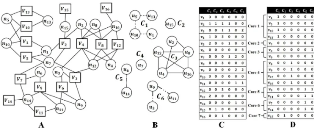
Fig. 1:An example of the coarsening procedure. (a) The sample hypergraph. (b)HCG
usingweighted jaccard index in (3) and similarity thresholds= 0.5. (c) The reduced information system, and (d) Remaining attributes after removing superfluous attributes for clustering thresholdc= 0.5.
The next step is to remove superfluous attributes from ER. A clustering
thresholdc∈[0,1] is defined and the mapping function of (4) is transformed to:
Ff(v, e R) = ( 1, if FR(v,eR) |{e.v,∀e∈E}| >c 0, otherwise. (5)
At this point we have a reduced information systemIf and we use this to find
clusters of vertices using rough set clustering techniques. Using the indiscernibility relation defined in (2), the equivalence relation between vertices (Sect. 3.2), and the mapping functionFfof (5),
U/IND(ER) provides a partitioning of the vertex
setV. The parts are called the cores of the hypergraph. Cores of unit size as well as vertices whoseFf(v, e
R) = 0, ∀eR∈ER are categorised as non–core vertices
and they will be processed after core vertices. The cores are visited one at a time and they are searched locally to find the best matching pairs according to (3). The larger the mean vertex degree in the hypergraph is, the larger denominator we get in (5) and this makes it difficult to choose a clustering threshold. As a result, large mean vertex degrees produce more cores of unit size and this causes the number of vertices that belong to cores to be small compared to|V|.
To maintain a certain compression ratio between two successive levels of the coarsening, we perform a random matching of the non–core vertices. An example of the coarsening procedure is given in Fig. 1.
4.2 Initial Partitioning and Uncoarsening
In the initial partitioning phase, a bipartitioning on the coarsest hypergraphHc
is found using a number of algorithms. An output is selected to be projected back to the original hypergraph: if many outputs fulfill the balancing requirement then the one with lowest cost is chosen else it is the output that comes closest to
Table 1:Tested hypergraphs and their specifications
Hypergraph Description Rows Columns Non-Zeros Structure1
NSC2
CNR–2000 Small web crawl of Italian CNR domain 325,557 325,557 3,216,152 USYM 100,977 AS–22JULY06 Internet routers 22,963 22,963 96,872 SYM 1 CELEGANSNEURAL Neural Network of Nematode C. Elegans 297 297 2,345 USYM 57 NETSCIENCE Co-authorship of scientists in Network Theory 1,589 1,589 5,484 SYM 396 PGPGIANTCOMPO Largest connected component in graph of PGP users 10,680 10,680 48,632 SYM 1 GUPTA1 Linear Programming matrix (A×AT) 31,802 31,802 2,164,210 SYM 1 MARK3JAC120 Jacobian from MULTIMOD Mark3 54,929 54,929 322,483 USYM 1,921 NOTREDAME Barabasi’s web page network of nd.edu 325,729 325,729 929,849 USYM 231,666 PATENTS–MAIN Pajek network: mainNBER US Patent Citations 240,547 240,547 560,943 USYM 240,547 STD1–JAC3 Chemical process simulation 21,982 21,982 1,455,374 USYM 1 COND–MAT–2005 Collaboration network, www.arxiv.org 40,421 40,421 351,382 SYM 1,798
1
NSC stands for the number of strongly connected components.
2
SYM stands for symmetric and USYM stands for unsymmetric.
meeting the balancing requirement. The algorithms used are random partitioning (randomly assign vertices to parts), linear partitioning (linearly assign vertices to parts), and a modification of the FM algorithm [10]. During uncoarsening, we try to refine the quality of the partitioning by moving the vertices across the partition boundary. A vertex is on the boundary if at least one of its incident edges is cut by the bipartitioning. The FM algorithm and its variants have been shown to be successful for the refinement process [8, 16] and we use a modified version of FM orBoundary FM algorithm.
5
Evaluation
We have compared our algorithm (FEHG) withPHG (the Zoltan hypergraph partitioner) [8], hMetis [16], and PaToH [4]. These algorithms achievek-way partitioning by recursive bipartitioning. The evaluated hypergraphs listed in Table 1 are from the University of Florida Sparse Matrix Collection [7]. They are from a variety of applications with different specifications and include both symmetric and non–symmetric instances, and hypergraphs with different numbers of strongly connected components, etc. Each matrix in the table is treated as a hypergraph. We use the column-net model where each row of the matrix corre-sponds to a vertex and each column correcorre-sponds to a hyperedge [8]. The weights of vertices and hyperedges are set to unity. The evaluated tools have different input parameters that can be selected by the user. For our case, we use default settings for the comparison:shmetis is the default partitioner selected forhMetis,PaToH is initialised by settingSBProbTypeparameter toPATOH SUGPARAM DEFAULT, and the coarsening algorithm for PHG is set toagglomerative. All of them use a variation ofFM for the refinement and uncoarsening phase.
FEHG has two input parameters: thesimilarity threshold to constructHCG, and the clustering threshold from (5). The values chosen for these parameters can have a large impact on the quality of the partitioning. We describe how calculate the similarity threshold when the Jaccard Index is used for measuring the similarity between hyperedges.
The Clustering Coefficient (CC) is a graph theory measure determined by the degree to which a node clusters with other nodes of the graph or hypergraph.
Different methods for finding CC in hypergraphs have been proposed [18]. Given a hypergraphH = (V, E), we define CC for a hyperedgee∈E as:
CC(e) = P {e0 ∩e6=∅} 1−(|e|−|1)e|−−|1e∩e0| ·γ(e0) P {v∈e} P {e00.v}γ(e00) ,∀e 0, e00∈E\e, if|e|>1 0, otherwise. (6)
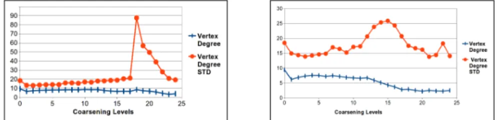
The CC of the hypergraph is calculated as the average CC over all hyperedges. We calculate CC at the start of the algorithm. As the structure of the hypergraph changes at each level of coarsening, we readjust its value instead of recalculation. As proposed in [11] to analyse Facebook social networks and theoretically inves-tigated in [3] on sparse random intersection graphs, the clustering of nodes in hypergraphs is inversely correlated with average vertex degree. Based on this, we readjust CC’s value according to the variation of average vertex degree from one level of the coarsening to the next. Finally, CC value of the hypergraph is set as the similarity threshold at each coarsening level.
Figure 2a depicts the variation of similarity threshold for each coarsening level of a tested graph CNR–2000. Both the readjusted value and the actual value are shown. The readjusted value provides a lower bound for the actual value and it is about 50% of its value from the third iteration onward which is sufficient for feature reduction. In Fig. 2b, the percentage of the edges whose clustering coefficients are at least equal to the similarity threshold along with normalised variation of edge size and its standard deviation (STD) is represented. As the partitioner gets close to the coarsest hypergraph we have small average size of hyperedges (2.09) and small average vertex degrees (2.47) but larger vertex degree standard deviation (14.33); most of the vertices share very few hyperedges so clustering decisions are difficult. As we see, the automatic readjustment still catches the possible similarities. In general we achieve a cut size 50 for CNR–2000.
In our evaluation we found that variation of the similarity threshold has higher impact on the quality of the partitioning than the clustering threshold. The reason is that hyperedges with higher CC value are more likely to cluster with others and they get higher coefficient in (4) and tend to be included in the final reduced information system in (5). This reduces the effects of clustering threshold variations. Therefore, we remove each eR∈ER of unit size (refer to
Sect. 4.1) and we set the clustering threshold to 0 in (5) for the others. For example, edge partitionsC2 andC4 are removed from the table in Fig. 1c. For all tested hypergraphs, the algorithms are each run 20 times and the average and best cut sizes are reported. Simulations are done with 2% imbalance tolerance in (1) and the number of parts are{2,4,8,16,32}. The final imbalance achieved by the algorithms are not reported because the balancing requirement was always met by all algorithms. The simulation results as well as standard deviation from the average cut are reported in Table 2. The latter could be used as a measure of the robustness of the algorithms specifically when they give close partitioning quality. The values are normalised with the best cut generated among all algorithms except the standard deviation. According to the results,FEHG performs very well compared to Zoltan andhMetis and it is competitive with
(a)Similarity Threshold (b)Changevs.edge size and its STD
Fig. 2:(a) Readjustedsimilarity threshold sfor the test hypergraph CNR–2000 accord-ing to (6) compared to its recalculation at each coarsenaccord-ing level. (b) The percentage of the hyperedges whose CC is more thansand comparison to normalised edge size edge and its standard deviation (STD).
Fig. 3:Variation of vertex degree and its standard deviation whenFEHGmakes extra effort for achieving maximum vertex similarity matching vs normal matching
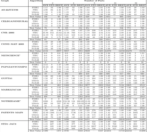
PaToH. For example in Noterdame and Patents-Main, FEHG achieves a superior quality improvement compared toZoltan andhMetis. In another simulation, we investigate whether relying only on a vertex similarity metric is enough to achieve better partition quality. When two vertices are matched, we refer to their similarity degree as the roughness of the match and it is calculated using (3). Matching pairs of vertices with higher similarity degree at each level of coarsening means higher average roughness of the matched vertices in that level. According to the algorithms that investigate vertex similarity metrics, an algorithm would be better if it yields higher average roughness for levels of coarsening compared to the others [21]. Furthermore, the decision about the vertex similarity is made locally in those algorithms without collecting global information. InFEHG, we refer to the average roughness of core vertices as core roughness. We consider two scenarios for our test while we find a pair match for non–core vertices: in the first one, a match is allowed for a non–core vertex if the roughness of the match is at least equal to the core roughness. In the second scenario we allow non–core vertex to be matched to any vertex as long as the roughness of the match is greater than zero. In the first scenario, the emphasis is on finding vertices with higher similarity as is the case for similarity metric based methods and it guarantees higher average roughness compared to the second scenario during levels of coarsening. The test is done on the hypergraphs and the result
Table 2:Quality comparison of the algorithms for different part sizes and imbalance factor 2% with normalised values.
Graph Algorithm Number of Parts
2 4 8 16 32
AVE STD BEST AVE STD BEST AVE STD BEST AVE STD BEST AVE STD BEST
FEHG 1.11 34 1.00 1.02 32 1.00 1.04 25 1.01 1.01 30 1.00 1.01 28 1.03 AS-22JULY06 PHG 2.90 86 2.46 1.77 92 1.56 1.64 78 1.36 1.43 87 1.34 1.37 90 1.32 hMetis 1.34 0 1.95 1.19 7 1.30 1.16 12 1.18 1.04 23 1.06 1.09 27 1.04 PaToH 1.00 4 1.43 1.00 16 1.03 1.00 20 1.00 1.00 37 1.00 1.00 43 1.00 Best Value 136 – 93 355 – 319 629 – 599 1051 – 995 1591 – 1529 FEHG 1.00 2 1.00 1.09 9 1.00 1.10 15 1.06 1.11 16 1.08 1.07 17 1.03 CELEGANSNEURAL PHG 1.07 6 1.00 1.04 8 1.03 1.02 9 1.00 1.06 12 1.00 1.00 18 1.00 hMetis 1.17 0 1.21 1.00 5 1.05 1.00 0 1.04 1.00 2 1.02 1.00 6 1.00 PaToH 1.01 0 1.04 1.00 0 1.06 1.03 0 1.07 1.03 0 1.06 1.05 0 1.05 Best Value 79 – 77 195 – 184 354 – 342 548 – 536 773 – 769 FEHG 1.37 63 1.00 1.71 131 1.07 1.59 226 1.41 1.53 218 1.45 1.63 217 1.51 CNR–2000 PHG 35.88 552 45.62 12.48 760 9.17 5.73 569 4.84 3.54 477 2.98 2.42 530 2.02 hMetis 12.19 74 18.82 8.24 163 8.43 5.08 240 4.71 3.46 238 3.29 2.66 231 2.50 PaToH 1.00 3 1.71 1.00 37 1.00 1.00 48 1.00 1.00 62 1.00 1.00 85 1.00 Best Value 81 – 45 244 – 202 569 – 509 1014 – 911 1927 – 1830 FEHG 1.00 28 1.00 1.00 58 1.00 1.00 87 1.00 1.01 88 1.02 1.01 82 1.00 COND–MAT–2005 PHG 1.17 37 1.17 1.11 84 1.10 1.05 94 1.05 1.03 112 1.03 1.02 105 1.01 hMetis 1.05 14 1.07 1.11 75 1.12 1.11 81 1.12 1.11 129 1.10 1.01 122 1.01 PaToH 1.02 39 1.02 1.03 193 1.03 1.00 98 1.00 1.00 153 1.10 1.00 178 1.00 Best Value 2134 – 2087 5057 – 4951 8609 – 8485 12370 – 12150 16270 – 16150 FEHG 0.0 0 0.0 0.0 0 0.0 2.00 1 1.50 1.50 2 1.00 2.08 2 1.81 NETSCIENCE* PHG 0.0 0 0.0 0.0 0 0.0 1.50 1 1.00 1.40 2 1.00 1.87 2 1.5 hMetis 2.0 0 2.0 5.0 0 5.0 4.22 1 3.50 1.75 0 1.75 1.99 2 1.87 PaToH 0.0 0 0.0 0.0 0 0.0 1.00 0 1.00 1.00 0 1.00 1.00 0 1.00 Best Value 0 – 0 0 – 0 2 – 2 8 – 8 16 – 16 FEHG 2.12 8 1.27 1.00 23 1.00 1.04 18 1.00 1.00 16 1.08 1.00 18 1.00 PGPGIANTCOMPO PHG 13.23 48 1.83 1.44 65 1.04 1.25 45 1.04 1.02 53 1.00 1.08 46 1.00 hMetis 9.7 3 9.61 1.46 11 1.71 1.04 13 1.40 1.31 24 1.40 1.26 25 1.27 PaToH 1.00 0 1.00 1.04 0 1.27 1.00 7 1.04 1.02 2 1.15 1.08 5 1.06 Best Value 18 – 18 242 – 200 419 – 400 695 – 617 956 – 930 FEHG 1.00 60 1.00 1.00 55 1.00 1.00 80 1.00 1.00 115 1.00 1.00 15 1.00 GUPTA1 PHG 1.58 67 1.45 1.31 146 1.24 1.15 204 1.04 1.07 253 1.04 1.09 58 1.05 hMetis 1.73 2 1.82 1.61 10 1.69 1.58 58 1.64 1.60 137 1.57 1.51 643 1.48 PaToH 1.22 32 1.17 1.08 43 1.09 1.04 84 1.05 1.05 95 1.07 1.08 120 1.09 Best Value 486 – 462 1466 – 1384 3077 – 2893 5342 – 5134 8965 – 8519 FEHG 1.01 6 1.01 1.02 18 1.01 1.01 23 1.00 1.00 83 1.00 1.06 132 1.07 MARK3JAC120 PHG 1.00 4 1.01 1.02 15 1.02 1.02 27 1.00 1.00 53 1.00 1.72 106 1.78 hMetis 1.00 13 1.00 1.00 15 1.02 1.00 29 1.00 1.30 217 1.00 4.20 214 1.78 PaToH 1.00 0 1.02 1.00 11 1.00 1.00 17 1.00 1.26 248 1.20 1.00 267 1.00 Best Value 408 – 400 1229 – 1202 2856 – 2835 6317 – 6245 3142 – 2944 FEHG 0 0 0 1.00 9 1.00 1.12 40 1.12 1.09 116 1.03 1.06 119 1.07 NOTREDAME* PHG 4326 0 4326 158.56 124 288.69 13.82 67 16.78 2.09 75 3.06 1.72 78 1.78 hMetis 880 84 707 67.92 65 129.92 10.98 108 12.65 3.36 143 3.37 2.23 129 2.30 Patoh 24 1 22 1.90 8 3.31 1.00 27 1.00 1.00 52 1.00 1.00 62 1.00 Best Value 0 – 0 27 – 13 316 – 259 1577 – 1484 3142 – 2944 FEHG 1.20 180 1.00 1.03 275 1.01 1.05 270 1.03 1.00 327 1.00 1.00 342 1.00 PATENTS–MAIN PHG 12.49 1286 13.19 2.52 1736 2.30 1.79 1749 1.65 1.42 1575 1.38 1.23 1602 1.18 hMetis 2.38 36 2.77 1.16 70 1.24 1.26 115 1.43 1.26 161 1.31 1.21 231 1.22 PaToH 1.00 70 1.02 1.00 145 1.00 1.00 217 1.00 1.00 220 1.00 1.01 306 1.00 Best Value 643 – 528 3490 – 3198 6451 – 6096 11322 – 10640 16927 – 16460 FEHG 1.01 260 1.00 1.00 246 1.03 1.00 424 1.00 1.00 549 1.00 1.00 557 1.00 STD1–JAC3 PHG 1.15 227 1.08 1.16 377 1.10 1.18 748 1.13 1.28 768 1.35 1.33 801 1.29 hMetis 1.05 105 1.00 1.52 1649 1.03 1.54 2057 1.23 1.70 2330 1.53 1.71 2995 1.51 Patoh 1.00 125 1.00 1.08 506 1.00 1.16 700 1.14 1.00 827 1.26 1.30 945 1.29 Best Value 1490 – 1371 3735 – 3333 7616 – 6167 13254 – 11710 22242 – 21200
*When the minimum cut for the average or best cases are zero, the values shown are actual cut values rather than normalised values.
for CNR-2000 is reported in Fig. 3. According to the results, the first scenario causes high fluctuations of vertex degree standard deviations while the second scenario produces a smooth change. We achieve average cuts of 490 and 110 for CNR–2000 for the first and second scenarios, respectively.
The agglomerative clustering ofZoltan andhMetis give 25.54 and 8.89 times worse quality.PaToH also produces good average quality of 81 using absorption clustering using pins and hyperedge clustering. The variations in vertex degree or its standard deviation causes problems for clustering algorithms, making it hard to make good clustering decisions because of the increased conflicts between local and global decisions. Consequently, finding vertices with higher similarity for matching can not be relied on for every hypergraph and it does not always gives a better partitioning cut. In addition, gathering some global information before making clustering decisions can give a major quality improvement and decreases the unexpectedness of the partitioning cut as depicted in Table 2.
6
Conclusions and Future Work
We have proposed a multi–level hypergraph partitioning algorithm based on feature extraction and attribute reduction using rough set clustering techniques. The algorithm clusters hyperedges using different similarity metrics and a simi-larity threshold and tries to removes less important hyperedges. An automated calculation of this similarity threshold is proposed. The hypergraph is then transformed into a reduced information system. Employing the idea of Rough Set clustering, the algorithm calculates the partitioning of the objects in the reduced information system based on indispensability relations and core sets of vertices with globally high similarities. Then cores are searched locally for vertex matchings. Evaluating the algorithm in comparison to the state-of-the-art algorithms has shown improvements in quality of the partitioning for tested hypergraphs. Future work is to implement parallel versions of the algorithm. Using a special distribution of vertices and hyperedges among processors and the ideas of rough set theory, we are focusing on proposing a scalable partitioner.
Acknowledgments
This work is supported by the EU FP7 Marie Curie Initial Training Network “SCALUS — Scaling by means of Ubiquitous Storage” under grant agreement No.238808. We thank the Efficient Computing and Storage Group at Johannes Gutenberg Universit¨at Mainz, Germany for their help and support.
References
[1] C. Aykanat, B. B. Cambazoglu, and B. U¸car. “Multi-level direct K-way hypergraph partitioning with multiple constraints and fixed vertices”. In: Journal of Parallel and Distributed Computing 68.5 (2008), pp. 609–625. [2] J. G. Bazan, M. S. Szczuka, A. Wojna, and M. Wojnarski. “On the evolution
of rough set exploration system”. In:Rough Sets and Current Trends in Computing. Springer. 2004, pp. 592–601.
[3] M. Bloznelis et al. “Degree and clustering coefficient in sparse random intersection graphs”. In: The Annals of Applied Probability 23.3 (2013), pp. 1254–1289.
[4] U. V. Catalyurek and C. Aykanat. “Hypergraph-partitioning-based de-composition for parallel sparse-matrix vector multiplication”. In: IEEE Transactions on Parallel and Distributed Systems 10.7 (1999), pp. 673–693. [5] U. Catalyurek, E. Boman, K. Devine, D. Bozdag, R. Heaphy, and L. Riesen. “Hypergraph-based Dynamic Load Balancing for Adaptive Scientific Com-putations”. In:Parallel and Distributed Processing Symposium (IPDPS’07). 2007, pp. 1–11.
[6] C. Curino, E. Jones, Y. Zhang, and S. Madden. “Schism: A Workload-driven Approach to Database Replication and Partitioning”. In: Proc. VLDB Endow.3.1-2 (2010), pp. 48–57.
[7] T. A. Davis and Y. Hu. “The University of Florida sparse matrix collection”. In:ACM Transactions on Mathematical Software 38.1 (2011), p. 1. [8] K. D. Devine, E. G. Boman, R. T. Heaphy, R. H. Bisseling, and U. V.
Catalyurek. “Parallel Hypergraph Partitioning for Scientific Computing”. In:Proc. of 20th International Parallel and Distributed Processing Sympo-sium (IPDPS’06). IEEE, 2006.
[9] L. Ert¨oz, M. Steinbach, and V. Kumar. “Finding clusters of different sizes, shapes, and densities in noisy, high dimensional data.” In: SDM. SIAM. 2003, pp. 47–58.
[10] C. M. Fiduccia and R. M. Mattheyses. “A linear-time heuristic for improving network partitions”. In: 19th Conference on Design Automation. IEEE. 1982, pp. 175–181.
[11] I. Foudalis, K. Jain, C. Papadimitriou, and M. Sideri. “Modeling Social Networks Through User Background and Behavior”. In: Proceedings of the 8th International Conference on Algorithms and Models for the Web Graph. WAW’11. Atlanta, GA: Springer-Verlag, 2011, pp. 85–102.
[12] M. R. Garey and D. S. Johnson. Computers and intractability. Vol. 29. W. H. Freeman, 2002.
[13] B. Heintz and A. Chandra. “Beyond Graphs: Toward Scalable Hypergraph Analysis Systems”. In: SIGMETRICS Perform. Eval. Rev. 41.4 (2014), pp. 94–97.
[14] B. Hendrickson and T. G. Kolda. “Graph partitioning models for parallel computing”. In: Parallel computing 26.12 (2000), pp. 1519–1534.
[15] T. Hu, C. Liu, Y. Tang, J. Sun, H. Xiong, and S. Y. Sung. “High-dimensional clustering: a clique-based hypergraph partitioning framework”. In: Knowl-edge and information systems 39.1 (2014), pp. 61–88.
[16] G. Karypis, R. Aggarwal, V. Kumar, and S. Shekhar. “Multilevel hyper-graph partitioning: applications in VLSI domain”. In:IEEE Transactions on Very Large Scale Integration (VLSI) Systems 7.1 (1999), pp. 69–79. [17] E. Kayaaslan, A. Pinar, ¨U. C¸ ataly¨urek, and C. Aykanat. “Partitioning
Hypergraphs in Scientific Computing Applications through Vertex Separa-tors on Graphs”. In:SIAM Journal on Scientific Computing 34.2 (2012), A970–A992.
[18] M. Latapy, C. Magnien, and N. D. Vecchio. “Basic notions for the analysis of large two-mode networks”. In: Social Networks 30.1 (2008), pp. 31–48. [19] Z. Pawlak.Rough Sets: Theoretical Aspects of Reasoning About Data.
Nor-well, MA, USA: Kluwer Academic Publishers, 1991.
[20] Z. Tian, T. Hwang, and R. Kuang. “A hypergraph-based learning algorithm for classifying gene expression and arrayCGH data with prior knowledge”. In:Bioinformatics 25.21 (2009), pp. 2831–2838.
[21] A. Trifunovic. “Parallel algorithms for hypergraph partitioning”. PhD thesis. University of London, 2006.
[22] B. Vastenhouw and R. H. Bisseling. “A two-dimensional data distribution method for parallel sparse matrix-vector multiplication”. In: SIAM review 47.1 (2005), pp. 67–95.