Roman Denysiuk
outubro de 2013
UMinho|20
13
Evolutionary Multiobjective Optimization:
Review, Algorithms, and Applications
Escola de Engenharia
R oman Den ysiuk Ev olutionar y Multiobjective Op timization: R e vie w , Algorit hms, and ApplicationsPrograma Doutoral em Engenharia Industrial e Sistemas
Trabalho realizado sob a orientação do
Professor Doutor Lino Costa
e da
Professora Doutora Isabel Espírito Santo
Roman Denysiuk
outubro de 2013
Evolutionary Multiobjective Optimization:
Review, Algorithms, and Applications
Escola de Engenharia
Abstract
Many mathematical problems arising from diverse fields of human activity can be formu-lated as optimization problems. The majority of real-world optimization problems involve several and conflicting objectives. Such problems are called multiobjective optimization problems (MOPs). The presence of multiple conflicting objectives that have to be simul-taneously optimized gives rise to a set of trade-off solutions, known as the Pareto optimal set. Since this set of solutions is crucial for effective decision-making, which generally aims to improve the human condition, the availability of efficient optimization methods becomes indispensable.
Recently, evolutionary algorithms (EAs) have become popular and successful in approx-imating the Pareto set. The population-based nature is the main feature that makes them especially attractive for dealing with MOPs. Due to the presence of two search spaces, operators able to efficiently perform the search in both the decision and objective spaces are required. Despite the wide variety of existing methods, a lot of open research issues in the design of multiobjective evolutionary algorithms (MOEAs) remains.
This thesis investigates the use of evolutionary algorithms for solving multiobjective optimization problems. Innovative algorithms are developed studying new techniques for performing the search either in the decision or the objective space. Concerning the search in the decision space, the focus is on the combinations of traditional and evolutionary optimization methods. An issue related to the search in the objective space is studied in the context of many-objective optimization.
Application of evolutionary algorithms is addressed solving two different real-world problems, which are modeled using multiobjective approaches. The problems arise from the mathematical modelling of the dengue disease transmission and a wastewater treatment plant design. The obtained results clearly show that multiobjective modelling is an effective approach. The success in solving these challenging optimization problems highlights the practical relevance and robustness of the developed algorithms.
Resumo
Muitos problemas matem´aticos que surgem nas diversas ´areas da actividade humana po-dem ser formulados como problemas de otimiza¸c˜ao. A maioria dos problemas do mundo real envolve v´arios objetivos conflituosos. Tais problemas chamam-se problemas de otimiza¸c˜ao multiobjetivo. A presen¸ca de v´arios objetivos conflituosos, que tˆem de ser otimizados em simultˆaneo, d´a origem a um conjunto de solu¸c˜oes de compromisso, conhecido como con-junto de solu¸c˜oes ´otimas de Pareto. Uma vez que este conjunto de solu¸c˜oes ´e fundamental para uma tomada de decis˜ao eficaz, cujo objetivo em geral ´e melhorar a condi¸c˜ao humana, o desenvolvimento de m´etodos de otimiza¸c˜ao eficientes torna-se indispens´avel.
Recentemente, os algoritmos evolucion´arios tornaram-se populares e bem sucedidos na aproxima¸c˜ao do conjunto de Pareto. A natureza populacional ´e a principal caracter´ıstica que os torna especialmente atraentes para lidar com problemas de otimiza¸c˜ao multiob-jetivo. Devido `a presen¸ca de dois espa¸cos de procura, operadores capazes de realizar a procura de forma eficiente, tanto no espa¸co de decis˜ao como no espa¸co dos objetivos, s˜ao necess´arios. Apesar da grande variedade de m´etodos existentes, v´arias quest˜oes de inves-tiga¸c˜ao permanecem em aberto na ´area do desenvolvimento de algoritmos evolucion´arios multiobjetivo.
Esta tese investiga o uso de algoritmos evolucion´arios para a resolu¸c˜ao de problemas de otimiza¸c˜ao multiobjetivo. S˜ao desenvolvidos algoritmos inovadores que estudam novas t´ecnicas de procura, quer no espa¸co de decis˜ao, quer no espa¸co dos objetivos. No que diz re-speito `a procura no espa¸co de decis˜ao, o foco est´a na combina¸c˜ao de m´etodos de otimiza¸c˜ao tradicionais com algoritmos evolucion´arios. A quest˜ao relacionada com a procura no espa¸co dos objetivos ´e desenvolvida no contexto da otimiza¸c˜ao com muitos objetivos.
A aplica¸c˜ao dos algoritmos evolucion´arios ´e abordada resolvendo dois problemas reais, que s˜ao modelados utilizando abordagens multiobjetivo. Os problemas resultam da mod-ela¸c˜ao matem´atica da transmiss˜ao da doen¸ca do dengue e do desenho ´otimo de esta¸c˜oes de tratamento de ´aguas residuais. O sucesso na resolu¸c˜ao destes problemas de otimiza¸c˜ao constitui um desafio e destaca a relevˆancia pr´atica e robustez dos algoritmos desenvolvidos.
Acknowledgments
I would like to thank my advisors Lino Costa and Isabel Esp´ırito Santo for introducing me to multiobjective optimization, giving me the opportunity to do postgraduate research, and helping me through this time. I am also thankful to Teresa Monteiro for believing in me and helping me. I am grateful to my parents Tetyana and Vitaliy, who made my education possible. Finally, I would like to thank my sisters Hanna and Oksana for encouragement and support.
Abstract i
Acknowledgments v
List of Tables xv
List of Figures xvii
List of Acronyms xxi
1 Introduction 1
1.1 Motivation . . . 1
1.2 Outline of the Thesis . . . 4
1.3 Contributions . . . 5
I
Review
7
2 Multiobjective Optimization Background 9 2.1 Introduction . . . 9 2.2 General Concepts . . . 10 2.3 Optimality Conditions . . . 17 2.3.1 First-Order Conditions . . . 18 2.3.2 Second-Order Conditions . . . 19 ix2.4 Summary . . . 20
3 Multiobjective Optimization Algorithms 23 3.1 Introduction . . . 23
3.2 Classical Methods . . . 25
3.2.1 Weighted Sum Method . . . 25
3.2.2 -Constraint Method . . . 27
3.2.3 Weighted Metric Methods . . . 28
3.2.4 Normal Boundary Intersection Method . . . 30
3.2.5 Normal Constraint Method . . . 32
3.2.6 Timmel’s Method . . . 34
3.3 Evolutionary Multiobjective Optimization Algorithms . . . 36
3.3.1 Genetic Algorithm-Based Approaches . . . 36
3.3.2 Evolution Strategy-Based Approaches . . . 41
3.3.3 Differential Evolution-Based Approaches . . . 44
3.3.4 Particle Swarm Optimization-Based Approaches . . . 47
3.3.5 Scatter Search-Based Approaches . . . 49
3.3.6 Simulated Annealing-Based Approaches . . . 51
3.3.7 Covariance Matrix Adaptation Evolution Strategy-Based Approaches 54 3.3.8 Estimation of Distribution Algorithm-Based Approaches . . . 57
3.3.9 Multiobjective Evolutionary Algorithm Based on Decomposition . . 58
3.4 Evolutionary Many-Objective Optimization Algorithms . . . 63
3.4.1 Selection Pressure Enhancement . . . 64
3.4.2 Different Fitness Assignment Schemes . . . 68
3.4.3 Use of Preference Information . . . 74
3.4.4 Dimensionality Reduction . . . 76
4 Performance Assessment of Multiobjective Optimization Algorithms 85
4.1 Introduction . . . 85
4.2 Benchmark Problems . . . 87
4.3 Quality Indicators . . . 90
4.3.1 Indicators Evaluating Convergence . . . 91
4.3.2 Indicators Evaluating Diversity . . . 93
4.3.3 Indicators Evaluating Convergence and Diversity . . . 98
4.4 Statistical Comparison . . . 101 4.4.1 Attainment Surface . . . 101 4.4.2 Statistical Testing . . . 103 4.4.3 Performance Profiles . . . 105 4.5 Summary . . . 106
II
Algorithms
109
5 Hybrid Genetic Pattern Search Augmented Lagrangian Algorithm 111 5.1 Introduction . . . 1115.2 HGPSAL . . . 112
5.2.1 Augmented Lagrangian . . . 112
5.2.2 Genetic Algorithm . . . 115
5.2.3 Hooke and Jeeves . . . 117
5.2.4 Performance Assessment . . . 118
5.3 MO-HGPSAL . . . 125
5.3.1 Performance Assessment . . . 126
5.4 Summary . . . 130
6 Descent Directions-Guided Multiobjective Algorithm 131 6.1 Introduction . . . 131
6.2.1 Initialize Procedure . . . 133
6.2.2 Update Search Matrix Procedure . . . 134
6.2.3 Update Step Size Procedure . . . 140
6.2.4 Parent Selection Procedure . . . 141
6.2.5 Mutation Procedure . . . 142
6.2.6 Environmental Selection Procedure . . . 142
6.3 Performance Assessment . . . 143
6.3.1 Preliminary Experiments . . . 144
6.3.2 Intermediate Summary . . . 146
6.3.3 Further Experiments . . . 147
6.4 Summary . . . 161
7 Generalized Descent Directions-Guided Multiobjective Algorithm 163 7.1 Introduction . . . 163
7.2 DDMOA2 . . . 164
7.2.1 Initialize Procedure . . . 165
7.2.2 Leader Selection Procedure . . . 165
7.2.3 Update Search Matrix Procedure . . . 166
7.2.4 Update Step Size Procedure . . . 167
7.2.5 Parent Selection Procedure . . . 168
7.2.6 Mutation Procedure . . . 169
7.2.7 Environmental Selection Procedure . . . 169
7.3 Performance Assessment . . . 170
7.3.1 Preliminary Experiments . . . 170
7.3.2 Intermediate Summary . . . 177
7.3.3 Further Experiments . . . 178
8 Many-Objective Optimization using DEMR 191
8.1 Introduction . . . 191
8.2 DEMR for Multiobjective Optimization . . . 192
8.2.1 NSDEMR . . . 192
8.2.2 Performance Assessment . . . 195
8.2.3 Intermediate Summary . . . 197
8.3 IGD-Based Selection for Evolutionary Many-Objective Optimization . . . . 198
8.3.1 EMyO-IGD . . . 198
8.3.2 Performance Assessment . . . 200
8.3.3 Intermediate Summary . . . 208
8.4 Clustering-Based Selection for Evolutionary Many-Objective Optimization 209 8.4.1 EMyO-C . . . 209
8.4.2 Performance Assessment . . . 211
8.5 Summary . . . 214
III
Applications
217
9 Dengue Disease Transmission 219 9.1 Disease Background . . . 2199.2 ODE SEIR+ASEI Model with Insecticide Control . . . 222
9.3 Multiobjective Approach . . . 226
9.4 Summary . . . 233
10 Wastewater Treatment Plant Design 235 10.1 Activated Sludge System . . . 235
10.2 Mathematical Model . . . 237
10.3 Multiobjective Approach . . . 250
10.4 Many-Objective Approach . . . 255
11 Conclusions 261 11.1 Conclusions . . . 261 11.2 Future Perspectives . . . 265
Bibliography 267
5.1 Test problems. . . 119
5.2 Augmented Lagrangian parameters. . . 120
5.3 Genetic algorithm parameters. . . 120
5.4 Median values of IGD. . . 127
6.1 Median values of the epsilon indicator after 30 runs. . . 150
6.2 Median values of the hypervolume indicator after 30 runs. . . 151
7.1 Statistical comparison in terms of IGD. . . 172
7.2 Statistical comparison in terms of IIGD. . . 172
7.3 Comparison in terms of GD. . . 184
7.4 Comparison in terms of IGD. . . 184
8.1 Parameter settings for the algorithms. . . 201
8.2 Statistical comparison in terms of the hypervolume. . . 206
8.3 Statistical comparison in terms of IGD. . . 207
10.1 Optimal values for the most important variables obtained using multiobjective approach. . . 254
10.2 Optimal values for the most important variables obtained using many-objective approach. . . 257
2.1 Representation of the decision space and the corresponding objective space. 11
2.2 Representation of solutions in two different spaces. . . 12
2.3 Representation of the additive-dominance. . . 13
2.4 Representation of the Pareto optimal front. . . 14
2.5 Representation of some special points in multiobjective optimization. . . . 16
3.1 Representation of the weighted sum method. . . 26
3.2 Representation of the -constraint method. . . 27
3.3 Representation of the weighted metric method. . . 29
3.4 Representation of the normal boundary intersection method. . . 31
3.5 Pareto optimal solutions not obtainable using the NBI method. . . 32
3.6 Representation of the NC method. . . 34
3.7 Representation of Timmel’s method. . . 35
3.8 Average percentage of nondominated vectors among 300 randomly generated vectors in the m-dimensional unit hypercube. . . 64
4.1 Performance produced by two algorithms on a same problem. . . 86
4.2 Attainment surfaces and lines of intersection. . . 102
5.1 Performance profiles onfavg and nf evalavg for version 1. . . 121
5.2 Performance profiles onfavg and nf evalavg fors = min(200,10n). . . 122
5.3 Boxplots for different population sizes (problem g02). . . 123 xvii
5.4 Performance profiles onfbest and fmedian. . . 124
5.5 Performance profiles on the best and median values of IGD. . . 127
5.6 Performance of MO-HGPSAL on the ZDT test suite. . . 129
6.1 Representation of the working principle of updateSearchMatrix procedure in the objective space. . . 136
6.2 Representation of the working principle of localSearchprocedure. . . 139
6.3 Step size adaptation. . . 140
6.4 Performance profiles on the median values of quality indicators. . . 145
6.5 Performance of DDMOA on DTLZ1 and DTLZ3 using 10,000 evaluations. 146 6.6 Computation of descent directions for leaders. . . 148
6.7 Performance profiles on the median values of quality indicators. . . 149
6.8 Performance of DDMOA on the ZDT test suite. . . 153
6.9 Performance of DDMOA on the two-objective DTLZ test suite. . . 155
6.10 Performance of DDMOA on the three-objective DTLZ test suite. . . 156
6.11 Performance of DDMOA on the two-objective WFG test suite. . . 158
6.12 Performance of DDMOA on the three-objective WFG test suite. . . 160
7.1 Performance profiles on the median values of quality indicators. . . 171
7.2 Performance of DDMOA2 on the two-objective WFG test suite. . . 175
7.3 Performance of DDMOA2 on the three-objective WFG test suite. . . 177
7.4 Computation of descent directions. . . 179
7.5 Performance comparison of DDMOA2, IBEA, and MOEA/D on the DTLZ test suite. . . 182
7.6 Performance profiles on the median values of quality indicators. . . 183
7.7 Performance of DDMOA2 on the two-objective DTLZ test suite. . . 186
7.8 Performance of DDMOA2 on the three-objective DTLZ test suite. . . 187
7.9 Performance analysis of DDMOA and DDMOA2. . . 188
8.2 Evolution of IGD during the generations. . . 196
8.3 Comparison of NSDE and NSDEMR in terms of IGD. . . 197
8.4 Performance comparison of EMyO-IGD, MOEA/D, IBEA, SMPSO, and GDE3 on the DTLZ1-4 test problems. . . 203
8.5 Performance of EMyO-IGD (left), IBEA (middle), SMPSO (right) on the two and three-objective DTLZ1 and DTLZ3 test problems. . . 204
8.6 Performance profiles on the median values of IGD. . . 208
8.7 Performance comparison of EMyO-C, EMyO-IGD, and IBEA on the DTLZ1-3,7 test problems. . . 212
8.8 Distribution of the proximity indicator on DTLZ2 for EMyO-C. . . 214
9.1 Mosquito Aedes aegypti. . . 220
9.2 Life cycle of Aedes aegypti. . . 221
9.3 Trade-off curves obtained by six different algorithms. . . 228
9.4 Performance comparison of the algorithms in terms of the hypervolume on the dengue transmission model. . . 229
9.5 Mapping of uniformly sampled points in the decision space into the objective space defined by the dengue transmission model. . . 230
9.6 Trade-off curve for the infected population and the control. . . 231
9.7 Different scenarios of the dengue epidemic. . . 232
10.1 Schematic representation of a typical WWTP . . . 236
10.2 Schematic representation of the activated sludge system. . . 236
10.3 Typical solids concentration-depth profile adopted by the ATV design procedure. . . 244
10.4 Solids balance around the settler layers according to the double exponential model. . . 246
10.5 Trade-off curve for the total cost and quality index. . . 253 10.6 Trade-off curves obtained using multiobjective and many-objective approaches.258
AbYSS archive-based hybrid scatter search
AMOSA archived multiobjective simulated annealing ASMactivated sludge model
BSM benchmark simulation model
CEC congress on evolutionary computation
CMA-ES covariance matrix adaptation evolution strategy CMX center of mass crossover
C-PCA correntropy principal component analysis CSTR completely stirred tank reactor
DDMOA descent directions-guided multiobjective algorithm
DDMOA2 generalized descent directions-guided multiobjective algorithm DE differential evolution
DEMR differential evolution with mutation restriction DF dengue fever
DHF dengue hemorrhagic fever DRA dynamical resource allocation DTLZ Deb-Thiele-Laumanns-Zitzler EA evolutionary algorithm
EDA estimation of distribution algorithm EMOevolutionary multiobjective optimization EMyO evolutionary many-objective optimization
EMyO-C evolutionary many-objective optimization algorithm with clustering-based selection
EMyO-IGD evolutionary many-objective optimization algorithm with inverted generational distance-based selection
ER external repository ES evolution strategy
ESP evolution strategy with probabilistic mutation GA genetic algorithm
GAAL genetic algorithm with augmented Lagrangian
GD generational distance
GDEgeneralized differential evolution
HGPSAL hybrid genetic pattern search augmented Lagrangian algorithm HJ Hooke and Jeeves
HJAL Hooke and Jeeves with augmented Lagrangian
HypE hypervolume estimation algorithm IBEA indicator-based evolutionary algorithm IGD inverted generational distance
jMetal metaheuristic algorithms in Java LH Latin hypercube
MEES multiobjective elitist evolution strategy
MMEA probabilistic model-based multiobjective evolutionary algorithm MO multiobjective optimization
MO-CMA-ES multiobjective covariance matrix adaptation evolution strategy MOEA multiobjective evolutionary algorithm
MOEA/D multiobjective evolutionary algorithm based on decomposition MOGA multiobjective genetic algorithm
MO-HGPSAL multiobjective hybrid genetic pattern search augmented Lagrangian algorithm
algorithm with normal boundary intersection method
MO-HGPSALNC multiobjective hybrid genetic pattern search augmented Lagrangian
algorithm with normal constraint method
MO-NSGA-II reference-point based many-objective nondominated sorting genetic algorithm
MOP multiobjective optimization problem
MOPSO multiobjective particle swarm optimization MOSA multiobjective simulated annealing
MSOPS multiple single objective Pareto sampling MVU maximum variance unfolding
NBInormal boundary intersection NC normal constraint
NSDE nondominated sorting differential evolution
NSDEMR nondominated sorting differential evolution with mutation restriction NSGA nondominated sorting genetic algorithm
NSGA-II elitist nondominated sorting genetic algorithm OC optimal control
ODE SEIR+ASEI ordinary differential equations susceptible exposed infected resistant + aquatic susceptible exposed infected
PAES Pareto-archived evolution strategy PCAprincipal component analysis
PCSEA Pareto corner search evolutionary algorithm PDE Pareto differential evolution
PF Pareto optimal front
PISA a platform and programming language independent interface for search algorithms PS Pareto optimal set
PSO particle swarm optimization PWWF peak wet weather flow
SA simulated annealing
SBX simulated binary crossover
SMPSO speed-constrained multiobjective particle swarm optimization SMS-EMOA S metric selection evolutionary multiobjective algorithm SOD-CNT sub-objective dominance count procedure
SOP single-objective optimization problem SP secondary population
SPEA strength Pareto evolutionary algorithm SPX simplex crossover
SS scatter search
VEGAvector evaluation genetic algorithm WFG Walking Fish Group
WHO World Health Organization WWTP wastewater treatment plant ZDT Zitzler-Deb-Thiele
Introduction
1.1
Motivation
An optimization problem can be simply described as the problem of finding the best solu-tion from all feasible solusolu-tions. Such problems do not only occur in science and engineering fields but also in the decision-making, which is an integral part of daily life. As an example, consider a task of buying a car. The buyer seeks to purchase the car that best meets his preferences, given a set of restrictions (e.g. a limited budget).
If only one criterion is considered, the given decision-making problem can be formulated as a single-objective optimization problem (e.g., the only concern is the car price, so the buyer, like any customer, seeks to minimize the cost of purchase). In this case, the existence of a single solution (car) that meets buyer requirements is quite evident (it is possible to find a car at the lowest price). However, in many real-world problems there are several and often conflicting objectives that have to be simultaneously considered. The optimization problems with more than one objective function are commonly known as multiobjective optimization problems.
In our example, suppose the buyer likes rapid sport cars with powerful engines, but also wants to minimize the cost of his purchase. So the buyer’s objectives can be determined as follows: on one hand, the buyer seeks to maximize the car engine power when selecting the
car; on the other hand, the buyer seeks to make a purchase at the lowest possible cost. In his search for a new car, the buyer remarks that a rapid sport car can be bought at a high cost, but when sacrificing engine power he can spend much less money for the purchase. Moreover, considering two cars with the same characteristics it is obvious that a car at the lower cost is preferable; or, from the equally priced cars, the one with a more powerful engine is preferable. Discarding unpreferable options the buyer reduces the set of possible alternatives. Eventually, he ends up with a set of cars where a gain in price does not occur without a loss in engine power. Since none of these found alternatives can be considered to be superior than other in this set, they all are optimal. This set represents different trade-offs between the two criteria (price and engine power). To select a final single alternative from the obtained optimal set, further preference information is required.
Although a multiobjective optimization is basically an optimization process, there are fundamental differences between single-objective and multiobjective optimization. In the case of single-objective optimization, one seeks to find a single optimal solution. Since minimization is often assumed, an optimal solution means a solution with the minimum value of the given objective function. On the other hand, in multiobjective optimization (MO) there is no generally accepted definition of optimum as it is in single-objective optimization.
When several objectives are optimized at the same time, the search space becomes partially ordered. As a consequence, there is no longer a single optimal solution but a set of optimal solutions. This set contains equally important solutions that represent different trade-offs between the given objectives. This set is generally known as the Pareto optimal set, or Pareto set (PS) for short. Approximating the Pareto set is the main goal in multiobjective optimization. However, achieving this goal is not an easy task. The obtained solutions that aim to approximate the Pareto set must be as close as possible to the true Pareto set. On the other hand, as many as possible solutions must be found. Since from the practical point of view usually it is not possible to generate the whole Pareto set, the generated set of solutions must cover the entire Pareto set and be as diverse as possible. Due to the existence of two different and somewhat conflicting goals – the convergence and
diversity – the task of approximating the Pareto set is multiobjective in nature. The first goal is similar to the optimality goal in single-objective optimization. The second goal is specific to multiobjective optimization.
Furthermore, since a multiobjective optimization problem consists of different objec-tives, it inherits all properties of its single-objective functions. There are several properties of objective functions that can make even single-objective optimization difficult, namely, multimodality, high-dimensionality, non-separability, deceptiveness, etc. Thus, a multiob-jective problem possesses all these difficulties in the decision space. At the same time, the presence of multiple conflicting objectives adds additional complexity requiring to perform the search in the objective space as well. Two search spaces and two goals of approxi-mating optimal solutions constitute the fundamental differences between single-objective and multiobjective optimization. In general, they make multiobjective optimization more difficult than single-objective optimization.
Algorithms for solving multiobjective optimization problems must be able to success-fully deal with all of the aforementioned difficulties. They must be able to efficiently explore the search space and find a set of optimal solutions. Mechanisms for providing the convergence to the Pareto optimal region and for maintaining a diversity of obtained solutions must be implemented to an algorithm.
The present thesis addresses multiobjective optimization using evolutionary algorithms. As their single-objective counterparts, multiobjective evolutionary algorithms mimic the principles of natural evolution to perform the search. Due to their ability to simultane-ously deal with a set of candidate solutions and to approximate the Pareto set in a single simulation run, MOEAs became especially attractive for solving multiobjective problems. During the last two decades, they have been successfully applied to solve many real-world multiobjective optimization problems, thereby highlighting their robustness. However, growing complexity of problems emerging in different fields of human activity such as science, engineering, business and medicine, among others, provides new challenges and requires powerful tools for solving these problems. This thesis explores the methodology of evolutionary multiobjective optimization (EMO) and aims to promote this area of research.
1.2
Outline of the Thesis
As the title suggests, the present thesis consists of three major parts: review, algorithms, and applications. Each part comprises a specific aspect of evolutionary multiobjective optimization addressed in this thesis.
Chapter 2 provides the definitions and essential background necessary for the work on multiobjective optimization presented in the following chapters.
Chapter 3 reviews a number of approaches developed for dealing with multiobjective optimization problems. The review includes classical methods and evolutionary algorithms. Additionally, EMO algorithms designed specifically for handling many-objective problems are discussed.
Chapter 4 addresses the issue of performance assessment of multiobjective optimization algorithms. In particular, discussions of the existing test suites, unary quality indicators, and statistical comparison methods used for the performance assessment of multiobjective optimizers are presented. Some of presented techniques are used throughout the thesis for the performance evaluation of the herein proposed algorithms.
Chapter 5 introduces a hybrid approach for constrained single-objective optimization. This approach combines a genetic algorithm with a pattern search method, within an aug-mented Lagrangian framework for constraint handling. After evaluating its performance on a set of constrained single-objective problems, this technique is extended to deal with multiobjective problems.
Chapter 6 suggests a hybrid multiobjective evolutionary algorithm termed descent directions-guided multiobjective algorithm (DDMOA). DDMOA borrows the idea of gener-ating new candidate solutions from Timmel’s method. The proposed framework combines paradigms of classical methods and evolutionary algorithms.
Chapter 7 presents a generalized descent directions-guided multiobjective algorithm (DDMOA2). The convergence property of the original algorithm is improved by allowing all the solutions to participate in the reproduction process. Also, the algorithm is extended for handling many-objective problems by introducing the scalarizing fitness assignment into
the selection process.
Chapter 8 focuses on many-objective optimization. Differential evolution with modified reproduction operator is used as the basis. Two different selection schemes able to guide the search in a high dimensional objective space are proposed.
Chapter 9 reports on applications of EMO algorithms to solve the problem arising from a mathematical modelling of the dengue disease transmission. The performance comparison of different algorithms is carried out on this problem. The obtained trade-off solutions are presented, and different scenarios of the dengue epidemic are discussed.
Chapter 10 considers the problem of finding optimal values of the state variables in a wastewater treatment plant design. Different modelling methodologies, consisting in defining and simultaneously optimizing several objectives, are addressed. The discussion of the obtained results and the analysis of the used approaches to find optimal values are presented.
Chapter 11 concludes the work and discusses some possible future research.
1.3
Contributions
The main contributions of this thesis are:
• A contemporary state-of-the-art of multiobjective optimization. The review con-siders different issues related to multiobjective optimization, including theoretical background, classical methods, evolutionary algorithms, and performance assessment of multiobjective optimizers. The main focus is on multiobjective evolutionary al-gorithms, being their discussion is organized according to reproduction operators. Additional emphasis is put on algorithms designed to deal with many-objective prob-lems.
• A new hybrid evolutionary algorithm [35, 150]. The proposed approach combines a genetic algorithm with a pattern search method, within an augmented Lagrangian
framework for handling constrained problems. The approach is extended to multi-objective optimization adopting frameworks of classical methods for multimulti-objective optimization.
• A new local search based approach for multiobjective optimization [52, 53, 55]. The approach adopts the idea of generating new candidate solutions from Timmel’s method. A local search procedure is introduced to overcome some limitations and to extend its applicability to multiobjective problems with nondifferentiable objective functions. There are two versions of the proposed approach. The first proposal is simpler, yet a viable one. Inspired by promising results of the first version, a gener-alized approach has been developed, resulting in a highly competitive multiobjective optimization algorithm.
• New selection schemes for evolutionary many-objective optimization [54]. Two dif-ferent selection schemes are studied using difdif-ferential evolution with an improved variation operator. The first scheme is indicator-based. It incorporates the inverted generational distance indicator in the selection process. The second scheme aims to provide more flexible and self-adaptive approach. It uses clustering procedure and calculates distances to a reference point to select a representative within each cluster.
• The application of MOEAs to find an optimal control in the mathematical model of the dengue disease transmission. The problem is modeled using a multiobjective approach, which after discretization of the involved system of eight differential equa-tions results in a challenging large-scale optimization problem. The performance of several state-of-the-art EMO algorithms on this real-world problem is also studied.
• The application of the developed algorithms to solve a multiobjective problem aris-ing from a wastewater treatment plant design optimization. Different modelling methodologies to find optimal values of the decision variables in the WWTP design are considered.
Review
Multiobjective Optimization
Background
2.1
Introduction
As the name suggests, a multiobjective optimization problem is an optimization problem that deals with more than one objective. It is quite evident that the majority of practical decision-making and optimization problems in science and engineering possess a number of different usually conflicting objectives. In the past, because of a lack of suitable approaches these problems have been mostly solved as single-objective optimization problems (SOPs). The present chapter introduces the basic concepts of multiobjective optimization and the notation used throughout this thesis. The concepts provided in this chapter are nec-essary for understanding the principles and particularities of multiobjective optimization. Furthermore, the established background is essential for developing efficient approaches to deal with multiobjective optimization problems, which will be described later in this thesis. Thus, a formal definition and some basic concepts in multiobjective optimization are presented in Section 2.2. Furthermore, optimality conditions for any solution to be optimal in the presence of multiple objectives are discussed in Section 2.3.
2.2
General Concepts
A multiobjective optimization problem with m objectives andn decision variables can be formulated mathematically as follows:
minimize: f(x) = (f1(x), . . . , fm(x))T
subject to: gi(x)≤0 i∈ {1, . . . , p}
hj(x) = 0 j ∈ {1, . . . , q}
x∈Ω
(2.2.1)
wherexis the decision vector, Ω⊆Rnand Ω ={x∈
Rn|l≤x≤u},g(x) is the vector of
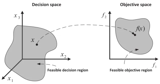
inequality constraints, h(x) is the vector of equality constraints, land uare the lower and upper bounds of the decision variables, respectively, andf(x) is the objective vector defined in the objective space Rm. Minimization is assumed throughout the thesis without loss of generality. From (2.2.1), it can be seen that there are two different spaces. Each solution in the decision space maps uniquely to the objective space. However, the inverse mapping may be non-unique. The mapping, which is performed by a function f :Rn 7→
Rm, takes
place between the n-dimensional decision space and the m-dimensional objective space. Figure 2.1 illustrates the representation of these two spaces and a mapping between them. In (2.2.1), the statement “minimize” means that the goal is to minimize all objective functions simultaneously. If there is no conflict between objectives, then a solution can be found where every objective function achieves its optimum. However, it is a trivial case which is unlikely to be encountered in practice. Another particular case arises whenm= 1. In this case, the problem formulated in (2.2.1) is a single-objective optimization problem. In the following, it is assumed that a problem defined in (2.2.1) does not have a single solution and the number of objectives is not less than two. This means that the objectives are conflicting or at least partly conflicting. Therefore, the presence of multiple conflicting objectives gives rise to a set of optimal solutions, instead of a single optimal solution. This set represents different trade-offs between objectives, and, in the absence of any further information, none of these solutions can be said to be better than other.
1
f
2f
2x
3x
1x
Decision space Objective space
x
)
(
x
f
Feasible decision region Feasible objective region
Figure 2.1: Representation of the decision space and the corresponding objective space.
concept of the Pareto dominance.
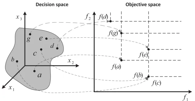
Definition 2.2.1 (Pareto dominance). A vector u = (u1, . . . , uk) is said to dominate a
vector v = (v1, . . . , vk) if and only if:
∀i∈ {1, . . . , k}:ui ≤vi ∧ ∃j ∈ {1, . . . , k}:uj < vj.
Thus, in the context of multiobjective optimization, the following preference relations on the feasible set in the decision space are defined on the basis of the associated objective vectors.
Definition 2.2.2 (weak dominance). Given two solutions a and b from Ω, a solution a
is said to weakly dominate a solution b (denoted by ab) if:
∀i∈ {1, . . . , m}:fi(a)≤fi(b).
Definition 2.2.3 (dominance). Given two solutions a and b from Ω, a solution a is said to dominate a solution b (denoted by a≺b) if:
1
f
2f
2x
3x
1x
Decision space Objective space
a
f
(
a
)
b
c
d
e
g
)
(
b
f
)
(
c
f
)
(
d
f
)
(
e
f
)
(
g
f
Figure 2.2: Representation of solutions in two different spaces.
Definition 2.2.4 (strict dominance). Given two solutions a and b from Ω, a solution a
is said to strictly dominate a solution b (denoted by a≺≺b) if:
∀i∈ {1, . . . , m}:fi(a)< fi(b).
Definition 2.2.5 (incomparability). Given two solutions a and b from Ω, a solution a is said to be incomparable to a solution b (denoted by akb) if:
a b ∧ ba.
Definition 2.2.6 (indifference). Given two solutions a and b from Ω, a solutiona is said to be indifferent (or equivalent) to a solution b (denoted by a≡b) if:
a b ∧ ba.
Figure 2.2 shows a set of solutions {a,b,c,d,e,g} and their image in the objective space. From the figure, it can be seen that a≺≺e,b ≺e,b ≡c, akd, and so on.
The above presented preference relations are also defined on the objective space. How-ever, the indifference relation actually only makes sense with regard to the decision space,
1
f
2f
2x
3x
1x
Decision space Objective space
a
f
(
a
)
b
)
(
b
f
H
)
(
a
f
Figure 2.3: Representation of the additive -dominance.
as in the objective space, it simply means equality. In addition, another widely used pref-erence relation, called-dominance, is defined. Under-dominance, the conditions required for one solution to dominate another are relaxed.
Definition 2.2.7 (multiplicative -dominance). Given two solutions a and b from Ω, a solution a is said to -dominate a solution b (denoted by a b) if for a given :
∀i∈ {1, . . . , m}: (1−)fi(a)≤fi(b).
Definition 2.2.8 (additive-dominance). Given two solutions a andb from Ω, a solution
a is said to -dominate a solution b (denoted by a b) if for a given :
∀i∈ {1, . . . , m}:fi(a)−≤fi(b).
An illustration of the additive-dominance in the biobjective case is shown in Figure 2.3. As we can see, solution a and solution b are incomparable (akb). The region that is -dominated by solution a is composed of the area that would normally be dominated by a plus the areas that would otherwise be nondominated with respect toa or would in fact
1
f
2f
2x
3x
1x
Decision space Objective space
*
x
)
(
x
f
Pareto optimal frontFigure 2.4: Representation of the Pareto optimal front.
dominate a. Thus, solution b that is nondominated with respect to a is also -dominated bya (a b).
The concepts of optimality for multiobjective optimization are defined as follows. Definition 2.2.9 (Pareto optimality). A solution x∗ ∈Ω is Pareto optimal if and only if:
@y ∈Ω :y≺x∗.
Definition 2.2.10 (Pareto optimal set). For a given multiobjective optimization problem
f(x), the Pareto optimal set (or Pareto set for short) is defined as:
PS∗ ={x∗ ∈Ω|@y∈Ω :y≺x∗}.
Definition 2.2.11(Pareto optimal front). For a given multiobjective optimization problem
f(x)and Pareto optimal setPS∗, the Pareto optimal front, or Pareto front (PF) for short, is defined as:
PF∗ ={f(x∗)∈Rm|x∗ ∈ PS∗}
.
Figure 2.4 illustrates the representation of the Pareto optimal front and the Pareto optimal solution x∗.
In the following, some special points often used in multiobjective optimization are discussed. These points define the range of the entire Pareto optimal front and are widely used in the decision making process.
Definition 2.2.12 (ideal objective vector). An objective vector minimizing each of the objective functions is called an ideal objective vector z∗ ∈Rm.
The components of the ideal objective vector can be obtained by minimizing each of the objective functions individually. The elements of the ideal objective vector are the lower bounds of all objectives. Thus, for every objective function there is at least one solution in the feasible region sharing an identical value with the corresponding element of the ideal objective vector. However, sometimes there may be required an objective vector that is strictly better than any vector in the feasible objective space. For this purpose, the utopian objective vector is defined as follows.
Definition 2.2.13(utopian objective vector).A utopian objective vectorz∗∗is an objective vector whose components are formed by:
zi∗∗=z∗−i, ∀i∈ {1, . . . , m}
where z∗i is a component of the ideal objective vector and i >0.
Unlike the ideal objective vectorz∗, which represents the lower bound of each objective in the entire feasible objective space, the nadir objective vector znad represents the upper bound of each objective in the entire Pareto optimal front. A nadir objective is often confused with a worst objective vector found by using the worst feasible function values.
First a critical point [45] is defined (sometimes called as anchor or corner point), as follows.
Definition 2.2.14 (critical point). A point z(j)c is a critical point with respect to the
j-th objective function, if it corresponds to the worst value of fj among all Pareto optimal
solutions:
z(j)c={f(y)|y= argmax
1 f 2 f worst
z
cz
(1) cz
(2) z
nadz
z
Objective space Feasible objective region Pareto optimal frontFigure 2.5: Representation of some special points in multiobjective optimization.
The nadir objective vector can be defined as follows.
Definition 2.2.15 (nadir objective vector). An objective vector whose j-th element is taken from the j-th component of the corresponding critical Pareto point is called a nadir objective vector znad = (znad1 , . . . , zmnad)T where (zjnad =zj(j)c).
Figure 2.5 illustrates the ideal objective vector z∗, the nadir objective vector znad, the critical points z(1,2)c, and the worst objective vector zworst.
The ideal and nadir objective vectors represent the lower and upper bound of the Pareto front for a given multiobjective optimization problem. The reliable estimation of both these vectors is an important issue in multiobjective optimization. However, the estimation of the nadir objective vector may be a quite difficult task. Usually, this involves computing individual optimal solutions for objectives, constructing a payoff table by evaluating other objective values at these optimal solutions, and estimating the nadir point from the worst objective values from the table. This procedure may not guarantee a true estimation of the nadir point for more than two objectives. Thus, in the majority of cases an estimation of the nadir objective vector requires information about the whole Pareto optimal front.
objec-tive functions thereby mapping their values onto the interval [0,1]. The normalization is performed as follows: fi = fi−z ∗ i znad i −zi∗ , ∀i∈ {1, . . . , m}, where fi is the normalized objective value.
2.3
Optimality Conditions
Optimality conditions are an important issue in optimization. Therefore, this section presents a set of theoretical optimality conditions for a multiobjective optimization prob-lem. As in single-objective optimization, there are first- and second-order optimality con-ditions for multiobjective optimization. In the following, a multiobjective optimization problem under consideration is of the form:
minimize: f(x) = (f1(x), f2(x), . . . , fm(x))T
subject to: x∈Ω,
(2.3.1)
where Ω ={x∈Rn|g(x) = (g
1(x), g2(x), . . . , gp(x))T ≤0}.
Furthermore, the set of active constraints at a point x∗ is denoted by:
J(x∗) = {j ∈ {1, . . . , p} |gj(x∗) = 0}.
All optimality conditions provided in this section assume that all objectives and con-straint functions are continuously differentiable. Thus, the following definitions need to be established first.
Definition 2.3.1 (nondifferentiable MOP). The multiobjective optimization problem is nondifferentiable if some of the objectives or the constraints forming the feasible region are nondifferentiable.
Definition 2.3.2 (continuous MOP). If the feasible region Ω is a closed and connected region inRn and all the objectives are continuous ofx then the multiobjective optimization problem is called continuous.
Before a convex multiobjective problem is discussed, the definition of a convex function is presented.
Definition 2.3.3 (convex function). A function f : Rn →
R is a convex function if for
any two pairs of solutions x,y ∈Rn, the following condition is true:
f(αx+ (1−α)y)≤αf(x) + (1−α)f(y),
for all 0≤α≤1.
Definition 2.3.4 (convex MOP). The multiobjective optimization problem is convex if all objective functions and the feasible region are convex.
The convexity is an important matter to multiobjective optimization algorithms. Sim-ilarly to the property of a convex function, the following theorem establishes a relation between a local and a global Pareto optimal solution for a multiobjective optimization problem.
Theorem 2.3.1. Let the multiobjective optimization problem be convex. Then every locally Pareto optimal solution is also globally Pareto optimal solution.
For a proof, see Miettinen [133].
2.3.1
First-Order Conditions
The following condition is known as the necessary condition for Pareto optimality.
Theorem 2.3.2 (Fritz-John necessary condition for Pareto optimality). Let the objective and the constraint functions of the problem shown in (2.3.1) be continuously differentiable at a decision vector x∗ ∈ Ω. A necessary condition for x∗ to be Pareto optimal is that there exist vectors λ≥0 and µ≥0 (whereλ∈Rm, µ∈
Rp and λ,µ6=0) such that:
1. m P i=1 λi∇fi(x∗) + p P j=1 µj∇gj(x∗) = 0 2. µjgj(x∗) = 0, ∀j ∈ {1, . . . , p}.
For a proof, see Da Cunha and Polak [38].
If the multiobjective optimization problem is convex, then there can be stated a suffi-cient condition for Pareto optimality. Thus, the following theorem offers suffisuffi-cient condi-tions for a solution to be Pareto optimal for convex funccondi-tions.
Theorem 2.3.3 (Karush-Kuhn-Tucker sufficient condition for Pareto optimality). Let the objective and the constraint functions of problem shown in (2.3.1) be convex and continuously differentiable at a decision vector x∗ ∈Ω. A sufficient condition forx∗ to be Pareto optimal is that there exist vectors λ>0 and µ≥0 (where λ∈Rm,µ∈
Rp) such that: 1. m P i=1 λi∇fi(x∗) + p P j=1 µj∇gj(x∗) = 0 2. µjgj(x∗) = 0, ∀j ∈ {1, . . . , p}.
For a proof, see Miettinen [133].
2.3.2
Second-Order Conditions
Second-order optimality conditions reduce the set of candidate solutions produced by the first-order conditions. However, they tighten the assumptions set to the regularity of the problem.
Furthermore, a definition of the regularity of decision vector follows.
Definition 2.3.5. A pointx∗ ∈Ωis said to be a regular point if the gradients of the active constraints at x∗ are linearly independent.
The following theorem provides second-order necessary optimality conditions.
Theorem 2.3.4 (second-order necessary condition for Pareto optimality). Let the objec-tive and the constraint functions of the problem shown in (2.3.1) be twice continuously differentiable at a regular decision vector x∗ ∈ Ω. A necessary condition for x∗ to be Pareto optimal is that there exist vectors λ ≥ 0 and µ≥ 0 (where λ ∈ Rm, µ∈
Rp and
1. m P i=1 λi∇fi(x∗) + p P j=1 µj∇gj(x∗) = 0 2. µjgj(x∗) = 0, ∀j ∈ {1, . . . , p} 3. dT m P i=1 λi∇2fi(x∗) + p P j=1 µj∇2gj(x∗) ! d≥0, ∀d∈ {d∈Rn|d=6 0,∀i∈ {1, . . . , m}:∇f i(x∗)Td≤0, ∀j ∈J(x∗) :∇gj(x∗)Td= 0}.
For a proof, see Wang [185].
The following theorem gives second-order sufficient optimality conditions.
Theorem 2.3.5 (second-order sufficient condition for Pareto optimality). Let the objec-tive and the constraint functions of the problem shown in (2.3.1) be twice continuously differentiable at a decision vector x∗ ∈Ω. A sufficient condition for x∗ to be Pareto opti-mal is that there exist vectors λ ≥ 0 and µ ≥ 0 (where λ ∈ Rm, µ ∈
Rp and λ,µ 6= 0) such that: 1. m P i=1 λi∇fi(x∗) + p P j=1 µj∇gj(x∗) = 0 2. µjgj(x∗) = 0, ∀j ∈ {1, . . . , p} 3. dT m P i=1 λi∇2fi(x∗) + p P j=1 µj∇2gj(x∗) ! d>0,
for either all d ∈ {d ∈ Rn|d =6 0, ∀i ∈ {1, . . . , m} : ∇f
i(x∗)Td ≤ 0, ∀j ∈ J(x∗) :
∇gj(x∗)Td ≤ 0} or all d ∈ {d ∈ Rn|d 6= 0, ∀j ∈ J+(x∗) : ∇gj(x∗)Td = 0, ∀j ∈
J(x∗)\J+(x∗) :∇g
j(x∗)Td≤0}, where J+(x∗) ={j ∈J(x∗)|µj >0}.
For a proof, see Wang [185].
2.4
Summary
Many real-world optimization problems involve the simultaneous optimization of several conflicting objectives. These problems are called multiobjective optimization problems.
Since the objectives are in conflict, there is no single solution to the problems, but a set of compromise solutions representing the different trade-offs with respect to the given objective functions. This set is generally known as the set of Pareto optimal solutions.
The main goal in multiobjective optimization is to find a set of solutions that ap-proximates the set of Pareto optimal solutions as well as possible. Since without further preference information none of these solutions can be said superior than other, it is impor-tant to find as many Pareto optimal solutions as possible. Therefore, there are two goals in multiobjective optimization: (i) to find a set of solutions as close as possible to the true Pareto optimal front, and (ii) to find a set of solutions as diverse as possible.
The first goal is identical to the goal of convergence in single-objective optimization. However, the second goal is specific to multiobjective optimization. Additionally, all well-distributed Pareto optimal solutions should cover the entire Pareto optimal region. A diverse set of solutions assures a good set of trade-off solutions. The concept of diversity can be defined either in the decision space or in the objective space. However, the diversity in one space does not guarantee the diversity in the other space.
Since both goals are important, a multiobjective optimization algorithm must satisfy both of them. When designing an efficient multiobjective algorithm, it should be realized that the achievement of one goal does not necessarily achieve the other goal. Therefore, explicit or implicit mechanisms of ensuring the convergence to the Pareto optimal region as well as the maintenance of a diverse set of solutions must be implemented in an algorithm. Due to these dual tasks, multiobjective optimization is more difficult than single-objective optimization.
Multiobjective Optimization
Algorithms
3.1
Introduction
The previous chapter presents the essential background necessary for dealing with multiob-jective optimization. The present chapter discusses some of the most prominent approaches developed for solving multiobjective optimization problems. In general, there is a large va-riety of such methods, and all of these methods can be classified in according to different criteria.
A general and probably most commonly used way for categorizing the methods is by differentiating into the so-called classical methods and evolutionary algorithms. Such classification is mainly based on the working principles for finding Pareto optimal solutions. Additionally, according to the participation of the decision maker in the solution process, all methods can be classified as [133]:
• No-preference methods (no articulation of preference information is used),
• A posteriori methods (a posteriori articulation of preference information is used),
• A priori methods (a priori articulation of preference information is used), 23
• Interactive methods (progressive articulation of preference information is used).
As the name suggests, no-preference methods do not use any preference information and do not rely on any assumptions about the importance of objectives. These methods do not make an attempt to find multiple Pareto optimal solutions. Instead, the distance between some reference point and the feasible objective region is minimized to find a single optimal solution. A posteriori methods aim at finding multiple Pareto optimal solutions. After the Pareto optimal set has been generated, it is presented to the decision maker, who selects the most preferred solution among the alternatives. In the case of a priori methods, the decision maker specifies his preferences before the search process. Then one preferred solution or a subset of Pareto optimal solutions that satisfies these preferences is found and presented to the decision maker. In interactive methods the preference information is used progressively during the search process. The decision maker works together with a computer program to answer some questions or provide additional information after a certain number of iterations. The focus of the present thesis is on a posteriori methods.
Multiobjective evolutionary algorithms became very popular due to their ability to simultaneously deal with a set of solutions and to approximate the Pareto set in a sin-gle run. They can be also classified in various ways. For example, in the first book on evolutionary multiobjective optimization [42] they are classified into non-elitist and elitist approaches. On the other hand, MOEAs can be differentiated according to the princi-ples of performing the search either in the decision or objective space. Concerning the objective space, the selection of promising solutions is made based on the fitness assigned to the population members. Therefore, one can categorize MOEAs according to the fit-ness assignment mechanisms as: dominance-based, scalarizing-based, and indicator-based. Dominance-based approaches calculate an individual’s fitness on the basis of the Pareto dominance. Scalarizing-based approaches use traditional mathematical techniques based on the aggregation of multiple objectives into a single parameterized objective to assign a scalar fitness value to each individual in the population. In turn, indicator-based ap-proaches, which are a relatively recent trend in EMO, employ performance indicators to
assign fitness to individuals in the current population.
Another way to classify MOEAs is based on how the search is performed in the deci-sion space. In other words, the classification is based on how new candidate solutions are generated (i.e., based on the variation operators of EAs). This classification is adopted in this thesis to discuss different state-of-the-art MOEAs, except for MOEAs based on de-composition that are put in a distinct category. Furthermore, due to the growing attention to the field of many-objective optimization, evolutionary algorithms designed specifically to deal with many-objective problems are discussed separately. The fitness assignment and selection process are the main features under consideration in these algorithms. As a final remark, it should be noted that the herein presented classifications are not absolute, overlapping and combinations of different categories are possible. Some methods can be put in more than one category. All classifications are for guidance only.
3.2
Classical Methods
Classical methods have been studied in literature for nearly last six decades. Each of them has its own strengths and weaknesses. However, the proofs of convergence to the Pareto optimal set are their main strength. In the following, a few classical methods for multiobjective optimization are discussed.
3.2.1
Weighted Sum Method
The weighted sum method [75] associates each objective function with a weighting coeffi-cient and minimizes the weighted sum of the objectives. In this way, the multiple objective functions are transformed into a single objective function. Thus, the original MOP results
0 f1 2 f 2 /w y 2 1
/
w
w
2 1/
w
w
A B C DFigure 3.1: Representation of the weighted sum method.
in SOP by forming a linear combination of the objectives as follows: minimize m P i=1 wifi(x) subject to g(x)≤0 h(x) = 0 x∈Ω (3.2.1) where ∀i∈ {1, . . . , m}:wi ≥0∧ m P i=1 wi = 1.
The main disadvantage of this method is that it cannot find Pareto optimal solutions in nonconvex regions of the Pareto optimal front. For two objectives, this is illustrated in Figure 3.1. For fixed weights w1, w2, solution x is sought to minimize y =w1·f1(x) + w2·f2(x). This equation can be reformulated asf2(x) =−ww12 ·f1(x) +wy2, which defines a
line with slope−w1
w2 and intercept
y
w2 in objective space (solid line in Figure 3.1).
Graphi-cally, the optimization process corresponds to moving this line downwards until no feasible objective vector is below it and at least one feasible objective vector (here A and D) is on it. However, the points B and C will never minimize y . If the slope is decreased, D achieves a lower value of y than B and D (lower dotted line); if the slope is increased, A has a lower value of y (upper dotted line).
0 f1 2 f A B C D 2 feasible infeasible 2 '
Figure 3.2: Representation of the -constraint method.
3.2.2
-Constraint Method
In the-constraint method, introduced in Haimes et al. [78], one of the objective functions is selected to be optimized and all the other objective functions are converted into constraints by setting an upper bound to each of them. The problem to be solved is now of the form:
minimize fl(x) subject to fi(x)≤i, ∀i∈ {1, . . . , m} ∧i6=l g(x)≤0 h(x) =0 x∈Ω (3.2.2)
In the above formulation, the parameteri represents an upper bound of the value offi.
The working principle of the-constraint method for two objectives is shown in Figure 3.2. The function f1(x) is retained and optimized whereas f2(x) is treated as a constraint: f2(x) ≤ 2. The optimal solution of this problem is the point C. It can be easily seen
that the method is able to obtain solutions in convex as well as nonconvex regions of the Pareto optimal front. However, if the upper bounds are not chosen appropriately (02), the obtained new feasible set might be empty, i.e., there is no solution to the corresponding
SOP. In order to avoid this situation, a suitable range of values for the i has to been
known beforehand.
3.2.3
Weighted Metric Methods
In the weighted metric methods, the distance between some reference point and the feasible objective region is minimized. For this purpose, the weighted Lp metrics are used for
measuring the distance of any solution from the reference point. The ideal objective vector is often used as the reference point. Thus, the weighted Lp-problem is of the form:
minimize m P i=1 wi|fi(x)−zi∗|p 1/p subject to g(x)≤0 h(x) =0 x∈Ω (3.2.3)
The parameter p can take any value between and 1 and ∞. When p = 1 is used, the resulting problem is equivalent to the weighted sum approach (if z∗ = 0). When p= 2 is used, a weighted Euclidean distance of any point in the objective space from the ideal point is minimized. When p gets larger, the minimization of the largest deviation becomes more and more important. When p = ∞, the only thing that matters is the weighted relative deviation of one objective function, and the above problem reduces to the following problem:
minimize: max 1≤i≤m wi|fi(x)−z ∗ i| subject to: g(x)≤0 h(x) =0 x∈Ω (3.2.4)
Problem shown in (3.2.4) was originally introduced in Bowman [106], and it is called the weighted Chebyshev problem. In literature, the name of the above problem may vary due to the different ways of spelling.
0 f1 2 f A B C D Z*
(a) The weighted metric method withp= 1
0 1 f 2 f A B C D Z*
(b) The weighted metric method withp= 2
0 1 f 2 f A B Z*
(c) The weighted metric method withp=∞
However, the resulting optimal solution obtained by the chosen Lp depends on the
parameter p. The working principle of this method for two objectives is illustrated in Figures 3.3(a), 3.3(b) and 3.3(c) for p= 1,2 and ∞, respectively.
In all these figures, optimal solutions for two different weight vectors are shown. It is clear that with p = 1 or 2, not all Pareto optimal solutions can be obtained. In these cases, the figures show that no solution in the region BC can be found by using p= 1 or 2. However, when the weighted Chebyshev metric is used (Figure 3.3(c)), any Pareto optimal solution can be found. The theorem which states that every Pareto optimal solution can be obtained by the weighted Chebyshev method and its prove can be found in Miettinen [133]. It is important to note that even differentiable multiobjective problem becomes nondif-ferentiable using the weighted Chebyshev method. On the other hand, for the low values of pif the original MOP is differentiable the resulting SOP remains also differentiable and it can be solved using gradient-based methods. Another difficulty may arise from dealing with the objectives of different orders of magnitude. In this case, it is advisable to normal-ize the objective functions. In turn, this requires a knowledge of minimum and maximum function values of each objective. Moreover, this method also requires the ideal solution z∗. Therefore, all m objectives need to be independently optimized before optimizing the Lp metric.
3.2.4
Normal Boundary Intersection Method
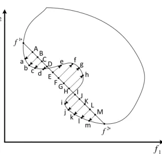
Das and Denis [39] proposed the normal boundary intersection (NBI) method, which at-tempts to find multiple Pareto optimal solutions of a given multiobjective problem by converting it into a number of single objective constrained problems. In the NBI method, it is assumed that the vector of global minima of the objectives (f∗) is available. The convex hull is obtained using the individual minimum of the functions. Then, the simplex is constructed by the convex hull of the individual minimum and is expressed as Φβ. The NBI scalarization scheme takes a point on the simplex and then searches for the maximum distance along the normal pointing toward the origin. This obtained point may or may
0 f1 2 f A a B b C c d ED e F f G g H h I i JKL M j k l m 1 f 2 f
Figure 3.4: Representation of the normal boundary intersection method.
not be a Pareto optimal point. The NBI subproblem for a given vector β is of the form:
maximize : t subject to Φβ+tnˆ =f(x) g(x)≤0 h(x) = 0 x∈Ω (3.2.5) where ∀i ∈ {1, . . . , m} :βi ≥0∧ m P i=1 βi = 1, Φ= [f(x1∗),f(x2∗), . . . ,f(xm∗)] is a m×m
matrix,xi∗ is the minimizer of thei-th individual objective function (xi∗ = arg min
x fi(x)),
ˆ
n is the normal direction at the point Φβ pointing towards the origin. The solution of the above problem gives the maximumt and also the corresponding approximation to the Pareto optimal solution x. The method works even when the normal direction is not an exact one, but a quasi-normal direction. The following quasi-normal direction vector is suggested in Das and Denis [39]: nˆ = −Φe, where e = (1,1, . . . ,1)T is a m×1 vector.
The above quasi-normal direction has the property that NBIβ is independent of the relative
scales of the objective functions.
Figure 3.4 illustrates the working principle of the NBI method. It shows the solutions
0 1 f f2 3 f ) (x3* f Inaccessible regions ) (x1* f f (x2*)
Figure 3.5: Pareto optimal solutions not obtainable using the NBI method.
on the convex hull (Φ= [f1∗ f2∗]) by solving the NBI subproblems for the different vectors β. The method can find solutions in convex and nonconvex regions of the Pareto front. It can be seen that points {f, g, h} are not Pareto optimal but are still found using the NBI method.
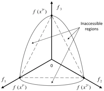
Besides sometimes non-Pareto optimal solutions are obtained, another limitation of the NBI method is that for dimensions more than two, the extreme Pareto optimal solutions are not obtainable in all the cases. This limitation is due to the restriction of 0≤ β ≤1 parameters. This can be easily seen by considering a problem having a spherical Pareto front satisfying f2
1 +f22 +f32 in the range ∀i ∈ {1, . . . , m}: 0 ≤ fi ≤ 1. As seen from
Figure 3.5, there are unexplored regions outside the simplex obtained by the convex hull of individual function minima.
3.2.5
Normal Constraint Method
Messac and Mattson [130] proposed the normal constraint (NC) method for generating a set of evenly spaced Pareto optimal solutions. To describe the NC method, the fol-lowing notations are introduced first. The NC method uses the normalized function values to cope with disparate function scales. The normalized objective vectors (f =
(f1, . . . , fm)T) are computed using the ideal (fideal = (fideal
1 , . . . , fmideal)T) and the nadir
(fnadir = (f1nadir, . . . , fmnadir)T) objective vectors. The following equation is used to perform the mapping: fi = fi−f ideal i fnadir i −fiideal , ∀i∈ {1, . . . , m}.
The points µi∗ = f(xi∗) ∀i ∈ {1, . . . , m} are called the anchor points, where xi∗ is
the minimizer of the i-th objective. The normalized anchor points are denoted as µi∗
∀i ∈ {1, . . . , m}. The m-dimensional hyperplane passing through the anchor points is constructed. A set of evenly distributed point is generated on the hyperplane. Any point on the hyperplane can be defined as a function of the anchor points:
z=Φβ
where z is a point on the hyperplane corresponding to a given vector β which satisfies
∀i∈ {1, . . . , m}: 0≤βi ≤1∧ m X i=1 βi = 1, and Φ= (µ1∗, . . . ,µm∗] is a m×m matrix.
The vectors to fixed anchor point µl∗ from other anchor points are computed:
vi =µl∗−µi∗, ∀i∈ {1, . . . , m} ∧i6=l.
Finally, the NC subproblem for a given point z on the constructed hyperplane is of the form: minimize fl(x) subject to vTi (f(x)−z)≤0, ∀i∈ {1, . . . , m} ∧i6=l g(x)≤0 h(x) =0 x∈Ω (3.2.6)
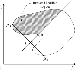
The normal constraint method uses an inequality constraint reduction of the feasible space. Figure 3.6 shows the obtained solution using the NC method for two objectives. The hatched part is the feasible region corresponding to point B in the ideal plane. It can
0 f1
2
f Reduced Feasible Region
1 2
B bFigure 3.6: Representation of the NC method.
be seen that point bis not Pareto optimal but it is still found using the NC method. Since evenly distributed points on the ideal plane are used, the final points on the Pareto front are likely to be more evenly distributed than using the usual -constraint method.
3.2.6
Timmel’s Method
Timmel [174] proposed a stochastic approach for finding multiple Pareto optimal solutions of a differentiable multiobjective optimization problem. It is a population based approach, where for a given parent solution, a child solution is created in the following manner:
xchild =xparent−tk m
X
i=1
ui∇fi(xparent) (3.2.7)
where xparent is the parent decision vector, xchild is the generated child decision vector,
∇fi(xparent) is the gradient of the i-th objective function, tk is the step size at the k-th
iteration and ui is a uniformly distributed random number between zero and one
(ui ∼U(0,1)).
The above formulation ensures that not all objective functions can be worsened simul-taneously. Thus, the child solution xchild is either nondominated when compared to the
0 f1 2 f A B C D a b c d
Figure 3.7: Representation of Timmel’s method.