RESEARCH ARTICLE
Interactive Multi-Objective Particle Swarm Optimisation
with Heatmap Visualisation based User Interface
Jan Hettenhausena†, Andrew Lewisa‡ and Sanaz Mostaghimb§
aInstitute for Integrated and Intelligent Systems, Griffith University, Brisbane, Australia;bAIFB Institute
University of Karlsruhe, Karlsruhe, Germany
(Received 00 Month 200x; final version received 00 Month 200x) This paper introduces an interactive optimisation method based on Multi-Objective Particle Swarm Optimisation that allows a human decision maker to efficiently guide the optimisation process based on his domain specific knowl-edge and experience as well as his problem specific preferences. The method thereby allows inclusion of properties of solutions in the optimisation process which normally would be intractable by computational models. In addition to a modified Multi-Objective Particle Swarm Optimisation algorithm this paper presents a novel graphical user interface based on Heatmap Visualisation which, in combination with the algorithm greatly reduces the workload on a human decision maker, reducing unwanted side effects caused by human fatigue.
The method was evaluated on a set of standard test problems and the results were compared to those of a non-interactive Multi-Objective Particle Swarm Optimisation algorithm. As a common technique to simulate specific prefer-ences and domain specific knowledge of the human decision maker, the decision maker was instructed to focus his search on a previously randomly chosen re-gion of the Pareto front. A qualitative analysis of the results acquired by both methods demonstrates that the introduced method was able to obtain a better solution set than non-interactive Multi-Objective Particle Swarm Optimisation in terms of convergence towards the true global Pareto front and the number of solutions as well as their spread.
Keywords:Interactive Multi-Objective Particle Swarm Optimisation, Heatmap Visualisation, Multi-Objective Optimisation, Interactive Optimisation, MOO Performance Metrics
†Email: [email protected] ‡Email: [email protected]
§Email: [email protected]
ISSN: 0305-215X print/ISSN 1029-0273 online c
200x Taylor & Francis
DOI: 10.1080/0305215YYxxxxxxx http://www.informaworld.com
1. Introduction
The development of sophisticated computational models for many science and engineer-ing applications, in combination with the availability of fast off-the-shelf computengineer-ing sys-tems, makes it possible to employ computational optimisation techniques in various de-sign, development and analysis processes in science and engineering.
Currently the most commonly used techniques are population based, biologically in-spired algorithms which derive their popularity from their comparatively good perfor-mance and their ability to adapt to a wide variety of optimisation problems without requiring exhaustive a priori knowledge. In addition, these methods usually provide good scalability for parallel and distributed computation due to their population based approach.
A relatively new group of methods within this class is Particle Swarm Optimisation and its various derivatives. Particle Swarm Optimisation (PSO) was originally developed by Kennedy and Eberhart in 1995, who derived the biological inspiration from behavioural models of swarming animals such as bird flocks and fish schools (Kennedy and Eberhart 1995, Shi and Eberhart 1998). In PSO this behaviour is modelled by a set of individual particles swarming in the parameter space of the optimisation problem and for each par-ticle an objective function value is calculated. Each of the parpar-ticles maintains a memory of the best solution it has found so far and the swarm maintains a similar memory for either the entire swarm (gbest PSO) or a set of local neighbourhoods of particles within the swarm (lbest PSO). These memories are commonly denoted as the cognitive and so-cial components respectively. Based on these components, in combination with an inertia given by the weighted previous velocity of the particle, a new velocity vector for each particle is calculated in each iteration and used to determine its next position in the parameter space.
Based on single-objective PSO a variety of algorithms have been developed to adapt PSO to optimisation problems with several objectives. These algorithms are commonly referred to as Multi-Objective Particle Swarm Optimisation algorithms (MOPSO). Some of the most common MOPSO variations are presented in Fieldsend and Singh (2002), Moore and Chapman (1999) and Coello and Lechuga (2002).
In multi-objective optimisation the goal is to find an optimal trade-off between several competing objectives for which usually no single optimal solution exists that minimises all objective function values at the same time. Such an optimisation problem can be formally defined as
minimisef(~x) ={f1(~x), f2(~x), ..., fm(~x)} fk:Rn→R,∀~x∈ F,F ⊆ S
(1)
whereF is the feasible space within the search spaceSbased on a set of given constraints. To determine whether one solution is better than another, multi-objective optimisation techniques commonly use the concept of Pareto dominance. A parameter vector x~1 is said to dominate another parameter vectorx~2 if and only if
fk(x~1)≤fk(x~2),∀k∈1, ..., nk
∃k∈1, ..., nk:fk(x~1)< fk(x~2)
All non-dominated solutions form the Pareto-optimal set in parameter space
P∗ ={x~∗∈ F |
@~x∈ F :~x≺x~∗} (3) The set of vectors in objective space corresponding to the parameter vectors of the Pareto optimal set are denoted as the Pareto front.
PF∗={f(x~∗)|x~∗ ∈ P} (4)
For two different solutions from the Pareto-front there exists, however, no generally ap-plicable definition to further distinguish their quality. Doing so requires a human decision maker to select those solutions he considers best for the desired purpose. Van Veldhuizen and Lamont (2000) distinguish between three different stages of the optimisation process where this selection can take place.
A priori selection is applied before the optimisation process is started. Usually this is achieved by using a weighting function which provides a mapping of all objectives to a one-dimensional fitness value. While these individual weights are usually well known, on certain types of Pareto-fronts this approach often fails to find all solutions.
A posteriori based approaches employ the optimisation heuristic to discover as many non-dominated solutions as possible. They mainly aim for a wide and even spread of these solutions over the entire Pareto front. After the algorithm has terminated the decision maker is presented with all available solutions and can then select the ones preferred.
The third category is formed by the progressive methods which employ the deci-sion maker to articulate preferences during the optimisation process allowing dynamical change of preferences as new solutions arise. Many methods that fall into this category are of the Interactive Evolutionary Computation paradigm. This paradigm includes all Evolutionary Computation-based methods that involve human interaction of some sort. The progressive methods belong to a subclass of IEC which Takagi (2001) describes as the “broader definition” of Interactive Evolutionary Computation. Takagi considers all methods involving a human-machine interface fall into this broader definition, whereas those methods falling into his narrow definition only include those that employ the de-cision maker as a source of objective function values directly.
Involving a human decision maker during the optimisation process for a multi-objective problem provides several significant advantages. Assuming the human decision maker has some knowledge of the field the optimisation problem belongs to, he can evaluate trial solutions based on a large set of criteria at the same time and include criteria for which no mathematic formulation exists. Such criteria can on the one hand render solutions unfeasible that otherwise perform well in terms of the mathematically defined objectives, but they can also make solutions more preferable even though their performance might otherwise be slightly inferior to other solutions. For an example of the benefit from this, the reader is referred to Kamalian et al. (2004) where user interaction is applied to a MEMS design problem.
Although the majority of publications focus on IEC in Takagi’s narrow definition, an increasing number of works have been published on progressive optimisation using IEC (Takagi 2001, Kamalianet al. 2004, 2006). In contrast, very few efforts have been made to date to adapt Particle Swarm Optimisation1for user interaction, even though PSO has
1Although many publications regard PSO as part of the EC paradigm, the structural and con-ceptual differences of PSO, which have particular relevance to interactive optimisation, justify its
several interesting properties which can improve user fatigue-related problems common to IEC-based methods. In addition, Yu, Xiong and Wu (Yu et al. 2004) argue that for many test problems PSO shows a better convergence than Genetic Algorithms, which are a major group within Evolutionary Computation, making the extension to interactive methods for PSO even more desirable.
To date, the authors were able to find only two other approaches to Interactive Particle Swarm Optimisation (Agrawalet al.2008, M´aderet al.2005) and one approach that uses a priori articulated user preferences in a PSO algorithm (Wickramasinghe and Li 2008). These approaches will be briefly discussed in Section 2. The small number of approaches can partially be attributed to the fact that PSO is a relatively new optimisation technique but also to the problem of incorporating a decision maker into the social interaction model of PSO which, in contrast to other IEC algorithms, has a memory of previous good solutions.
This paper introduces a new approach to Interactive Multi-Objective Particle Swarm Optimisation which potentially improves human fatigue related problems by means of a new user interaction model in combination with a novel user interface concept, based on Heatmap Visualisation (Prykeet al.2007) and ideas from visual analytics (Thomas and Cook 2006, Cardet al.1999). With a MOPSO algorithm as its basis the method described also employs Pareto dominance as a measure of solution quality whereas the majority of progressive optimisation methods use aggregation based approaches in combination with single-objective optimisation methods. This allows the human decision maker to effectively guide the swarm with minimal effort.
The following section will describe the modified MOSPO algorithm as well as the graphical user interface. The remainder of the paper will provide an evaluation of the method in comparison to a standard MOPSO algorithm.
2. Interactive Multi-Objective Particle Swarm Optimisation
Interactive Multi-Objective Particle Swarm Optimisation (IMOPSO) aims to combine the capabilities and advantages of Multi-Objective Particle Swarm Optimisation with the domain specific knowledge and experience of a human decision maker. This allows optimisation of problems based on mathematically formulated objectives as well as guid-ing optimisation based on objectives for which no computational model exists but which may be simple for a human decision maker to evaluate.
2.1. Related Work
The number of user preference based Particle Swarm Optimisation methods is still rea-sonable small and most methods today rely ona posteriori selection of results. Among the user preference based methods, Wickramasinghe and Li (2008) introduced a MOPSO algorithm that is based ona prioriselected reference points in objective space. The prox-imity of globally non-dominated solutions to these reference points then influences their ability to be selected as global guide solutions during the optimisation process.
A first progressiveapproach to Particle Swarm Optimisation was developed by M´ader et al. (2005) who used a single objective PSO in which the user selects the global and
classification as a Computational Swarm Intelligence optimisation method distinct from EC. For a detailed discussion on this matter the reader is referred to Engelbrecht (2005, p. 126).
local guides. The approach can be considered as an aggregated approach with an im-plicit aggregation function presented through the user selections. Their IPSO algorithm, however, requires the user to evaluate every single solution which effectively reduces the possible number of particles and iterations severely in order to avoid loss of quality due to human fatigue.
Anotherprogressiveapproach aiming at developing an interactive Multi-Objective Par-ticle Swarm Optimisation was made by Agrawalet al. (2008). In essence, this approach attempts to reduce the workload on the decision maker by querying the decision maker only after a finitely large archive of non-dominated solutions reaches a set capacity limit. The decision maker is then presented with known non-dominated solutions which are further filtered using a weighting function that is constructed of previously made selec-tions. The role of the human decision maker is then to select preferable solutions from this filtered set of non-dominated solutions by means of pair-wise comparison. The ap-proach also incorporates adaptive grid principles to bias the algorithm’s selection of guide particles in each iteration.
The method presented in this paper is distinctively different in several key aspects to the aforementioned methods. The most significant of these is the way the interaction with the human decision maker is carried out. To allow a more effective user interaction with less restrictions in terms of swarm size and user fatigue, the proposed IMOPSO method employs a novel user interface design to limit the workload on the decision maker by presenting the data in a way more suitable for the human brain to process. This user interface, in contrast to the user interfaces used for the methods of Agravalet al.and M´aderet al., imposes only a minimum of restrictions on the number of solutions presented to the decision maker and the size of the swarm without aggravating human fatigue. While the method of Agraval et al. does not restrict the size of the swarm, it severely limits the number of solutions the decision maker may choose from. Based on the work by Kamalianet al.(2004) this appears to be undesirable as a human decision maker might apply criteria to evaluate the quality of a solution which may not be tractable by the applied mathematical critera, i.e. the objective functions. Such criteria might, for example, make a dominated solution preferable over a non-dominated solution.
Apart from the different ways user interaction is implemented, the aim of the IPSO approach of Agraval et al.was to achieve a more even distribution of solutions over the entire Pareto whereas the method presented in this paper is an attempt provide a high level of influence to the human decision maker, allowing the search to be focussed on any interesting region of the Pareto-front and obtain faster convergence and improved spread and solution density in this region.
2.2. IMOPSO Algorithm
The Interactive Multi-Objective Particle Swarm Optimisation algorithm presented in this paper is based on a standardgbestMOPSO algorithm and incorporates user interaction via the velocity vector update equation. The choice of agbestapproach was made since it allows the swarm to rapidly react to changes in the decision maker’s preferences and is generally faster to converge thanlbest MOPSO approaches (Engelbrecht 2005).
In non-interactive MOPSO the velocity update is based on the following equation: ~vg+1 =wg·~vg+c1r1(ˆypbest−xg) +c2r2(ˆygbest−xg) (5) The new velocity is therefore based on the statically weighted previous velocity andpbest
andgbestguide solutions which are each weighted with a constant factor and a random value. Commonly the constant factors are chosen to be 2 and the random factor to be evenly distributed between 0 and 1. This causes the overall factor to either over- or undershoot the guide with the same probability. A variety of different strategies exist to select a guide from the archive, among which random selection still remains the most generally applicable without imposing problem specific preferences (Irelandet al. 2006, Mostaghim and Teich 2003, Coello and Lechuga 2002, Fieldsend and Singh 2002).
Based on the previous position in parameter space and the new velocity a new position is calculated in each iteration as
xg+1 =xg+vg (6)
To add user interaction to MOPSO the proposed method replaces the social component of the swarm with a new component which, rather than being chosen from an archive of previously-found good solutions, is chosen from a set of solutions that a human decision maker has selected. Each particle in the swarm randomly chooses itsgbest guide from this set instead of from thegbestarchive. This set of selected solutions is denoted as the gbestselected. The gbestarchive of non-dominated solutions is, however, still maintained to supply information on globally non-dominated solutions to the decision maker but it no longer influences the velocity update. The velocity update equation in IMOPSO therefore takes the following form (the indices of the coefficients of the new component are incremented to 3 to make the change apparent)
~vg+1 =wg·~vg+c1r1(ˆypbest−xg) +c3r3(ˆygbestselected−xg) (7) The pbestcomponent in IMOPSO was left unchanged to limit the input required from the human decision maker. However, in contrast to most MOPSO approaches, it is based on an archive of non-dominated solutions for each particle rather than a single solution memory. Furthermore the pbest guide for each particle in each iteration is selected to be the solution with the closest Nearest-Neighbour Method proximity to any one of the solutions in the gbestselected group, based on Euclidian distance. Formally expressed the selection is based on the following equation:
ˆ
ypbest ={y|mind(x, y), x∈ygbestselected, y ∈ypbest} (8) Performing the guide particle selection like this ensures fast convergence to the area of the parameter space which the decision maker is interested in without requiring him to provide any further guidance than choosing the gbestselected solutions. An unwanted side effect of this is, however, that in some cases where the decision maker selects only a very small number of solutions in an early stage of the optimisation, all particles assume a similar value for a parameter and the swarm ceases to move in that dimension of parameter space. To compensate such “clinging” behaviour, a “craziness” component (Kennedy and Eberhart 1995), which adds a random turbulence to the velocities, was added to the position update equation:
xg+1=xg+vg+χ~ (9)
intensity of the turbulence on the relative movement of each particle in each dimension of parameter space. Essentially such turbulence only occurs when the velocity of the particle in a particular parameter n slows down to a value that causes less than 8% change in relation to the feasible range of this parameter. The following equation formally defines this turbulence: χn= 0 vgn≥0.03(xnmax−xnmin) fX(0, σn) else (10)
The intensity of the turbulence is given by fX(0, σ), a Gaussian distributed random variable with an average of zero and a standard deviation
σn= 0.08− v n g xn max−xnmin (11) which decreases the probability of a high turbulence with increasing velocity.
The reader is directed to Algorithm 1 for a pseudocode implementation of the proposed method.
Algorithm 1Interactive MOPSO Initialise iterationi= 0;
Initialise swarmS withnparticles; Evaluate S;
foreach particlep inS do Initialise velocity~v=~0; Initialise p.pbest; end for
Initialise gbestarchive; repeat
Query decision maker forgbestselectedi; foreach particlep inS do
Randomly select ˆygbestselected fromgbestselectedi; Select ˆypbest using equation (8)
Update velocity using equation (7); Update position using equation (9); end for
Evaluate S;
foreach particlep inS do Updatep.pbest; end for
Updategbestarchive; i=i+ 1;
until i==imax or decision maker stops manually
The structure of the IMOPSO algorithm allows guiding the optimisation by only se-lecting some non-zero number of solutions which the decision maker considers best, based on professional experience, domain knowledge and problem specific preferences. It also eliminates the need for the decision maker to review every solution in detail which po-tentially reduces the workload significantly. While the algorithm provides an effective
basis for this, the actual workload reduction is achieved by the user interface. The next section will discuss a novel approach to user interaction which was designed specifically for this purpose.
2.3. User Interface
The user interface is a crucial component of any interactive optimisation technique. A good user interface can support the user in making good decisions and reaching these decisions in a short time. The majority of user interfaces in Interactive Evolutionary Computation present all results to the user, usually in the form of a plot or graphical representation of each individual design (Kamalianet al.2004, 2006, M´ader et al.2005) or by a tabular representation of the data (Todd and Sen 1999). The majority of previ-ous approaches requires the user to review every individual solution to make a selection or come to a rating. The design goal for the user interface in IMOPSO was to avoid the need for the user to review all solutions to come to a decision. With only a small number of guide particles necessary for the IMOPSO algorithm the user should be able to focus on the solutions of interest within a very short amount of time and only review those particular solutions more closely. A solution to this is provided by the concept of Visualised IEC (Hayashida and Takagi 2000, Takagi 2000) which uses graphical rep-resentations of solution spaces to supply the user with additional information. Typical visualisation methods for this are 2D and 3D space plots and self-organised maps. Space plots, however, are limited to problems with two or three objectives only and cannot represent the parameters and objectives for each candidate solution in the same plot. Self-Organised Maps do not suffer from this limitation but, as with space plots, are usu-ally restricted to visualising either the objective space or the parameter space thereby losing the visual correlation of the two as a supplemental source of information.
To make as much information as possible easily accessible raised the need for another visualisation method which overcomes the shortcomings of the aforementioned methods. To be effective it had to incorporate basic principles of visual analytics (Thomas and Cook 2006, Cardet al. 1999) and allow extension to an interactive visualisation method also based on visual analytics principles. A major reason for continuously assessing the GUI design against these principles is to allow objective evaluation of its quality. Furthermore, a mainly visual interface is capable of reducing the workload on the decision maker by providing the information in a form that is most suitable for a human user. Human information processing is, to a large extend, a visual process and the human brain can easily process large amounts of visual data and recognise patterns and structures that would likely be less apparent if presented non-graphically. Cardet al. (1999) summarise the main points of how data visualisation can be designed in order to support these capabilities:
• Increased resources: visualisation allows for humans to process information in parallel which is usually not possible for data in textual form. In addition, visually presented information increases the available working memory and allows presentation of large amounts of information that is easily accessible when used appropriately.
• Reduced search: the high information density possible in visual representations reduces the need for searching within the data.
• Enhanced Recognition of Patterns:organising data by structural relationships enhances the recognition of patterns
• Perceptual Inference: visualised data can support reasoning on data relationships and patterns which in other forms of presentation may not be apparent.
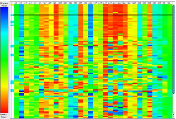
Figure 1. User Interface based on Heatmap Visualisation.
• Perceptual Monitoring: visualisation can allow monitoring of a large number of poten-tial events.
• Manipulable Medium: a manipulable presentation allows the user to explore the data in the given space.
The user interface proposed in this paper will use a modified Visualised IEC approach for the user interaction to accommodate the benefits of the underlying IMOPSO algo-rithms. Rather than using the visualisation of the result space as supplementary infor-mation to the user, it will be used as the primary means of data representation. This allows a decision maker to rapidly identify those solutions which have interesting proper-ties and ignore all other solutions. Presenting the information graphically also allows the size of the swarm to be increased significantly in comparison to the IPSO approach by M´aderet al., as the review of all solutions is reduced to identifying interesting patterns and a close up review is only required for the (usually) small set of interesting solutions. Limitations on the swarm size caused by the interaction are therefore mainly limited to the capabilities of the visualisation method.
Among the visualisation methods that allow visualisation of higher dimensional spaces the Heatmap Visualisation by Pryke et al. (2007) seemed to provide an ideal basis for the user interface as it has virtually no limitations on the size of the visualised space. In addition, it is the only visualisation method that incorporates a structural correla-tion between input parameters and their corresponding objective funccorrela-tion values. These properties particularly support the concepts of perceptual inference and enhanced recog-nition. Self-organised Maps, though also a highly interesting visualisation method, did not provide the same flexibility as Heatmap Visualisation and also do not incorporate
the input parameters in the same plot. Approaches that use two self-organised maps and include plots of solutions in these (Obayashi and Sasaki 2003) partially solve this problem but contradict the idea of keeping the user interface simple and straightforward. In the standard view of Heatmap Visualisation the data is organised in rows and columns, each row representing a candidate solution and each column either a parameter or an objective to the optimisation problem. To support the perception of visual patterns the data, by default, is hierarchically clustered based on the Euclidian distance in param-eter space of the solutions to each other. For the user interface the Heatmap Visualisation was extended with sorting capabilities so a user can sort the data by any of the columns or several columns hierarchically. The columns were also designed to be interchangeable, allowing the user to manually organise and group parameters and objectives. With these enhancements the user interface becomes a manipulable medium which allows the user to interactively explore the available solutions.
A key issue of integration of the user interface and the IMOPSO algorithm is what type of solutions the user should be able to select from. It is safe to assume that in a multi-objective optimisation problem the non-dominated solutions are more interesting to a user than other solutions unless solutions are interesting for other reasons, such as their their parameter values or non-computationally tractable properties. The user interface therefore presents solutions from the archive of globally non-dominated solutions, the solutions selected in the previous iteration and all particles of the swarm at their current positions. Assuming that a decision maker will select interesting solutions this subset of all known candidate solutions effectively limits the number of solutions to a feasible amount without discarding any relevant solutions. An additional column was introduced in the Heatmap view that graphically indicates whether a solution is non-dominated, previously selected, both or neither.
To accommodate problem or user-specific needs the Heatmap Colour Scale can be changed to a Grayscale Colour Scale and a Red and Blue Colour Scale. In addition, the mapping to the selected colour scale can be changed from linear to logarithmic for each column individually to provide easier handling for columns with solutions spanning orders of magnitudes.
An example of the Heatmap Visualisation based user interface can be seen in Figure 1. The example uses the standard colour scale. Rows marked blue in the first column are non-dominated solutions. For previously selected solutions this field would be yellow or yellow and blue for solutions falling into both categories.
In addition to the graphical view the user interface also provides the underlying data in a table and a plot of the design for each solution should there be one available. Both these alternative representations of the data are automatically represented to the user when a solution is selected. However, the Heatmap View always remains on the screen as well, allowing location of the current solution in the space of available solutions. Ideally the decision maker will only review this additional data for a few solutions that appear particularly interesting.
As the GUI design makes use of modified Heatmap Visualisation to present the data to the user, it inherits some of its properties regarding user perception of the data. In the terminology of visual analytics these are explicitlyincreased resources andreduced search, mainly for the reason that large amounts of data can be presented in a way that is easy to view, parse and search. In fact, the possibility to conveniently visualise large amounts of data without overwhelming the user with information but also without omitting relevant parts of the data make it a quite popular graph type in many applications that involve excessive amounts of data, such as the DNA microarray analysis in biology. As one of the
primary causes of human fatigue is dealing with an overwhelming amount of information, the usage of Heatmap Visualisation provides a possible means of reducing human fatigue by presenting the information in a more appropriate way.
In additon, enhanced recognition of patterns and perceptual inference are implicitly supported by the GUI as a secondary result of the presentation in a Heatmap chart. Heatmaps as a chart type make the recognition of patterns particularly easy as the data is organised in rows and columns for the candidate solutions and the parameters and objectives. Solutions and properties can therefore be arranged and sorted to make their similarities and differences visually apparent. Also, the mapping of numerical data to a temperature-like scale enhances intuitive recognition of patterns.
In contrast to other types of visualisation, reasoning and pattern recognition is therefore not limited to either the parameter or objective space. Instead, the interface allows effective review of the complete set of candidate solutions at the same time without overwhelming the user with the amount of information. This particular property is one of the main arguments that distinguished the proposed Heatmap Visualisation-based GUI from other user interfaces for interactive optimisation. Another is that despite viewing large numbers of candidate solutions, the user can still clearly identify and select each individual solution in a very simple and straightforward fashion.
By employing Heatmap Visualisation the proposed user interface therefore implic-itly makes use of a variety of concepts of visual information processing. The proposed additions to Heatmap Visualisation to turn it into a User Interface for Interactive Opti-misation implement two additional visual analytics principles, as they make the medium manipulable in each iteration, allowing active exploration and reasoning on the data, and to some extent it also facilitatesperceptual monitoring, as over the course of several iterations the user is provided with the ability to keep track of and analyse changes in a number of areas of the candidate solution space.
3. Evaluation
The proposed method will be evaluated on a set of well known test problems. The design of the tests is slightly different to other tests for multi-objective optimisation methods since its main focus is to test the difference between the proposed interactive MOPSO approach and a non-interactive MOPSO in a region of the decision makers interest. To do so, the human decision maker was instructed to guide the search to a particular region of the Pareto front which simulates a preference he would have in a real-life optimisation problem. The region was essentially randomly chosen from the known Pareto front except that extremal areas of the objective space were intentionally excluded to avoid possible algorithm-specific biases. In the following, the selected region will be denoted as the “focus region”. This test approach for an interactive optimisation method is based on a similar test design previously used by Todd and Sen (1999).
3.1. Test Cases
To demonstrate the capabilities of Interactive Multi-Objective Particle Swarm Optimi-sation three common test functions, each featuring typical challenges to multi-objective optimisation algorithms, were chosen. The test functions were taken from Zitzler (1999) and follow the same general structure:
minimiset(x) =(f1(x1), f2(~x))
subject to f2(~x) =g(x2, ..., xn)·h(f1(x1), g(x2, ..., xn)) where~x=(x1, ..., xn)
(12)
3.1.0.1. Test function 1. The test function, denoted by Zitzler as t1, has a convex Pareto front: f1(x1) =x1 g(x2, ..., gn) = 1 + 9· Pn i=2xi n−1 h(f1, g) = 1− s f1 g (13)
withn= 30 and x1 ∈[0,1]. The global Pareto front is formed withg= 1.
3.1.0.2. Test function 2. The test function, denoted by Zitzler as t2, has a non-convex Pareto front: f1(x1) =x1 g(x2, ..., gn) = 1 + 9· Pn i=2xi n−1 h(f1, g) = 1− f1 g 2 (14)
withn= 30 and x1 ∈[0,1]. The global Pareto front is formed withg= 1.
3.1.0.3. Test function 3. The test function, denoted by Zitzler ast3, has a discontinuous Pareto front consisting of several convex parts:
f1(x1) =x1 g(x2, ..., gn) = 1 + 9· Pn i=2xi n−1 h(f1, g) = 1− s f1 g −f1 g sin 10πf1 (15)
withn= 30 and x1 ∈[0,1]. The global Pareto front is formed withg= 1. The disconti-nuity of the Pareto front does not extend to the objective space itself and is caused by the sine function inh(f1, g).
Table 1. Parameter Settings for IMOPSO and MOPSO as used for the test cases.
Method w c1 c2 c3 swarm size
MOPSO 0.4 2.0 2.0 0.0 100 IMOPSO 0.4 2.0 0.0 2.0 100
to evaluate a multi-objective optimisation method and results from such tests are also valid for higher dimensional problems.
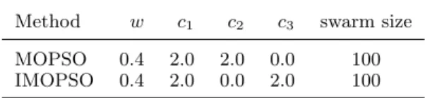
The number of iterations used for the tests was relatively low, given that most algorithm used on Zitzler (1999) needed 250 or more iterations to find solutions on the actual Pareto front. This was done for two reasons. Firstly, it allows a qualitative comparison of the interactive and non-interactive MOSPO algorithm by giving a clear indication of the speed with which each algorithm converges towards the Pareto front, or some selected region of it, and it also provides for an analysis of the number of solutions found in a particular area. Secondly, the quality of interactive optimisation methods is influenced by human fatigue when the number of ratings or selections that the user has to make becomes excessively large. A relatively small number of such ratings, however, can be considered free of such an influence and therefore provides a fairer comparison of algorithmic capabilities. Future research will focus on improvements to compensate for human fatigue-related problems and allow increasing numbers of iterations. Based on the fact that both methods are “anytime” algorithms, that is, they can be stopped at any time and return the best known solution at the time of interruption, it is safe to assume that limiting the number of iterations has no influence on the validity of the test results. The majority of tests was therefore conducted with 25 iterations. However, to illustrate that the IMOPSO retains its capabilities at higher iterations as well, an additional run with 100 iterations was performed for each of the test functions. Table 1 provides a summary of the parameters used for the tests.
3.2. Performance Measures
Multi-objective optimisation problems are usually compared based on their convergence towards the Pareto-optimal set and the diversity and spread over the Pareto front that the obtained solutions provide. Debet al.(2002) argue that no single metric can be used to assess both these qualities at the same time and therefore two metrics are necessary to evaluate the result set of an algorithm. One of these is employed to evaluate the distance to the actual Pareto-front, the second one to measure the coverage of the approximated front in comparison to the full extent of the actual Pareto-front.
As the actual Pareto fronts were known for all three test functions, the Υ metric of Deb et al.(2002) was used to measure the convergence towards the Pareto-front. To calculate the score for this metric, a large but finite set of equal spaced points covering the actual Pareto-front has to be known. For each of the solutions in the set of solutions obtained by the algorithm evaluated, the Euclidian distance to the nearest point of a set of points sampled from the true Pareto-front is calculated. The average of all these distances is defined as the Υ score for the approximated Pareto-front.
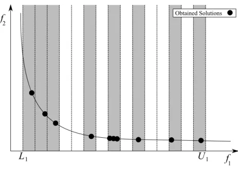
To evaluate the coverage of each method a new performance measure Ψ is introduced here. For a two-dimensional problem, one of the objectives is selected and the respective
Figure 2. Diversity metric Ψ
dimension of the objective space is split into a number of equally sized intervals ψn, where the number of intervals is defined as the maximum of the size of the swarm and the size of the archive. Each of these intervals is inspected to see if a non-dominated solution lies between the upper and lower bounds of the interval. If at least one such particle exists, the interval is scored 1, otherwise its score is set to 0. The metric is given by the percentage of of “occupied” intervals. It is thus a measure of the total extent of the Pareto-front covered, and the uniformity of the coverage. Figure 2 illustrates this metric. The calculation can be formalised as
Ψ = 100 max{|A|,|S|} max{|A|,|S|} X n=1 ψn (16)
whereA and S represent the size of the archive and the size of the swarm respectively. The individual “buckets”ψn are then defined as
ψn
(
1, if∃f(~~ x)∈ PF, βn−1≤f1(~x)< βn
0, else (17)
with f1 being one of the objectives and βn defining the upper boundary for bucket n. Any objective can be chosen to bef1 but the same objective has to be used for all the buckets for obvious reasons. The upper boundaries for the bucketsβnare defined as
βn=L1+n·
U1−L1
max{|A|,|S|} (18)
where U and L mark the upper and lower boundaries of the analysed portion of the Pareto-front based on the chosen objectivef1. The lower boundary for bucketnis defined
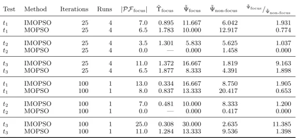
Table 2. Comparison of Interactive- and Non-Interactive Multi-Objective Particle Swarm Optimisa-tion.
Test Method Iterations Runs |PFfocus| Υ˜focus Ψ˜focus Ψ˜non-focus ˜ Ψfocus/ ˜ Ψnon-focus t1 IMOPSO 25 4 7.0 0.895 11.667 6.042 1.931 t1 MOPSO 25 4 6.5 1.783 10.000 12.917 0.774 t2 IMOPSO 25 4 3.5 1.301 5.833 5.625 1.037 t2 MOPSO 25 4 0.0 — 0.000 1.458 0.000 t3 IMOPSO 25 4 11.0 1.372 16.667 1.819 9.163 t3 MOPSO 25 4 6.5 1.877 8.333 4.391 1.898 t1 IMOPSO 100 1 13.0 0.334 16.667 8.750 1.905 t1 MOPSO 100 1 8.0 0.837 13.333 20.417 0.653 t2 IMOPSO 100 1 7.0 0.481 10.000 8.333 1.200 t2 MOPSO 100 1 0.0 — 0.000 0.417 0.000 t3 IMOPSO 100 1 25.0 0.308 30.000 2.635 11.385 t3 MOPSO 100 1 11.0 1.284 13.333 9.536 1.398
asβn−1. Higher order problems can be scored by extending the bucket definition to the respective number of dimensions.
To demonstrate the abilities of the Interactive MOPSO to focus the search on a par-ticular area of the Pareto-front, the Ψ was calculated for the focus and non-focus regions of the Pareto front and used to calculate a ratio between the coverage within and outside the focus region. The bucket size for the non-focus area was chosen to be identical to the bucket size inside the focus region.
3.3. Discussion of the Results
The goal for the proposed Interactive Multi-Objective Particle Swarm Optimisation was to focus the optimisation process on a particular region of the Pareto-front, the focus region, and achieve a better convergence and greater coverage of the approximate Pareto-front within this region. The focus region thereby simulates a decision maker’s preferences as they would appear in a real-life optimisation problem and was chosen to be between values of 0.5 and 0.7 for the first objective for all three test problems. Table 2 summarises the results of the tests performed.
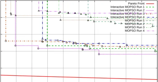
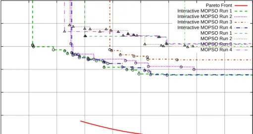
The results for IMOPSO on test functiont1 andt3 consistently show a greater conver-gence towards the actual Pareto-front after 25 iterations as well as after 100 iterations. The coverage within the focus region is also higher than for the standard MOPSO. The Ψ values fort1 are only slightly better after 25 iterations but increase significantly with further progress. The Ψfocus/Ψnon-focus ratio for all results shows that the Interactive MOPSO could be effectively concentrated on the focus region for both functions. Fig-ures 3and 5 provide illustration of the approximate Pareto-fronts acquired by Interactive-and non-interactive MOPSO on test functiont1 and t3.
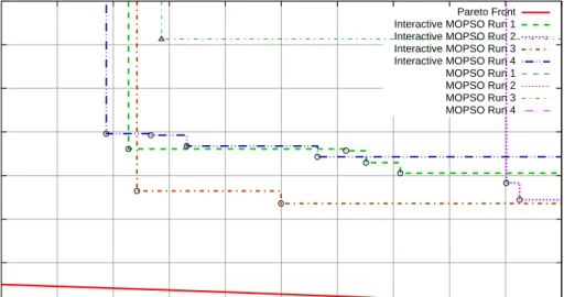
The second test function (t2) is an exceptional case as the standard MOPSO was un-able to find any non-dominated solutions in the focus region in the majority of runs. This is a well-known but often unacknowleged problem of common non-interactive MOPSO implementations. While the lack of results from non-interactive MOPSO in the focus
0 0.5 1 1.5 2 2.5 0.5 0.52 0.54 0.56 0.58 0.6 0.62 0.64 0.66 0.68 0.7 Objective 2 Objective 1 Test function t1 (25 iterations)
Pareto Front Interactive MOPSO Run 1 Interactive MOPSO Run 2 Interactive MOPSO Run 3 Interactive MOPSO Run 4 MOPSO Run 1 MOPSO Run 2 MOPSO Run 3 MOPSO Run 4 0 0.2 0.4 0.6 0.8 1 1.2 1.4 0.5 0.52 0.54 0.56 0.58 0.6 0.62 0.64 0.66 0.68 0.7 Objective 2 Objective 1 Test function t1 (100 iterations)
Pareto Front Interactive MOPSO MOPSO
Figure 3. Comparison of the achieved attainment surfaces in the focus area for Interactive Multi-Objective Particle Swarm Optimisation and non-interactive Multi-Multi-Objective Particle Swarm Op-timisation on Zitzlers test functiont1 as described in equation (13).
region of t2 makes a qualitative comparison impossible, it clearly shows that the pro-posed interactive MOPSO can be guided into regions of the objective space which are otherwise inaccessible and provide good convergence and coverage within these as Figure 4 illustrates.
In summary, Interactive MOPSO could provide better results within the focus region compared with a non-interactive MOPSO in all three test cases. The tests also show that it is easy to guide the swarm to the region of interest with reasonably low effort on the
0.5 1 1.5 2 2.5 3 3.5 4 0.5 0.52 0.54 0.56 0.58 0.6 0.62 0.64 0.66 0.68 0.7 Objective 2 Objective 1 Test function t2 (25 iterations)
Pareto Front Interactive MOPSO Run 1 Interactive MOPSO Run 2 Interactive MOPSO Run 3 Interactive MOPSO Run 4 MOPSO Run 1 MOPSO Run 2 MOPSO Run 3 MOPSO Run 4 0.5 0.6 0.7 0.8 0.9 1 1.1 1.2 1.3 1.4 0.5 0.52 0.54 0.56 0.58 0.6 0.62 0.64 0.66 0.68 0.7 Objective 2 Objective 1 Test function t2 (100 iterations)
Pareto Front Interactive MOPSO MOPSO
Figure 4. Comparison of the achieved attainment surfaces in the focus area for Interactive Multi-Objective Particle Swarm Optimisation and non-interactive Multi-Multi-Objective Particle Swarm Op-timisation on Zitzlers test functiont2 as described in equation (14).
part of the human decision maker.
4. Conclusion
This paper introduced a new method to interactively find solutions for a multi-objective optimisation problem using Multi-Objective Particle Swarm Optimisation as a
founda--0.5 0 0.5 1 1.5 2 2.5 0.59 0.6 0.61 0.62 0.63 0.64 0.65 0.66 0.67 0.68 Objective 2 Objective 1 Test function t3 (25 iterations)
Pareto Front Interactive MOPSO Run 1 Interactive MOPSO Run 2 Interactive MOPSO Run 3 Interactive MOPSO Run 4 MOPSO Run 1 MOPSO Run 2 MOPSO Run 3 MOPSO Run 4 -0.5 0 0.5 1 0.59 0.6 0.61 0.62 0.63 0.64 0.65 0.66 0.67 0.68 Objective 2 Objective 1 Test function t3 (100 iterations)
Pareto Front Interactive MOPSO MOPSO
Figure 5. Comparison of the achieved attainment surfaces in the focus area for Interactive Multi-Objective Particle Swarm Optimisation and non-interactive Multi-Multi-Objective Particle Swarm Op-timisation on Zitzlers test functiont3 as described in equation (15).
tion. The proposed method is a combined approach of a modified MOPSO algorithm and a novel user interface based on Heatmap Visualisation that graphically presents the space of available solutions to a human decision maker. Such a method allows the deci-sion maker to quickly find solutions of interest and guide the algorithm towards these regions. The combination of user interface and algorithm, in contrast to common IEC based approaches, eliminate the need for the decision maker to review or rate all avail-able solutions. Instead only those solutions that appear most feasible from the graphical
overview need to be reviewed.
The method was tested against a standard MOPSO algorithm on three common multi-objective test problems which represent typical challenges as they are encountered in real-life optimisation problems. For each test problem the human decision maker was in-structed to focus the search on a particular region. On all three test functions the decision maker was able to focus the search on a region of interest and gather significantly better results there. Furthermore, the Interactive MOPSO was able to achieve good results in regions within which the non-interactive MOPSO was unable to find any solutions at all. The results indicate that the method can be highly beneficial for problems where the computation of a single solution is expensive or very time consuming so that reducing the overall time by involving a human decision maker reduces the total cost for the optimisation. This is particularly relevant to engineering applications, which often require complex simulations based on FEM or FDM to acquire a single solution. In addition, user interaction appears to be a desirable feature for optimisation problems where non-interactive optimisation techniques fail to find a sufficient number of non-dominated solutions.
Acknowledgements
The authors would like to thank Andy Pryke for his encouragement and assistance with the Heatmap Visualisation method.
References
Agrawal, S., et al., 2008. Interactive Particle Swarm: A Pareto-Adaptive Metaheuris-tic to Multiobjective Optimization. Systems, Man and Cybernetics, Part A, IEEE Transactions on, 38 (2), 258–277.
Card, S.K., Mackinlay, J.D., and Shneiderman, B., 1999. Using vision to think. San Francisco, CA, USA: Morgan Kaufmann Publishers Inc.
Coello, C. and Lechuga, M., 2002. MOPSO: A Proposal for Multiple Objective Particle Swarm Optimization.In:Evolutionary Computation, 2002. CEC’02. Proceedings of the 2002 Congress on, Vol. 2 IEEE Computer Society.
Deb, K., 1999. Multi-objective Genetic Algorithms: Problem Difficulties and Construc-tion of Test Problems.Evolutionary Computation, 7 (3), 205–230.
Deb, K.,et al., 2002. A fast and elitist multiobjective genetic algorithm: NSGA-II. Evo-lutionary Computation, IEEE Transactions on, 6 (2), 182–197.
Engelbrecht, A., 2005.Fundamentals of Computational Swarm Intelligence. John Wiley & Sons, Ltd.
Fieldsend, J. and Singh, S., 2002. A multi-objective algorithm based upon particle swarm optimisation.Proceedings of The UK Workshop on Computational Intelligence, 34– 44.
Hayashida, N. and Takagi, H., 2000. Visualized IEC: Interactive evolutionary computa-tion with multidimensional data visualizacomputa-tion. Industrial Electronics, Control and Instrumentation (IECON2000).
Ireland, D., et al., 2006. Hybrid Particle Guide Selection Methods in Multi-Objective Particle Swarm Optimization.In:E-SCIENCE ’06: Proceedings of the Second IEEE
International Conference on e-Science and Grid ComputingWashington, DC, USA: IEEE Computer Society, p. 116.
Kamalian, R., Takagi, H., and Agogino, A.M., 2004. Optimized Design of MEMS by Evo-lutionary Multi-objective Optimization with Interactive EvoEvo-lutionary Computation. In:GECCO-2004Springer Verlag, 1030–1041.
Kamalian, R.,et al., 2006. Reducing Human Fatigue in Interactive Evolutionary Com-putation through Fuzzy Systems and Machine Learning Systems.In:IEEE Interna-tional Conference on Fuzzy SystemsIEEE Computer Society.
Kennedy, J. and Eberhart, R., 1995. Particle swarm optimization.Neural Networks, 1995. Proceedings., IEEE International Conference on, 4.
M´ader, J., Abonyi, J., and Szeifert, F., 8-10 Sept. 2005. Interactive particle swarm opti-mization.Intelligent Systems Design and Applications, 2005. ISDA ’05. Proceedings. 5th International Conference on, 314–319.
Moore, J. and Chapman, R., Application of Particle Swarm to Multiobjective Opti-mization. , 1999. , Technical report, Department of Computer Science and Software Engineering, Auburn University.
Mostaghim, S. and Teich, J., 2003. Strategies for finding good local guides in multi-objective particle swarm optimizationoptimization. In: Swarm Intelligence Sympo-sium, 2003. SIS’03. Proceedings of the 2003 IEEE IEEE Computer Society, 26–33. Obayashi, S. and Sasaki, D., 2003. Visualization and Data Mining of Pareto Solutions
Using Self-Organizing Map.Second International Conference on Evolutionary Multi-Criterion Optimization, 796–809.
Pryke, A., Mostaghim, S., and Nazemi, A., 2007. Heatmap Visualisation of Population Based Multi Objective Algorithms. In: Evolutionary Multi-Criterion Optimization conference (EMO 2007), March. Japan: Springer Verlag.
Shi, Y. and Eberhart, R., 1998. A modified particle swarm optimizer.Evolutionary Com-putation Proceedings, 1998. IEEE World Congress on ComCom-putational Intelligence., The 1998 IEEE International Conference on, 69–73.
Takagi, H., 2000. Active user intervention in an EC search.5th Joint Conf. on Informa-tion Sciences (JCIS2000), 995–998.
Takagi, H., 2001. Interactive evolutionary computation: fusion of the capabilities of EC optimization and human evaluation. Proceedings of the IEEE, 89 (9), 1275–1296. Thomas, J. and Cook, K., eds. , 2006.Illuminating the Path: The Research and
Devel-opment Agenda for Visual Analytics. National Visualization and Analytics Center. Todd, D.S. and Sen, P., 1999. Directed Multiple Objective Search of Design Spaces
Using Genetic Algorithms and Neural Networks.In:Proceedings of the Genetic and Evolutionary Computation Conference (GECCO’99), Vol. 2 Springer Verlag, 1738– 1743.
Van Veldhuizen, D. and Lamont, G., 2000. Multiobjective Evolutionary Algorithms: An-alyzing the State-of-the-Art. Evolutionary Computation, 8 (2), 125–147.
Wickramasinghe, U.K. and Li, X., 2008. Integrating user preferences with particle swarms for multi-objective optimization. In: GECCO ’08: Proceedings of the 10th annual conference on Genetic and evolutionary computation, Atlanta, GA, USA New York, NY, USA: ACM, 745–752.
Yu, X.m., Xiong, X.y., and Wu, Y.w., 2004. A PSO-based approach to optimal capacitor placement with harmonic distortion consideration.Electric Power Systems Research, 71 (1), 27–33.
Zitzler, E., 1999. Evolutionary Algorithms for Multiobjective Optimization: Methods and Applications. Thesis (PhD). ETH Zurich, Switzerland.