Open Access Dissertations Theses and Dissertations
4-2016
Energy efficiency in data collection wireless sensor
networks
Miquel Andres Navarro Patino
Purdue University
Follow this and additional works at:https://docs.lib.purdue.edu/open_access_dissertations
Part of theComputer Engineering Commons, and theComputer Sciences Commons
This document has been made available through Purdue e-Pubs, a service of the Purdue University Libraries. Please contact [email protected] for additional information.
Recommended Citation
Navarro Patino, Miquel Andres, "Energy efficiency in data collection wireless sensor networks" (2016).Open Access Dissertations. 689.
PURDUE UNIVERSITY GRADUATE SCHOOL Thesis/Dissertation Acceptance This is to certify that the thesis/dissertation prepared
By Entitled
For the degree of
Is approved by the final examining committee:
To the best of my knowledge and as understood by the student in the Thesis/Dissertation Agreement, Publication Delay, and Certification Disclaimer (Graduate School Form 32), this thesis/dissertation adheres to the provisions of Purdue University’s “Policy of Integrity in Research” and the use of copyright material.
Approved by Major Professor(s):
Approved by:
Head of the Departmental Graduate Program Date
Miguel Andres Navarro Patino
ENERGY EFFICIENCY IN DATA COLLECTION WIRELESS SENSOR NETWORKS
Doctor of Philosophy Yao Liang Chair Zhiyuan Li Co-chair Murat Dundar Christopher Clifton Yao Liang William J. Gorman 4/15/2016
WIRELESS SENSOR NETWORKS
A Dissertation Submitted to the Faculty
of
Purdue University by
Miguel Andr´es Navarro Pati˜no
In Partial Fulfillment of the Requirements for the Degree
of
Doctor of Philosophy
May 2016 Purdue University West Lafayette, Indiana
ACKNOWLEDGMENTS
This research was supported in part by the National Science Foundation under grants CNS-0758372, CNS-1252066, and CNS-1320132.
First, I would like to thank my advisor Professor Yao Liang for his mentorship and support during my doctoral studies. His guidance and encouragement made this dissertation possible.
I would also like to thank Professor Zhiyuan Li for serving as co-chair in my advisory committee, as well as all other committee members during my preliminary examination and final defense (in alphabetical order) Professor Christopher Clifton, Professor Cristina Nita-Rotaru, Professor Kihong Park, and Professor Murat Dundar. Their insights and research discussions helped me improve this dissertation.
I would like to thank our collaborators from the University of Pittsburgh, Professor
Xu Liang, German Villalba, Tyler Davis, and Daniel Salas. Their feedback and e↵orts
with the field deployment and maintenance of sensor nodes significantly contributed to this work.
I would also like to thank my colleagues and fellow PhD students Xiaoyang Zhong, Yimei Li, Halid Yerebakan, and Harold Owens II for their help, discussions, and
encouragements in di↵erent stages of our PhD studies.
Finally, I would like to thank my parents Amparo and Abelardo, my girlfriend Diana, my sister Olga, and my brother Edgar for their unconditional support, care, and love during all these years.
TABLE OF CONTENTS Page LIST OF TABLES . . . v LIST OF FIGURES . . . vi ABSTRACT . . . ix CHAPTER 1. INTRODUCTION . . . 1 1.1 Motivation . . . 1
1.2 Wireless Sensor Networks for Data Collection . . . 2
1.3 Major Contributions . . . 4
1.4 Organization . . . 5
CHAPTER 2. BACKGROUND . . . 6
2.1 TinyOS . . . 6
2.2 The Collection Tree Protocol. . . 7
2.2.1 Main Components . . . 11
2.3 Low Power Listening (LPL) . . . 15
CHAPTER 3. THE ASWP TESTBED . . . 18
3.1 Deployment . . . 18
3.2 Preliminary Performance Analysis . . . 23
CHAPTER 4. ENERGY EFFICIENT AND BALANCED ROUTING (EER) 28 4.1 Related Works. . . 29
4.2 Design of EER . . . 33
4.2.1 Energy Efficiency . . . 33
4.2.2 Method . . . 34
4.2.3 Implementation . . . 36
4.2.4 Parent Set Size for Network Diagnosis . . . 41
4.3 Analytical Performance Model . . . 42
CHAPTER 5. EVALUATION OF EER . . . 50
5.1 Experiments and Simulations . . . 50
5.1.1 Experiments in Indriya . . . 52
5.1.2 Simulations in Cooja . . . 57
5.1.3 Discussion . . . 60
5.2 Case Study: ASWP WSN Testbed . . . 62
5.2.1 WSN Application Description . . . 62
Page
CHAPTER 6. ENERGY PROFILES . . . 68
6.1 Related Work . . . 68 6.2 Method . . . 70 6.3 Experiments . . . 72 6.4 Results . . . 73 6.4.1 Energy Profiles . . . 76 6.4.2 Node Lifetime . . . 80
CHAPTER 7. INTEGRATED NETWORK AND DATA MANAGEMENT SYSTEM FOR HETEROGENEOUS WSNS . . . 83
7.1 Related Works. . . 85
7.2 Management System Architecture . . . 86
7.2.1 Layered Architecture . . . 87
7.2.2 Components View. . . 88
7.2.3 Agent Functions. . . 90
7.2.4 User Access Control . . . 90
7.3 Agent-Server Communication . . . 92
7.3.1 Agent-Server Protocol . . . 93
7.3.2 Unified Gateway (UG) Web Service . . . 95
7.4 Data Monitoring . . . 97
7.5 System Implementation. . . 99
7.5.1 Agent for XServe . . . 99
7.5.2 Agent for TinyOS . . . 100
7.6 Deployment and Web Interface . . . 101
7.7 Data Functions . . . 104
7.7.1 Data Indicators . . . 105
CHAPTER 8. SUMMARY AND FUTURE WORK . . . 109
8.1 Summary . . . 109
8.2 Future Work . . . 112
REFERENCES . . . 114
APPENDIX.PACKETFORMATANDAPPLICATIONFORCTP+EER 122 VITA . . . 124
LIST OF TABLES
Table Page
3.1 Characteristics of related WSN deployments . . . 20
3.2 Datasets for preliminary analysis . . . 24
3.3 Network average PRR of XMesh and CTP . . . 26
4.1 Parameters of the analytical model of CTP+EER . . . 43
5.1 Average performance of CTP+EER versus CTP and ORW in Indriya . 53 5.2 Summary of results from simulations with 20 WSN nodes . . . 58
5.3 Summary of results for CTP+EER from the ASWP WSN testbed . . . 63
6.1 Electric current measurements . . . 75
6.2 Mote parameters and configurations. . . 76
6.3 Expected node lifetime from laboratory experiments. . . 81
LIST OF FIGURES
Figure Page
2.1 An example of the iterations to compute the node ETX in CTP. . . 8
2.2 CTP data packet structure. . . 9
2.3 CTP routing packet structure. . . 10
2.4 An example of BoX-MAC in TinyOS for a data packet transmission from
node A to node B. . . 16
3.1 Location of the ASWP testbed (red dot) in Allegheny County (highlighted
in cyan and enlarged), Pennsylvania, USA. . . 18
3.2 Examples of node configurations in the ASWP testbed. A node hanging
from a tree without external sensors (left) and a node mounted onto a
PVC pipe with external sensors attached (right). . . 19
3.3 Location of the 84 WSN nodes in the ASWP WSN testbed as of August
2015. . . 21
3.4 Limited sun exposure in locations of interest at the ASWP testbed. . . 22
3.5 Summary of results obtained from XMesh at the ASWP testbed during
the complete time period. Daily averages are shown for each node, solid lines indicate the network average, and node IDs are sorted based on their
distance to the sink. . . 25
3.6 Summary of results obtained from CTP at the ASWP testbed during the
complete time period. Daily averages are shown for each node, solid lines indicate the network average, and node IDs are sorted based on their
distance to the sink. . . 27
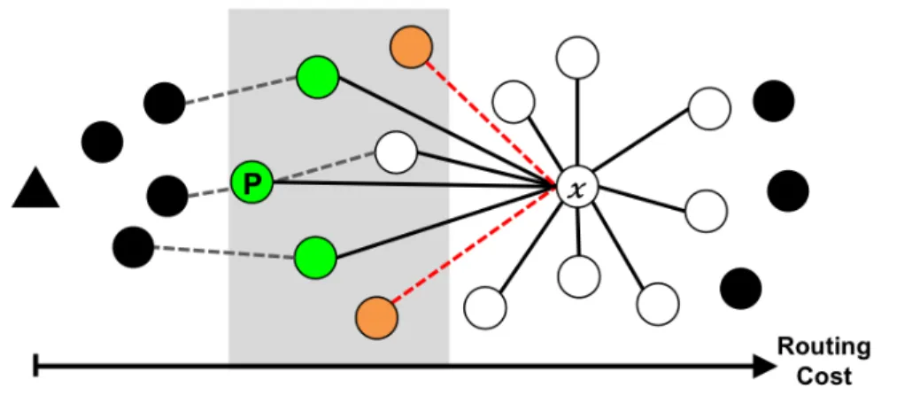
4.1 An example of the parent set of a sending node x with primary parent
node P. . . 35
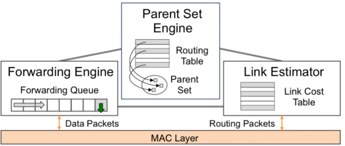
4.2 Main components of CTP+EER. . . 37
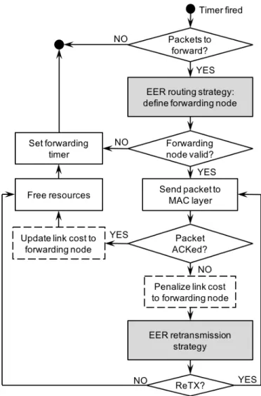
4.3 General flowchart of the packet forwarding process in CTP+EER. . . . 39
4.4 An example of a routing cost inconsistency in EER without relaxing the
Figure Page
4.5 A general illustration of the subtrees of descendants where the largest
blue subtree is the worst case built in CTP (solid lines) for neighbors of the sink. Dashed lines represent additional links used in CTP+EER that
distribute the traffic out of the original subtree in CTP. . . 45
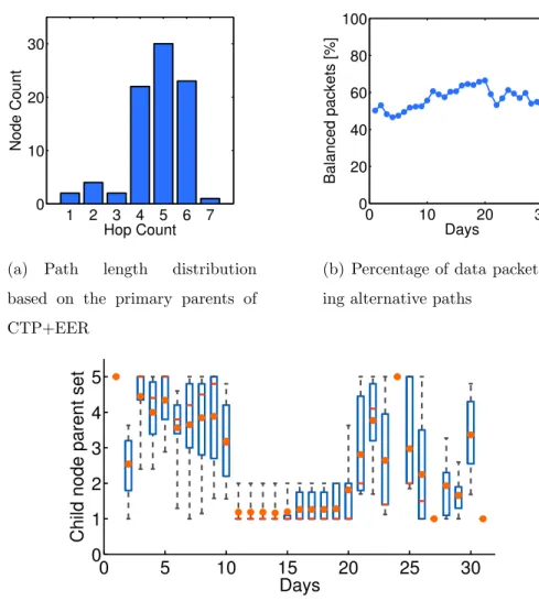
5.1 Path length distribution in Indriya based on CTP. . . 52
5.2 Results from experiments in Indriya. . . 54
5.3 Representation of the network topology of experiments using CTP+EER in Indriya. . . 56
5.4 Improvement of the transmission cost and duty cycle in CTP+EER com-pared to CTP in simulations with random topologies in Cooja. . . 60
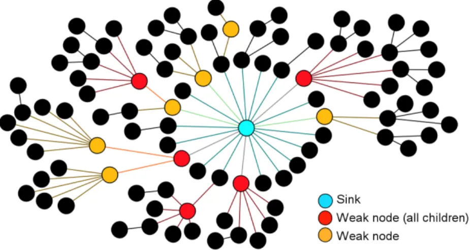
5.5 Results from the evaluation of CTP+EER in the ASWP testbed. . . . 64
5.6 Location of the 84 WSN nodes in the ASWP WSN testbed as of August 2015. Weak nodes diagnosed by CTP+EER are highlighted in orange. 66 6.1 Data packet generation for an IRIS node with ADCs enabled on the MDA300 acquisition board: (1) no external sensors (top); (2) two exter-nal soil moisture sensors (middle); (3) three exterexter-nal soil moisture sensors (bottom). . . 74
6.2 Traffic characteristics of selected nodes from the ASWP testbed. Gener-ated data packets (Ge), forwarded/received data packets (Fw), data packet retransmissions (rTx), routing packet transmissions (cTx), and routing packet receptions (cRx). Daily average values are presented. . . 77
6.3 Energy profiles and duty cycles of selected nodes at ASWP. Daily average values are presented for the following application states: data sampling, data transmissions (DataTx), data receiving+forwarding (RxFw), data retransmission (ReTx), routing transmissions (ctlTx), routing receptions (ctlRx), idle listening, and sleeping. . . 78
6.4 Results obtained for nodes in a laboratory experiment. Daily average values are presented. Drivers are enabled in these nodes, but the external sensors are not attached. They use two AA batteries of the same reference as nodes at ASWP. . . 80
7.1 An illustration of the management system general architecture. . . 84
7.2 INDAMS layered architecture. . . 87
7.3 INDAMS components view. . . 89
Figure Page
7.5 Graphical representation of function categories at the UGL for a generic
client/server scenario. . . 91
7.6 Data model for user access control in INDAMS. . . 92
7.7 Simplified state transition diagram of an agent. . . 95
7.8 Simplified state transition diagram of the server. . . 96
7.9 Implementation example of the agent-server communication via web ser-vices. . . 97
7.10 Multiple clients trying to monitor the same WSN. The data collection function (orange) goes through the UGL and it is executed only once for each WSN. The data monitoring function does not go through the UGL and each client receives the collected data. . . 98
7.11 Operations of the data handler. . . 99
7.12 An illustration of INDAMS for WSN topology monitoring in a residential backyard. . . 101
7.13 INDAMS web interface for agent selection. . . 102
7.14 An example of the agent functions available for the ASWP testbed. . . 103
7.15 Topology monitoring for the ASWP testbed. . . 103
7.16 Data monitoring for the ASWP testbed. . . 105
7.17 Topology monitoring and status of nodes at the ASWP testbed with 84 nodes. Node colors indicate their batteries levels: charged (green), de-pleted (gray), and close to be dede-pleted (orange). . . 106
7.18 Web interface of the database query and export function in INDAMS. . 107
7.19 Web interface of the last received packet function in INDAMS. . . 108
7.20 Web interface for the data indicator function in INDAMS. . . 108
ABSTRACT
Navarro Pati˜no, Miguel A. PhD, Purdue University, May 2016. Energy Efficiency in
Data Collection Wireless Sensor Networks. Major Professor: Yao Liang.
This dissertation studies the problem of energy efficiency in resource constrained
and heterogeneous wireless sensor networks (WSNs) for data collection applications
in real-world scenarios. The problem is addressed from three di↵erent perspectives:
network routing, node energy profiles, and network management. First, the energy
efficiency in a WSN is formulated as a load balancing problem, where the routing layer
can diagnose and exploit the WSN topology redundancy to reduce the data traffic
processed in critical nodes, independent of their hardware platform, improving their energy consumption and extending the network lifetime. We propose a new routing strategy that extends traditional cost-based routing protocols and improves their
energy efficiency, while maintaining high reliability. The evaluation of our approach
shows a reduction in the energy consumption of the routing layer in the busiest nodes ranging from 11% to 59%, while maintaining over 99% reliability in WSN data
collection applications. Second, a study of the e↵ect of the MAC layer on the network
energy efficiency is performed based on the nodes energy consumption profile. The
resulting energy profiles reveal significant di↵erences in the energy consumption of
WSN nodes depending on their external sensors, as well as their sensitivity to changes
in network traffic dynamics. Finally, the design of a general integrated framework and
data management system for heterogeneous WSNs is presented. This framework not only allows external users to collect data, while monitoring the network performance and energy consumption, but also enables our proposed network redundancy diagnosis and energy profile calculations.
CHAPTER 1. INTRODUCTION 1.1 Motivation
Advances in semiconductor technologies allow electronic devices, with a given computing capacity, to decrease their size and cost at an exponential rate, following Moore’s law. Researchers have been able to use these semiconductor-manufacturing techniques for building smaller and inexpensive radios, sensors, and actuators, which enable new possibilities for instrumenting and interacting with the physical world [1]. Wireless sensor networks (WSNs) integrate these low-cost, low-power, and multi-functional devices, presenting a promising approach for various sensing and actuating tasks in multiple application domains.
Unlike traditional networks, WSNs are formed from resource-constrained devices, with limited processing capacity, memory, communication bandwidth, and energy sources [2]. These distinctive characteristics allow new applications but also intro-duce new challenges, unique to sensor networks, compared to other kinds of wireless networks. First, resource limitations are substantial at the node level. For this reason, protocols and algorithms running in WSNs must involve node cooperation to overcome such limitations. Moreover, programs executing in WSN nodes must comply with memory constraints, and therefore, WSN applications require complex design approaches, i.e., operating systems customized for the needs of each particular application [3] [4].
WSNs are envisioned to operate at high scales in terms of size (i.e., number of nodes) and deployment time. Low hardware costs facilitate the acquisition of WSN nodes, not to mention all of them need not use the same components or sensors. In consequence, protocols and WSN applications must be designed considering a high number of nodes and hardware heterogeneity.
WSNs have been used in a variety of applications, e.g., military surveillance, forest fire detection, industrial automation, environmental monitoring, health applications, among others [5] [2]. In general, these applications can be classified into two major
categories: data collection and object detection/tracking. Data collection applications
involve periodic sensing and are designed to sample and transmit their sensor data at defined time intervals. This category normally includes applications with low duty cycles and high network lifetime. The second category corresponds to object de-tection/tracking applications. These applications are designed for reacting after an external event, i.e., forest fire or intrusions, and thus their first objective is detection followed by tracking the event behavior. These processes usually involve active
coor-dination between WSN nodes, and therefore, this category follows a very di↵erent
approach compared to data collection applications. For object detection and track-ing, faster sampling rates are expected and accuracy is often preferred at the expense of higher energy consumption. This classification is not absolute and there are multi-ple scenarios in which WSN applications require incorporating behaviors from both categories.
1.2 Wireless Sensor Networks for Data Collection
This dissertation is focused on WSNs for data collection, which have emerged as a promising alternative to traditional data-collection mechanisms (i.e., data loggers
and sensing stations) enabling cost-e↵ective implementations in various sciences and
engineering domains. In this context, WSN nodes are typically deployed outdoors in harsh environments, which pose great challenges for multi-hop WSN deployments.
WSN nodes are battery powered and thus energy availability is a significant res-trictive factor, in addition to hardware heterogeneity and memory, computing, and bandwidth limitations. In some cases, energy constraints in WSN nodes can be mitigated by the use of energy harvesting mechanisms [6] [7] [8], whereas in many other situations WSN deployments have to rely on batteries as their main energy
source [9] [10] [11] [12] [13] (e.g., due to space constraints, limited sun exposure),
presenting an urgent need for energy efficiency.
Previous studies have attempted to address these energy efficiency issues based
on cross-layer designs [14] [15], limiting their practical applications because of the complexity of re-implementing and replicating the original cross-layer dynamics in
other hardware platforms. Likewise, studies oriented towards energy efficient MAC
layer implementations face similar challenges in the presence of heterogeneous WSN nodes.
The evaluation of WSN protocols and applications also provide some challenges,
as di↵erent implementations cannot be tested under the exactly same real-world and
complex environment. Up to date, di↵erent methods have been used to approach
these challenges, including theoretical model formulations, simulations, emulations, and experimental testing. Theoretical models enable the mathematical derivation of general or asymptotic conditions; although in these cases environment dynamics are often simplified to avoid excessive model complexity. A similar drawback is presented in simulations, where even though the same environment can be used to evaluate multiple approaches, it corresponds to a modeled environment that cannot capture the complex dynamics of real scenarios. Emulations go one step further by allow-ing to evaluate both algorithms and implementations simultaneously, but still un-der simplified environment conditions. Additional information can be obtained from experiments in WSN motes, e.g., using publicly available WSN testbeds; however, real-world deployments are also required for validating data collection applications targeting outdoor environments. Such real-world experiments consider all factors involved in these deployments, which can be easily omitted in any of the previous scenarios. In this dissertation, theoretical models, simulation/emulation, as well as indoor and outdoor testbed experiments are used throughout the validations.
1.3 Major Contributions
This dissertation studies the problem of energy efficiency in resource constrained
and heterogeneous WSNs for data collection applications in real-world scenarios. This
problem is addressed from three di↵erent perspectives: network routing, node energy
profiles, and network management.
First, the energy efficiency problem is formulated as a load balancing problem
where the routing layer can exploit the network redundancy o↵ered by the WSN
topology to reduce the data traffic processed in critical nodes, improving the energy
consumption and network lifetime. This approach is independent of the hardware
platform and reduces the data traffic load on critical nodes by carefully
introduc-ing suboptimal paths, which results in an overall cost-e↵ective solution that extends
traditional cost-based routing protocols, without routing overhead. In addition, the resulting routing strategy is able diagnose nodes with low network redundancy, allow-ing network administrators to correct these situations improvallow-ing the network energy
efficiency and also preventing network partitions in the event of battery depletion or
node failures. The evaluation of our approach shows a reduction in the energy con-sumption of the routing layer in the busiest nodes ranging from 11% to 59%, while maintaining over 99% reliability in data collection applications
Then, a study of the e↵ect of the MAC layer on the network energy efficiency is
performed by analyzing the energy consumption profiles of WSN nodes in real-world scenarios. This approach combines health and instrumentation information from de-ployed WSN nodes with electric current measurements for each state of the WSN
application, reflecting the e↵ect of the external environment and network
dynam-ics. Such measurements can be obtained in a laboratory beforehand for a specific MAC layer implementation, and thus energy profiles can be directly analyzed on
WSN deployments. The resulting energy profiles reveal significant di↵erences in the
their sensitivity to changes in network traffic dynamics, resulting in higher energy consumption.
Finally, the design and implementation of an integrated framework for network and data management in WSNs is presented. This framework systematically supports heterogeneous WSNs under a unified management system and separates management from application functionalities. Furthermore, by processing the health and instru-mentation data collected from WSNs, the framework enables the above mentioned network redundancy diagnosis, as well as the energy profile calculations. This infor-mation is available to network administrators who can take appropriate actions to prevent undesired network behaviors, or react to specific events.
1.4 Organization
This dissertation is organized as follows. Chapter 2 describes the background on WSNs for data collection. Chapter 3 introduces our outdoor WSN testbed
deploy-ment. Chapter 4 presents our new energy efficient and balanced routing strategy and
its implementation. Chapter 5 shows the evaluation of this routing strategy and a case study of its deployment in a real-world outdoor WSN testbed. Chapter 6 presents the construction and analysis of the energy profiles. Chapter 7 gives the design and im-plementation of the framework for network and data management. Finally, Chapter 8 presents the summary of the current work and outlines the future work.
CHAPTER 2. BACKGROUND
As our work is focused on practical WSNs, this chapter introduces the necessary tools for developing data collection WSN applications. It presents the operating system that is used in this dissertation, followed by the standard implementation of routing and MAC layers.
2.1 TinyOS
TinyOS [4] is the most widely used operating system for WSNs. It defines a component-based framework, where WSN applications select a subset of components to build an application-specific operating system into each application. Applications in TinyOS use the NesC language [16], and their typical size is of a few kilo bytes, of which the operating system base is around 400 bytes in RAM.
The components that define a TinyOS program are connected through interfaces,
and use the following computational abstractions: commands, events, and tasks.
Re-quests of services between components are performed throughcommands (e.g.,
trans-mit a data packet), and the corresponding completion of the service is signaled with anevent (e.g., transmission done).
For increasing the system responsiveness, TinyOS allows components to defer time
consuming computations usingtasks. Tasks constitute functions that are executed by
the TinyOS scheduler at a later time following a run-to-completion execution model. Therefore, tasks can perform background computation and cannot be preempted by other tasks, although they can still be preempted by asynchronous code (i.e., interrupt handlers, commands and events).
The amount of work carried by components and events is reduced through
signal (i.e.,events) are decoupled. In this way, a command can post a task with long-running operations and return immediately. Later, the TinyOS scheduler executes the task and once the task finishes an event is signaled.
Throughout this dissertation TinyOS v2.1.2 is used. Other operating systems for WSNs include Contiki [17], RIOT [18], and OpenWSN [19].
2.2 The Collection Tree Protocol
The collection tree protocol (CTP) [20] [21] is the de-facto standard routing pro-tocol for WSNs. It is designed to maintain a robust operation in data collection WSN applications, while promptly reacting to topology changes. The protocol combines three techniques: (1) it uses a link estimator for computing the link quality to neigh-bor nodes, using information from both data and routing packets; (2) CTP uses the
Trickle algorithm [22] for timing routing packets and adapting to di↵erent network
conditions; and (3) CTP performs datapath validation for detecting and recovering routing loops.
CTP is a cost-based routing protocol that aims to compute the best available path from a WSN node to a sink. In the protocol, cost information is disseminated using routing packets and path computations are performed in an iterative manner, as in distributed distance-vector routing protocols, using the expected number of transmissions (ETX) [23] as cost metric. ETX values are associated to links (i.e.,
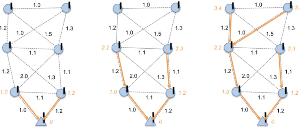
link ETX) and nodes (i.e., node ETX), where the ETX of a node corresponds to the sum of link ETX values in the best path towards the sink, and the sink node has a default ETX equal to zero. An example of the iterations to compute node ETX values in CTP is shown in Figure 2.1, where nodes located one hop from the sink compute their costs based on their link qualities, knowing that the sink has a node ETX equal to zero. In the next iteration, nodes two hops from the sink compute their node costs and the process continues until all nodes in the network define their node ETX values.
a 1.0 1.2 1.1 1.2 2.0 1.3 1.1 1.1 1.2 1.0 1.0 1.5 1.3 0 1.0 1.2 1.1 1.2 2.0 1.3 1.1 1.1 1.2 1.0 1.0 1.5 1.3 0 1.2 1.0 1.0 1.2 2.2 2.3 1.0 1.2 1.1 1.2 2.0 1.3 1.1 1.1 1.2 1.0 1.0 1.5 1.3 0 1.2 1.0 2.2 2.3 3.4 3.3
Figure 2.1. An example of the iterations to compute the node ETX in CTP.
The architecture of CTP defines three major components: Link Estimator,
Rou-ting Engine, andForwarding Engine. These components run on each sensor node and they are connected through multiple interfaces. The Link Estimator computes and maintains the link cost of neighbor nodes. The link ETX is computed taking into account both inbound and outbound link qualities, which are then passed through an exponential smoothing filter. Inbound link quality is computed based on routing packets and outbound link quality is based on data packet transmissions and their acknowledgements. The Routing Engine controls routing packet transmissions based on the Trickle algorithm [22]. It manages the routing table with node ETX values, and it is also in charge of selecting the parent node. The Forwarding Engine is in charge of forwarding data packets, either generated by the sending node or received from its neighbors. It controls data packet retransmissions and indicates the Link Estimator when to update the outbound link quality in the event of packet loss. It also performs loop detection, identifying packets received from nodes with lower ETX as inconsistencies. When this occurs, new routing packets are requested from neighbor nodes, through the Routing Engine, to update the local information before attempting to forward data packets.
PHY MAC Header CTP Data Header App. Payload MAC Footer 10 Bytes 8 Bytes 2 Bytes
ETX!
Origin Node ID!
Sequence Number Collection ID!
P C Reserved (not used) THL!
0 … 8 … 16 bits
Figure 2.2. CTP data packet structure.
Packet Structures
Data Packets: the structure of a generic data packet is presented in Figure 2.2. Physical and MAC-layer headers add a fixed overhead to every data packet trans-mission. In addition, the MAC layer also appends a 2-Byte footer used for error
detection. Following the MAC-layer header, there is theCTP data header (8 Bytes),
and then, the application data payload is introduced.
The CTP data header defines the Pull (P) and Congestion (C) flags. The re-maining 6 bits of the first byte are not specified and they are reserved for future
usage. The second byte includes the Time Has Lived (THL) metric, which works as
a hop counter. Third and fourth bytes defines the ETX of the sending node, which
is used for loop detection. This value is updated after each hop until the sink node is
reached. The node ID of the original sending node is included in the origin node ID
field on bytes fifth and sixth. The byte in position seven contains the CTP sequence
number for data packets. Finally, the eighth byte defines the collection ID value, which indicates the instance of CTP intended to handle the current data packet, as multiple collection services may be initialized from the application layer [24].
Routing Packets: these packets include specific headers controlled by the Link Estimator and Routing Engine components, as shown in Figure 2.3. The routing packet structure shows that a fixed-size header from the Link Estimator (2 Bytes) and a CTP routing header (5 Bytes) are included. After these, there is a variable-size
0""""""""""""""""""…"""""""""""""""""""""8"""""""""""""""""""…""""""""""""""""""16"bits PHY"""MAC"Header""""LE"Header""""CTP"Routing"Header"""LE"Footer"""MAC"Footer Num."Entries"""""""""LE"Seq."Num. P""C""""Reserved"""""""""""Parent"ID Parent"ID"""""""""""""""Node"ETX Node"ETX Link"ETX"1 Node"ID"1 Link"ETX"2 Node"ID"2 Link"ETX"15 Node"ID"15 0""""""""""""""""""…"""""""""""""""""""""8"""""""""""""""""""""""""""""""""""""""""…""""""""""""""""""""""""""""""""""24" bits …"""""""""""""""""""""""""""""… 0""""""""""""""""""…"""""""""""""""""""""8"""""""""""""""""""…""""""""""""""""""16"bits
Figure 2.3. CTP routing packet structure.
footer from the Link Estimator, which may be from 0 to 45 Bytes. Routing packets are processed by the MAC and physical layers in the same way as data packets, and therefore, they also incur in the same header and footer overheads.
The header from the Link Estimator defines two bytes. The first byte is used for coding the number of elements that will be added into the Link Estimator footer,
and the second byte defines the LE sequence number, which is used for computing
the inbound link quality.
The CTP routing header requires five bytes in routing packets. The first byte defines the same entries as the CTP data header described earlier. In addition, the
remaining 4 bytes are used for specifying the parent ID of the current node (2 Bytes)
and the node ETX (2 Bytes) (i.e., path ETX through the parent node).
Finally, the footer from the Link Estimator defines neighbor node ID - link ETX
pairs, which are appended to routing packets depending on the number of neighbors.
Link ETX values in this footer indicate the link cost from the sending node to the neighbor node.
2.2.1 Main Components
This section provides a more detailed description of the implementation of CTP components in TinyOS, based on [21] [24] [25].
Link Estimator
The implementation of CTP available in TinyOS uses the 4-bit link quality esti-mator [26]. The Link Estiesti-mator (LE) component introduces a header and a footer in routing packets, and it also provides the required interfaces to the Routing Engine and Forwarding Engine components. All values computed in the LE component are
stored in aneighbor table, di↵erent from the routing table maintained by the Routing
Engine.
For computing the link ETX value to each neighbor, both transmission (i.e., out-bound) and reception (i.e., inout-bound) link qualities are considered. Transmission
qual-ity is based on data packet transmissions (dataP kttx) and the acknowledgments
re-ceived for these packets (dataP ktack), as defined in (2.1). These values are used after
a specific number of data packets are transmitted to complete a predefined packet window.
Qtx = dataP kttx
dataP ktack (2.1)
Reception quality is computed based on the number of routing packets received from each neighbor. As shown in (2.2), reception quality is defined as the ratio
between the number of routing packets received (routingP ktsrx) and the total number
of routing packets sent from a neighbor node (routingP ktstx). Each node advertises
the number of routing packets transmitted using the LE sequence number field in
routing packets (see Figure 2.3). Similar to transmission quality, reception quality is also used after a specific number of beacons are received from a neighbor node. Before calculating the link ETX, the reception quality estimate is passed through an exponential smoothing filter, averaging new values with previous samples weighted
with an exponentially decaying function [24]. The reception quality estimate used for computing the link ETX is shown in (2.3) and the default value of the decay factor
is 0.9.
Qrx = routingP ktrx
routingP kttx (2.2)
Qrx[t] =↵routingP ktrx
routingP kttx + (1 ↵)Qrx[t 1] (2.3)
Finally, the link ETX for a specific neighbor is computed as defined in (2.4), where
Q represents either transmission or reception quality estimates. As a result, the link
ETX value is updated every time a new transmission or reception quality estimate is
available, using another exponential smoothing filter with default decay factor of 0.9.
LinkET X =↵Q+ (1 ↵)LinkET Xold (2.4)
Routing Engine
As mentioned above, the Routing Engine (REng) in CTP is in charge of handling routing packets, selecting the parent node and maintaining the routing table. The time interval for routing packets is managed based on the Trickle algorithm [22], which basically doubles the time interval after each routing packet transmission until a maximum threshold is reached. CTP defines three possible causes for resetting the Trickle timer:
• Pull bit: when nodes have no routes (e.g., after booting), they set the Pull bit in the CTP header (see Figure 2.2 and Figure 2.3). In response, when nodes receive a packet with the Pull bit set, they reset their Trickle timer and thus
routing traffic increases allowing nodes to establish new routes.
• Routing Loops: when a routing loop is detected by the Forwarding Engine component, it also triggers a Trickle timer reset. By resetting his Trickle timer,
the node detecting a loop sends more frequent routing packets and other nodes in the loop will be able to update their routing information. More about routing loops will be discussed with the Forwarding Engine component.
• ETX changes: when a node detects a sudden improvement in its node ETX value greater than a threshold, it resets its Trickle timer, triggering new route updates and informing neighbor nodes about this improvement. The default
threshold is 2.0.
One additional condition for resetting the Trickle algorithm was defined in [27]. The condition defines that any node in the network can reset their Trickle timer if they receive a routing packet from a neighbor node with a very high node ETX (e.g., higher than 10). In the event of temporary network partitions, data packet retransmissions and routing loops will cause the node ETX from disconnected nodes to increase continuously in a very short time period. Since connected nodes are not experiencing any of the previous three conditions, their Trickle timer will continue to increase exponentially, delaying the opportunity for neighbor nodes to reconnect to the network. By resetting the Trickle timer when high node ETX values are detected from neighbors, nodes that were temporarily disconnected will be able to rejoin the collection tree faster. Similar to the previous condition, this also corresponds to an
efficiency optimization, which allows CTP to react faster to topology changes, unlike
the first two conditions, which are necessary for correctness [21].
The REng in CTP implements the following conditions for selecting a new parent node:
• If the current parent node is congested and the path ETX through a neighbor
node is strictly lower than the sending node ETX (i.e., path ETX through the current parent), plus a threshold of 1.0, then the neighbor node is selected as a new parent node. This condition is presented in (2.5) and it indicates that the new parent node is selected avoiding children from the current node. However,
this condition is never used because congestion has not been implemented in CTP for TinyOS.
• If the path ETX through a neighbor node plus a parent-switch threshold is
strictly less than the node ETX (i.e., path ETX through the current parent), then the neighbor node is selected as the new parent. By default, the
parent-switch threshold in CTP for TinyOS is 1.5, and this condition is presented in
(2.6).
parentcongested & (P athET XbestN eighbor < N odeET X+ 1.0) (2.5)
P athET XbestN eighbor+ 1.5< N odeET X+LinkET XtoP arent (2.6)
Forwarding Engine
All data packets generated by the application layer or received from neighbor nodes are handled by the Forwarding Engine (FEng). First, packets are inserted into a forwarding queue, where they are processed in a first-come, first-served basis. To this end, the FEng retrieves the ID of the current parent from the REng, then, the FEng requests an acknowledgement and passes the data packet to the MAC layer. If the acknowledgement is received after the packet transmission, the data packet is removed from the queue; otherwise, the FEng triggers a CTP retransmission.
CTP retransmissions are performed independently of any MAC-layer retransmis-sions. After a packet acknowledgement is lost, the FEng asks the REng to re-compute routes. This process triggers a new parent selection procedure, but it does not neces-sarily reset the Trickle timer, unless one of the previous conditions is met. Then, the
FEng activates a back-o↵timer and retries sending the data packet to the MAC-layer.
This process is repeated until a maximum number of retransmissions is reached, in which case the data packet would be discarded. The default maximum number of retransmissions in CTP is 30 attempts.
Routing loops in CTP are detected based on inconsistencies of the node ETX values. For the FEng, an inconsistency occurs in data packets received from neighbor nodes, if the received node ETX is lower or equal than the node ETX of the current node. In this case, the FEng triggers a Trickle reset in the REng, generating new routing packets. Moreover, the FEng does not drop looping packets. Instead, it introduces a delay before attempting to forward the packet, allowing other nodes to fix their routes before the transmission. Allowing packets to traverse multiple loops also intends to incrementally repair the network topology and if loops are rare events, then the cost of looping packets would remain low [21].
An additional feature of the FEng is duplicate packet control. Duplicate packets
are identified based on their Origin ID, Collection ID, CTP Sequence Number and
THL. By adding the THL value, CTP is only considering 1-hop duplicates and avoids
discarding looping packets. The FEng maintains a cache of default size 4, which stores the last successfully transmitted packets.
2.3 Low Power Listening (LPL)
TinyOS provides a MAC layer abstraction that implements an asynchronous low power listening (LPL) strategy to duty cycle the radio, reducing the energy consump-tion in WSN nodes [28]. In LPL, nodes sleep most of the time and periodically wake up to sample the wireless channel for activity. When energy is detected, nodes stay awake to receive incoming packets, or they go back to sleep after a predefined timeout interval. In this strategy, most of the work is performed by sending nodes, since nodes
in the network know each otherswakeup interval, but they do not know their wakeup
times. Therefore, to guarantee that the intended receiving node is able to hear the
packet transmission, the sending node needs to transmit during the entire wakeup
interval [29].
TinyOS implements BoX-MAC [30] for LPL, which uses a continuous transmission of the data packet for the duration of the wakeup interval, replacing preamble
trans-2 1 3 4 6 5 Node+A Node+B Node+C
Data$Tx Rx Idle$list. Ack Tx
LPL_DEF_LOCAL_WAKEUP DELAY_AFTER_RECEIVE
Figure 2.4. An example of BoX-MAC in TinyOS for a data packet transmission from node A to node B.
missions used in previous LPL definitions. In this way, both sending and receiving nodes can save additional energy, as receiving nodes are now able to quickly identify packets destined to them and go back to sleep if necessary, while sending nodes can finish a data packet transmission early if an acknowledgement is received before the wakeup interval is completed. Figure 2.4 shows an example of BoX-MAC in TinyOS
for a data packet transmission from node A to node B. The figure indicates di↵erent
events as follows: (1) node B wakes up periodically to sample the wireless channel; (2) node A starts a data packet transmission with node B as destination; (3) node C wakes up, detects activity in the channel, and receives the data packet from A, which
is quickly discarded after verifying that a di↵erent node is the destination; (4) node
B wakes up and receives the data packet from A; (5) node B sends the corresponding packet acknowledgement, node A receives it and finishes the data packet transmis-sion; (6) after sending the packet acknowledgement, node B continues listening the channel for a short time in case more packets were being transmitted.
Parameters that need to be controlled by the LPL implementations in TinyOS
are the local wakeup interval (LPL DEF LOCAL WAKEUP), the neighbors’ wakeup
inter-val (LPL DEF REMOTE WAKEUP), and the time a receiving node will continue listening
after receiving the data packet (DELAY AFTER RECEIVE), as seen in Figure 2.4. All
sleeping nodes in the network configure their local wakeup interval equal to their neighbors’ wakeup interval, while nodes that must remain awake (e.g., sink) set their
local wakeup interval to zero. Other important parameters include the time a send-ing node waits for a packet acknowledgement (i.e., time interval between consecutive packet transmissions as seen in the second event of Figure 2.4), the time that nodes spend sampling the wireless channel, and the time a node requires to receive and process a packet acknowledgement. The proper configuration of these timing param-eters is critical, since if nodes do not spend enough time sampling the channel, they may wake up and go back to sleep while the sending node is still waiting for packet acknowledgments, resulting in unnecessary packet retransmissions. Likewise, if the sending node does not wait long enough between consecutive packet transmissions, it may miss the packet acknowledgement, resulting in unnecessary retransmissions and duplicate packets. It is also important to note that the time required to receive a packet acknowledgement depends on each specific hardware platform, increasing the complexity of heterogeneous WSNs.
TinyOS has two di↵erent architectures for LPL: the default LPL implementation
and the rfxlink implementation. The default LPL implementation is available for
the CC2420 driver in tos/chips/cc2420/. It controls the time that a node
sam-ples the channel with the number of clear channel assessment (CCA) samsam-ples defined
by the parameter MAX LPL CCA CHECKS. On the other hand, the rfxlink
implemen-tation aims to provide a general architecture of the transceiver driver. It controls
the LPL parameters with the LowPowerListeningConfig interface. The RF230 is
one of the transceivers with a driver directly developed using the rfxlink
archi-tecture. The CC2420 transceiver also has a driver with this architecture available in
tos/chips/cc2420x/; however, unstable behaviors were observed in preliminary tests
CHAPTER 3. THE ASWP TESTBED
This chapter introduces the WSN testbed deployment that defines the objective sce-nario of our work with preliminary performance results.
3.1 Deployment
The testbed is deployed at the Beechwood Farms Nature Reserve (BFNR) of the Audubon Society of Western Pennsylvania (ASWP), located in Fox Chapel in north-ern Allegheny County, Pennsylvania, USA, as shown in Figure 3.1. The BFNR is 134 acres of protected land, which is owned by the Western Pennsylvania Conservancy.
Figure 3.1. Location of the ASWP testbed (red dot) in Allegheny County (highlighted in cyan and enlarged), Pennsylvania, USA.
The ASWP testbed was initially deployed in 2010 [31] and since then it has been operating with the objective of exploring the feasibility and challenges of using WSNs for collecting reliable long-term hydrological data and investigating the impacts of vegetation heterogeneity and soil properties on the status and trends of soil moisture and transpiration. Table 3.1 summarizes representative WSN deployments reported in
the past decade, specifying their deployment analysis time, network size, deployment environment, platform, and main application category.
The hardware in the testbed combines heterogeneous WSN platforms and all nodes perform both networking and sensing tasks in a flat network setting (i.e., non-hierarchical deployment). As of August 2015, the ASWP testbed includes 84 WSN nodes, which correspond to 35 TelosB, 25 MICAz, and 24 IRIS motes, with one IRIS sink node. TelosB motes incorporate the 2.4 GHz CC2420 transceiver and the MSP430 microcontroller with 10 KB of RAM. MICAz motes have the same CC2420 transceiver as TelosB motes, and an ATmega128L microcontroller with 4 KB of RAM. The IRIS platform uses the 2.4 GHz RF230 transceiver, and the ATmega1281 micro-controller with 8 KB of RAM. It should be noted that the RF230 transceiver of IRIS motes has a higher maximum output power of 3 dBm, compared to 0 dBm in the CC2420 transceiver of TelosB and MICAz motes.
Figure 3.2. Examples of node configurations in the ASWP testbed. A node hanging from a tree without external sensors (left) and a node mounted onto a PVC pipe with external sensors attached (right).
The BFNR landscape and facility present unique challenges for the deployment of WSN nodes. Internet access is only available at the BFNR Nature Center, while the locations of interest to install the sensors are around 300 m away or farther. In
Ta b le 3. 1. C h ar ac te ri st ic s of re la te d WS N d ep lo y m en ts De pl o ym e n t A n al y si s Ti m e S iz e E n v ir on m e n t P lat for m A p p li c at ion M ot eLab [32] N/A 190 No d es In d o or s T M ot e S k y Ap p . te st in g K an se i G en ie [33] N/A 700 n o d es In d o or s XS M ,T el os B ,I m ot e2 Ap p . te st in g In d ri ya [34] N/A 139 n o d es In d o or s T el os B Ap p . te st in g S en sLab [35] N/A 256x 4 n o d es In d o or s W S N430 Ap p . te st in g F lo ck Lab [36] N/A 30 n o d es In d o or s IR IS ,T el os B ,O p al ,T in y Ap p . te st in g Vi gi lNe t [37] d ay s 70 n o d es O u td o or s/op en ar ea M IC A2 T rac k in g/d et ec ti on E x S cal [38] 15 d ay s 1200 n o d es O u td o or s/op en ar ea M IC A2, XS M T rac k in g/d et ec ti on G re en O rb s [12] 29 d ay s 330 n o d es O u td o or s/f or es t T el os B D at a col le ct ion S NF [7] 30 d ay s 57 n o d es O u td o or s/f or es t M 2135 D at a col le ct ion R ed w o o d s [10] 44 d ay s 33 n o d es O u td o or s/t re e M IC A2D ot D at a col le ct ion S en sor S cop e [6] 2 m on th s 97 n o d es (16 ou td o or s) O u td o or s/gl ac ie r T in y No d e D at a col le ct ion T ri o [39] 4 m on th s 557 n o d es O u td o or s/op en ar ea T ri o M ot e T rac k in g/d et ec ti on G D I [9] 4 m on th s 98+ 49 n o d es O u td o or s M IC A2D ot D at a col le ct ion LUYF [40] 147 d ay s 10 n o d es O u td o or s M IC Az D at a col le ct ion AS W P > 1 y ear 84 n o d es O u td o or s/f or es t M IC Az ,I R IS ,T el os B D at a col le ct ion
addition, the aesthetics of the nature reserve must be maintained, and thus, there are limited locations available where WSN nodes can be placed, especially in areas closer to the Nature Center. For this purpose, the node enclosures were camouflaged and discretely located either hanging from tree branches or mounted onto PVC pipes, as seen in Figure 3.2. Sink Relay node Regular node 50 m N Nature Center
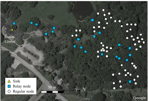
Figure 3.3. Location of the 84 WSN nodes in the ASWP WSN testbed as of August 2015.
Such location restrictions define a network topology where the sink is located in one end and the network grows in a single direction, almost in a conical shape, where the first hops have very low density and the number of nodes increases as we move farther from the sink, as seen in Figure 3.3. As mentioned above, all WSN nodes in the testbed perform sensing tasks; however, not all nodes can be placed in the locations of interest, since some nodes need to build the path from there to the sink.
Nodes are classified based on their sensor configurations into two categories: relay
voltage, temperature, and humidity, and they are mainly used for connecting the lo-cations of interest to the sink node located at the nature center. On the other hand,
regular nodes are equipped with di↵erent configurations of external sensors (e.g., soil
moisture, water potential, sap flow, soil temperature), in addition to the on-board sensors (i.e., voltage, temperature, and humidity), and provide the core of the en-vironmental data. In MICAz and IRIS motes, external sensors are connected using the MDA300 data acquisition board, while TelosB motes use a custom-made board to satisfy the voltage requirements of the external sensors. From the 84 WSN nodes in the ASWP testbed, there are 21 relay nodes and 63 regular nodes, where TelosB and MICAz motes are mainly used as regular nodes, and IRIS motes are preferred as relay nodes.
Figure 3.4. Limited sun exposure in locations of interest at the ASWP testbed.
In addition, the locations of interest present very limited sun exposure for WSN nodes as seen in Figure 3.4, where the tree canopy in the forested area covers most of the field, and thus, WSN nodes in the ASWP testbed remain battery powered.
Since the initial testbed deployment, di↵erent battery types and configurations have
been used, aiming to balance budget limitations, space constraints (e.g., size of the enclosure), maintenance, and performance. As a result, as of August 2015, relay nodes are equipped with three D NiMH rechargeable batteries with 10,000 mAh nominal capacity, considering that they have more space available in their enclosures and
they are mostly deployed closer to the sink to forward the data from their neighbors. Regular nodes are equipped with thee AA NiMH rechargeable batteries with 2,700 mAh nominal capacity.
3.2 Preliminary Performance Analysis
During the first years the ASWP testbed operated using XMesh, Crossbow’s com-mercial mesh networking protocol. XMesh provides a self-healing and self-organizing networking service [41]. The application code for XMesh is compiled specifically for a mote type (e.g., MICAz) and sensor board (e.g., MDA300). Arguments for program-ming the transmission frequency and node/group identifiers are also available. The
ASWP testbed deployment uses the low power (LP) mode, where motes power o↵
non-essential electronics when idle and still forward messages from neighbor motes. For MICAz and IRIS motes, XMesh does not support time synchronization. There-fore, all packet transmissions are made asynchronously.
XMesh’s multi-hop routing is based on the Minimum Transmission (MT) cost metric aiming to minimize the total energy consumed to transmit a packet to the base station [42], similar to CTP which is based on the ETX cost metric. One of the
most important di↵erences in the design of these protocols is that XMesh employs
a fixed Route Update Interval (RUI) for routing packets, while CTP adopts the Trickle algorithm to adapt the frequency of routing packets according to the network conditions, as described earlier in this chapter. Unfortunately, the source code of XMesh is not provided and then it is not possible to examine specific details of its implementation. In the ASWP testbed, XMesh was configured in LP mode with the RUI set to 128 seconds, and using an inter-packet interval (IPI) of 15 minutes.
After the summer of 2013, XMesh was replaced by an open-source approach using the original version of CTP and LPL available in TinyOS 2.1.2. The application was configured with an IPI of 15 minutes, a wakeup interval of 1 second, and a maximum Trickle interval of 60 minutes, while other parameters used default values. In addition,
the application was developed to include the necessary health and instrumentation information in order to study the performance of the protocol.
The information of the datasets used to analyze the protocols is shown in Table
3.2, and the main indicator corresponds to the packet reception rate (PRR), defined
for each node as the ratio between packets received at the sink and the number of generated packets.
Table 3.2.
Datasets for preliminary analysis
Protocol Time Period Active Nodes
XMesh March 2012 - August 2012 42 nodes
CTP November 2013 - April 2014 47 nodes
Figure 3.5 shows a summary of the results obtained from XMesh during the com-plete time period. The PRR for each active node and the network average are shown in Figure 3.5(a). It can be seen that overall XMesh has a low performance with a network PRR of 36.01%, where some nodes located farther from the sink can have PRRs of 27%. In addition to the low reliability in XMesh, it is observed that only a few critical nodes across the network are forwarding most of the data packets, as seen
in Figure 3.5(b). In particular, multi-hop traffic is concentrated in a single node in the
first two hops of the network. Data packet retransmissions are shown in Figure 3.5(c),
and it can be seen that nodes with higher data traffic loads are incurring in higher
retransmissions, evidencing low link quality and limitations of the routing protocol to overcome such situations. Table 3.3 shows the network average PRR of XMesh during the best month within the initial time period, reflecting that although there is a small improvement, the routing protocol still experiences the same limitations observed during the complete time period.
Figure 3.6 shows the results obtained from CTP. In this scenario, higher PRRs are observed for nodes closer to the sink; however, the network PRR is 79.04%, a low
Node ID 0 1001 1010 1020 1030 1040 1050 1060 1070 1080 1091 1100 1110 2003 2015 2025 2030 2045 2055 2065 2071 2085 2095 2103 2115 2125 2135 2141 2150 3005 3015 3025 3035 3045 3055 3065 3075 3085 3095 3105 3113 3125 3130 0 20 40 60 80 100 PRR [%] (a) XMesh PRR. 0 1001 1010 1020 1030 1040 1050 1060 1070 1080 1091 1100 1110 2003 2015 2025 2030 2045 2055 2065 2071 2085 2095 2103 2115 2125 2135 2141 2150 3005 3015 3025 3035 3045 3055 3065 3075 3085 3095 3105 3113 3125 3130 Node ID 0 1000 2000 3000 4000 Forwarded packets
(b) XMesh forwarded packets.
0 1001 1010 1020 1030 1040 1050 1060 1070 1080 1091 1100 1110 2003 2015 2025 2030 2045 2055 2065 2071 2085 2095 2103 2115 2125 2135 2141 2150 3005 3015 3025 3035 3045 3055 3065 3075 3085 3095 3105 3113 3125 3130 Node ID 0 2000 4000 6000 8000 10000 Retransmissions (c) XMesh retransmissions.
Figure 3.5. Summary of results obtained from XMesh at the ASWP testbed during the complete time period. Daily averages are shown for each node, solid lines indicate the network average, and node IDs are sorted based on their distance to the sink.
Table 3.3.
Network average PRR of XMesh and CTP
Protocol PRR (Complete time period) PRR (Best month)
XMesh 36.01% 42.16%
CTP 79.04% 92.71%
value for data collection applications, specially considering that there are still nodes
with very low PRRs under 50%. Similar to XMesh, when using CTP, data traffic
concentration is observed in critical nodes across the network, which are forwarding
most of the data packets. In this case, traffic concentration is higher in critical nodes,
as all other nodes forward very few or zero data packets. Figure 3.6(c) shows a more even distribution of packet retransmissions for all nodes in the testbed, critical and non-critical nodes, showing that CTP is able to correctly identify the best paths in
the network. However, by concentrating the data traffic in the best routing paths,
CTP is also increasing the energy consumption of those critical nodes, reducing their
lifetime and creating more frequent network partitions. The e↵ect of these network
partitions is reflected in the higher PRR achieved by CTP in a shorter time period, as shown in Table 3.3.
These results do not intend to present a direct comparison between the two routing
protocols, but to reflect two states of the testbed with di↵erent configurations to be
0 10011 10101 10201 10301 10401 10501 10601 10701 10801 10911 11001 11101 20031 20151 20251 20301 20451 20551 20651 20711 20851 20951 21031 21151 21251 21351 21411 21501 30051 30151 30251 30351 30451 30551 30651 30751 30851 30951 31051 31131 31251 31301 40031 40051 40131 40151 40231 40251 40331 40351 50031 50131 50231 50331 50431 50531 Node ID 0 20 40 60 80 100 PRR [%] (a) CTP PRR. 0 10011 10101 10201 10301 10401 10501 10601 10701 10801 10911 11001 11101 20031 20151 20251 20301 20451 20551 20651 20711 20851 20951 21031 21151 21251 21351 21411 21501 30051 30151 30251 30351 30451 30551 30651 30751 30851 30951 31051 31131 31251 31301 40031 40051 40131 40151 40231 40251 40331 40351 50031 50131 50231 50331 50431 50531 Node ID 0 1000 2000 3000 4000 Forwarded packets (b) CTP forwarded packets. 0 10011 10101 10201 10301 10401 10501 10601 10701 10801 10911 11001 11101 20031 20151 20251 20301 20451 20551 20651 20711 20851 20951 21031 21151 21251 21351 21411 21501 30051 30151 30251 30351 30451 30551 30651 30751 30851 30951 31051 31131 31251 31301 40031 40051 40131 40151 40231 40251 40331 40351 50031 50131 50231 50331 50431 50531 Node ID 0 100 200 300 400 500 Retransmissions (c) CTP retransmissions.
Figure 3.6. Summary of results obtained from CTP at the ASWP testbed during the complete time period. Daily averages are shown for each node, solid lines indicate the network average, and node IDs are sorted based on their distance to the sink.
CHAPTER 4. ENERGY EFFICIENT AND BALANCED ROUTING (EER)
Cost-based WSN routing protocols [25] [21] have become the de facto standard for
multi-hop data collection applications, and their principles have also been adopted by the IETF Roll working group standard RPL [43]. However, one major drawback of cost-based WSN routing protocols is that they tend to concentrate most of the
data traffic on specific nodes that provide the best available routes. As a result, the
energy consumption across the network is highly unbalanced and the busiest nodes
end up depleting their batteries much faster than their neighbors, removing the best available routes first, and potentially partitioning the network.
To address this problem, we present Energy Efficient Routing (EER), a new
rou-ting strategy for data collection WSNs, which exploits the WSN topology redundancy based on a controlled randomized approach without any additional routing overhead.
EER, based on the concept ofparent set, allows to select suboptimal paths in routing,
reducing the data traffic load on the busiest nodes, resulting in an overall cost-e↵ective
solution that extends the network lifetime. This improvement is achieved by leverag-ing on the establishment of a stable routleverag-ing topology, but replacleverag-ing the best forwarder
with a random selection from theparent set, defined as the subset of neighbor nodes
that provide feasible routing progress towards the sink(s). Consequently, all neighbor nodes included in the parent set share the responsibility of packet forwarding, instead of a single parent node.
EER is aimed for battery-powered multi-hop WSNs for data collection, and focuses
on the energy efficiency and balance achieved by therouting layer, which can certainly
be further complemented by the energy efficiency of the MAC layer, while maintaining
high reliability. Therefore, our approach can be applied to many di↵erent kinds of
cost-based routing solutions, including those implemented as cross-layer optimizations to further improve their network lifetimes.
To demonstrate the proposed EER, we implement it based on the Collection Tree
Protocol (CTP) [21], forming a new routing protocol calledCTP+EER. We validate
CTP+EER against the state-of-the art routing protocols CTP and Opportunistic
Routing in WSNs (ORW) [44], and evaluate their reliability and energy efficiency in
detail.
The specific contributions of this work are:
• We present EER, a new routing strategy that self-adapts to network
condi-tions without the need of complicated configuration parameters, providing an
energy efficient and balanced alternative for practical data collection WSN
de-ployments. Relying on the concept of parent set, EER exploits the suboptimal network routing alternatives in WSNs, and also provides a new diagnosis mech-anism that identifies nodes with strong or weak network redundancy.
• We develop CTP+EER, which extends CTP with our proposed routing strategy
EER. In our implementation, the original CTP provides resource management logic and link quality estimations, while all routing logic is now controlled by EER.
• We formulate the analytical performance model for cost-based routing
pro-tocols (e.g., CTP) and their EER extensions (e.g., CTP+EER). Specifically, we provide the redundancy conditions of the network topology that guarantee
CTP+EER to improve the energy efficiency at the routing layer in comparison
with CTP.
4.1 Related Works
WSN routing protocols for data collection have been proposed and compared based
on bandwidth utilization, reliability, latency, and energy efficiency, where CTP [21] is
often used as the benchmark protocol. Protocols like BCP [45], BRE [46], and Arbu-tus [47] are mainly concerned about improving bandwidth utilization, increasing the
total amount of traffic supported by the network, while maintaining high reliability.
These works operate on high-power conditions and thus address di↵erent scenarios
than those in energy constrained data collection applications, which are the main focus of our work.
ORW [44] presents an opportunistic routing protocol for data collection
applica-tions in WSNs. The opportunistic component in ORW improves the energy efficiency
of duty-cycled implementations by reducing preamble times in low power transmis-sions. While our work also considers multiple nodes as potential forwarders, our parent set considers link quality more strictly for possible parents and excludes nodes
at the same level as the sending node, avoiding potential routing loops that a↵ect the
overall protocol performance, as we will discuss in the chapter. In addition, unlike ORWs forwarder set, we introduce an explicit construction of the parent set, enabling the examination of the topology redundancy for network diagnosis, while remaining a sender-based approach leveraging on cost-based routing mechanisms. In our work, CTP+EER is evaluated versus ORW since in both protocols the contributions of
the routing layer to the total energy efficiency can be clearly di↵erentiated from the
contributions of the MAC layer.
Other works like Dozer [14] and LWB [15] have opted for cross-layer implemen-tations, which tightly couple the behavior of routing and MAC layers. Dozer imple-ments a basic cost-based routing protocol on top of a locally synchronized TDMA-based MAC layer. On the other hand, LWB coordinates fast network floods TDMA-based on global synchronization and scheduling. Cross-layer implementations present ad-ditional challenges when they need to be implemented in multiple platforms (e.g., MICAz, TelosB, IRIS). For instance, the protocol stack needs to be re-implemented and communication parameters need to be re-configured accordingly for each new
platform to replicate the desired cross-layer behaviors when using di↵erent hardware.
An example would be when a WSN node from one platform requires longer time to acknowledge data packets, in which faster platforms would have to consume addi-tional energy for idle listening in order to avoid unnecessary packet retransmissions.
EER di↵ers from these cross-layer solutions in that it concentrates on the energy effi -ciency and balance achieved by the routing layer, while the main factors contributing to lower energy consumption in Dozer and LWB correspond to the MAC layer (i.e., time synchronization and scheduling). Authors of [48] present BFC, a combination of a routing protocol that removes routing packets with an adaptive LPL
implemen-tation. However, it is not clear how much contribution to the total energy efficiency
in BFC comes from the MAC layer and/or routing layer. In addition, we consider
that key energy efficiency factors from Dozer, LWB, and BFC are complementary
to our work, since EER can be implemented on top of MAC layers that support time synchronization, scheduling, or adaptive LPL. Similarly, EER can be applied to cost-based approaches such as Dozer and BFC to further improve their network lifetimes.
Another category of related works is multipath routing, considering that with EER
consecutive data packets may travel through di↵erent paths under a given WSN
topol-ogy. However, the existing WSN multipath routing aims to achieve higher reliability and lower delay in data transmissions either by forwarding packets over multiple paths simultaneously, at the cost of increasing the network energy consumption [49] [50], or by using alternative paths as a backup in the event that the initial path fails [51] [52].
Our approach di↵ers from these works because we use alternative routes as a
proac-tive and consistent routing strategy for energy efficiency and balance, rather than
reacting to a failed path event. RPL [43] defines a subset of neighbor nodes (also named a parent set) as potential parents for data collection and whenever the current best parent node fails, a new best parent node is selected from this candidate set, similar to [51] [52]. In summary, these multipath routing protocols and RPL do not focus on load balancing, incurring in higher energy consumption.
A recent approach named ORPL-LB is presented for load balancing in WSNs in [53]. It adapts the nodes’ wakeup interval to control the number of potential for-warders based on an opportunistic extension of RPL. Nevertheless, ORPL-LB still has the same drawbacks of ORW because its duty cycle adaptation runs on top of
the original forwarder set which may include nodes that create routing loops. Other works on load balancing for WSNs mainly rely on one of the following methods: topology control, clustering, or adding an additional term into the routing cost func-tion [54]. Topology control and clustering mechanisms are not directly relevant to our work, since they focus more on dense networks or require WSN nodes with spe-cial hardware components [55] [56]. Solutions that add a load balancing term into the routing cost function are proposed in [57] and [58] based on estimations of the
energy available on WSN nodes, and in [47] based on the traffic processed by each
node. The main drawback in these works is that defining the weight of the added load balancing term depends on each specific network scenario, and therefore, it requires
a complex configuration process. Our work takes a di↵erent approach where the load
balancing e↵ect is determined by the WSN routing topology itself, without the need
of additional configuration parameters. Moreover, works that rely on energy estima-tions must consider hardware dependent factors such as battery capacity, chemistry, age, number of charging cycles, type of sensors in WSN nodes, and environmental
factors such as temperature and humidity, which introduce high variability a↵ecting
energy estimations and making this kind of methods difficult to use in practical WSN
deployments.
Probabilistic approaches have been reported based on random walks [59] [60], which traded load balancing for higher energy consumption. Another probabilistic approach is presented in [61], where the routing protocol forwards packets to random nodes from the CTP routing table, following a distribution based on routing costs. However, this method has the issue of forwarding packets to the opposite of the cost gradient direction (i.e., forwarding packets to child nodes), which increases the
number of hops, routing loops, and routing packets, and also a↵ects the total energy
consumption.
Finally, optimization-based approaches have also been reported [62] [63] [64]; how-ever, most of these works introduce assumptions not practical in real scenarios (e.g.,