Modelling of a post-combustion CO
2capture process using
extreme learning machine
Fei Li1• Jie Zhang1•Eni Oko2•Meihong Wang2
Received: 21 August 2016 / Revised: 13 January 2017 / Accepted: 13 February 2017 / Published online: 23 February 2017
The Author(s) 2017. This article is published with open access at Springerlink.com
Abstract This paper presents modelling of a post-combustion CO2capture process using bootstrap aggregated extreme
learning machine (ELM). ELM randomly assigns the weights between input and hidden layers and obtains the weights between the hidden layer and output layer using regression type approach in one step. This feature allows an ELM model being developed very quickly. This paper proposes using principal component regression to obtain the weights between the hidden and output layers to address the collinearity issue among hidden neuron outputs. Due to the weights between input and hidden layers are randomly assigned, ELM models could have variations in performance. This paper proposes
combining multiple ELM models to enhance model prediction accuracy and reliability. To predict the CO2production rate
and CO2capture level, eight parameters in the process were utilized as model input variables: inlet gas flow rate, CO2
concentration in inlet flow gas, inlet gas temperature, inlet gas pressure, lean solvent flow rate, lean solvent temperature, lean loading and reboiler duty. The bootstrap re-sampling of training data was applied for building each single ELM and then the individual ELMs are stacked, thereby enhancing the model accuracy and reliability. The bootstrap aggregated extreme learning machine can provide fast learning speed and good generalization performance, which will be used to
optimize the CO2capture process.
Keywords CO2capture Neural networksData-driven modellingExtreme learning machine
1 Introduction
Greenhouse emissions (GHE), mainly carbon dioxide
(CO2), is identified as the chief reason resulting in the
global climate change, especially the global warming. The growing energy demand, due to rapid increasing population and development of industrialization, are directly linked to the increasing release of GHE. The target of a 50%
reduction of CO2 emission by 2050 comparing with the
level in 1950 is set by the Intergovernmental Panel on Climate Change.
Carbon capture and storage (CCS) has been widely
believed as an advanced technology to achieve CO2emission
reduction, which captures, transports and stores CO2. There
are three major types of technologies applied for CCS: post-combustion, pre-combustion and oxyfuel combustion. Among these various CCS technologies, post-combustion
CO2capture (PCC) process is considered as the most
con-venient way to reduce CO2emission from coal fired power
plants, as it can retrofit the exiting power plant and be inte-grated into new ones. However, PCC process will generate a large amount of energy penalty, which reduces the efficiency and effectiveness of the power plant. The energy requirement is strongly influenced by the operation conditions, equip-ment dimensions and capture target of PCC process. Therefore, it is necessary to apply process optimisation in order to enhance the efficiency of CCS systems.
& Jie Zhang
1 School of Chemical Engineering and Advanced Materials,
Newcastle University, Newcastle upon Tyne NE1 7RU, UK
2 Department of Chemical and Biological Engineering,
University of Sheffield, Sheffield S1 3JD, UK DOI 10.1007/s40789-017-0158-1
In order to optimize the operation of post-combustion
CO2capture process, a reliable and accurate process model
is necessary. In the past, researchers have proposed various kinds of modelling technologies, such as mechanistic
models (Lawal et al.2010; Biliyok et al.2012; Posch and
Haider2013; Cormos and Daraban2015) and data-driven
models (Zhou et al.2009,2010; Sipocz and Assadi2011).
However, some problems have been raised up by using the above mentioned methods. For instance, the development of mechanistic model is not only time consuming, but also needs a huge volume of knowledge of the underlying first principles of the process. It is also computationally very demanding when using a detailed mechanistic model in process optimisation. Statistic models can overcome these problems and are efficient in building data driven models, but they still have a few shortcomings. It is shown in that statistical model is unable to describe the nonlinear rela-tionships that possibly exits among the parameters (Zhou
et al. 2010). In this case, another advanced modelling
method, artificial neural networks (ANNs), is proposed to address the above weakness. However, feedforward neural networks trained by the back propagation (BP) learning algorithm have some issues: firstly, the most appropriate learning rate is difficult to determine; secondly, the pres-ence of local minima affects the modelling results; then, networks would possibly be over trained leading to poor generalization performance; lastly, it is also time-con-suming when applying gradient based learning (Huang et al.2006).
Extreme learning machine (ELM) was proposed into address the issue of slow training in conventional
feed-forward neural networks (Huang et al. 2006). ELM is
basically a single hidden layer feedforward neural network with randomly assigned weights between the input and hidden layers. The weights between the hidden and output layers are determined in a one-step regression type approach using generalised inverse. Thus, an ELM can be built very quickly. As the weights between the input and hidden layers are randomly assigned, correlations can exist among the hidden neuron outputs and variations in model performance can exist. This paper proposes using principal component regression (PCR) to obtain the weights between the hidden and output layers in order to overcome the correlation issue among hidden neuron outputs. This paper also proposes building multiple ELMs on bootstrap re-sampling replications of the original training data and then combining these ELMs in order to enhance model accuracy and reliability. The proposed method is applied to the dynamic model development of the whole post-combustion process plant.
This paper is structured as follows: Sect.2 briefly
pre-sents post-combustion CO2 capture process through
chemical absorption. Extreme learning machine, a method
for calculating output layer weights in ELM using PCR,
and aggregating multiple ELM are given in Sect.3.
Application results and discussions are presented in
Sect.4. Section5draws some concluded remarks.
2 CO
2capture process through chemical
absorption
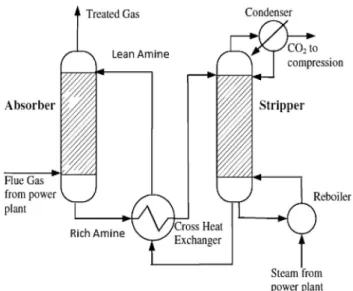
Figure1 shows a typical post-combustion CO2 capture
process through chemical absorption. It consists of two major parts: an absorber and a stripper. In details, the flue gas from the power plant is pressured into the bottom of absorber and contacted counter-currently with lean MEA solution from the top side. The lean MEA solution will
chemically absorb the CO2in flue gas, forming rich amine
solution. The treated gas stream containing much lower
CO2content is leaving from the top of absorber. Then the
rich amine solution is pressured into the regenerator before preheating in the cross heat exchanger. In the stripper, CO2
is separated from rich amine solution by the heat provided
from the reboiler. The regenerated CO2is cooled in
con-denser and compressed for storage, and remaining solution (lean solution) is recycled to the cross heat exchanger to exchange heat with rich amine. The heat supplied in the reboiler, coming from the low pressure steam from power plant, is used to increase the temperature of solution,
sep-arate CO2from rich amine and vaporize the gas in stripper.
This will result in a large energy consumption.
Two parameters are identified to affect the process
performance: CO2capture level and CO2production rate.
CO2capture level is the amount of CO2extracted from the
Fig. 1 Simplified process flow diagram of chemical absorption process for post-combustion capture plant
inlet flue gas in absorber column, which is calculated in Eq. (1).
gco2capture¼1
moutlet co2Voutlet gas minlet co2Vinlet gas
ð1Þ
where,moutlet co2,Voutlet gas, minlet co2 andVinlet gasrepresent
CO2mass fraction in gas out of absorber, gas flow rate out
of absorber, CO2mass fraction in inlet flow gas of
absor-ber, and inlet gas flow rate of absorabsor-ber, respectively.
CO2 production rate represents the amount of CO2
captured after the condenser, which is an indicator for the whole process because it is not affected by a single com-ponent of the process. It is calculated as in Eq. (2):
oco2¼m_co2v~outlet gas ð2Þ whereoco2is CO2production rate after the condenser,m_co2 andv~outlet gasare CO2mass fraction and gas flow rate of the
outlet gas from stripper respectively.
3 Bootstrap aggregated ELM
3.1 Single hidden layer neural networks
Figure2 shows the structure of a single hidden layer
feedforward neural network (SLFN). For Narbitrary
dis-tinct samples (xi,ti), where x¼½xi1;xi2;. . .;xin
T
2Rn is a vector of network inputs andti¼½ti1;ti2;. . .;timT2Rmis a vector of the target values of network outputs. The output
of a standard SLFNs with N˜ hidden nodes and activation
functiong(x) is shown in the following equation:
oj¼
XN~ i¼1
bigiwixjþbi; j¼1;. . .;N ð3Þ
where wi¼½wi1;wi2;. . .;winT is a vector of the weights
between the ith hidden node and the input nodes,biis the
bias of the ith hidden nodes, xj is the jth input sample,
oj=[oj1,oj2,…, ojm]T[ Rmis a vector of the SLFN
out-put corresponding to the jth input sample, bi[ Rm is a
vector of the weight linking the ith hidden node and the
output node. The output node is chosen to have linear activation function and the hidden layer neurons use the sigmoid activation function in this paper.
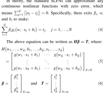
In theory, the standard SLFNs can approximate any continuous nonlinear functions with zero error, which means PNj~¼1 ojtj
¼0. Specifically, there exitsbi, wi
andbito make: XN~ i¼1 bigi wixjþbi ¼tj; j¼1;. . .;N ð4Þ
The above equation can be written asHb=T, where:
H w1;. . .;wN~;b1;. . .;bN~;x1;. . .;xN~ ¼ g wð 1x1þb1Þ g wN~x1þbN~ .. . . . . .. . g wð 1xNþb1Þ g wN~xNþbN~ 2 6 4 3 7 5 NN~ ð5Þ b¼ bT1 .. . bTN~ 2 6 4 3 7 5 ~ Nm and T¼ t1T .. . tT N 2 6 4 3 7 5 Nm ð6Þ
In the above equations,His called hidden layer output
matrix of the neural network and theith column ofHis the
ith hidden node output with respect to inputsx1,x2,…,xN.
Training of SLFNs can be done through finding the
mini-mum value ofE¼minkHNNbNmTNmk.
SLFNs are usually trained by gradient-based learning algorithms, such as BP algorithm, which typically need many iterations and are typically slow. The process of
training is to search the minimum value of
HNNbNmTNm
k k by numerical optimisation
meth-ods. In this procedure, the parameters h =(b, w, b) is
iteratively adjusted as below:
h¼hk1g oEð Þh
oh ð7Þ
where g is the learning rate. By using BP algorithm, the
parameters are updated by error propagation from the output layer to the input layer.
3.2 Bootstrap aggregated ELM
Huang et al. have proved that, if the activation function g(x) is infinitely differentiable in any interval and the number of hidden nodes is large enough, it is not necessary to adjust all the weighting parameters of the network
(Huang et al.2006). In other words, the weights and biases
xj 1 n 1 i Ñ Oj 1 H(w1, b1, x) H(wÑ, bÑ, xÑ) H(wi, bi, xi) βj β1 βÑ m
between the input and hidden layers can be randomly chosen. In order to get good performance, the required number of hidden nodes is not more than the number of input samples. Huang et al. have used a method of finding a
least square solution of the linear equation Hb=T to
obtain the weights between the hidden and output layers.
b¼HyT ð8Þ
whereHyis the generalised inverse ofH.
However, as the hidden layer outputs can be collinear, the modelling performance would be poor by using least square solution to find the weights between the hidden and output layers. This would be especially true for ELM as they have randomly assigned hidden layer weights and typically large number of hidden neurons are required. This paper proposes using PCR to obtain the weights between the hidden and output layers to overcome the
multi-collinearity problems. Instead of regressing H and T
di-rectly, the principal components of Hmatrix are used as
regressors.
The matrix H can be decomposed into the sum of a
series of rank one matrices through principal component decomposition.
H¼u1pT1 þu2pT2 þ þuNpTN ð9Þ In the above equation,uiandpiare theith score vector
and loading vector respectively. The score vectors are orthogonal, likewise the loading vectors, in addition they
are of unit length. The loading vector p1 defines the
direction of the greatest variability and the score vectoru1,
also known as the first principal component, represents the projection of each column ofHontop1. The first principal
component is thus that linear combination of the columns
in H explaining the greatest amount of variability
(u1=Hp1). The second principal component is that linear
combination of the columns in H explaining the next
greatest amount of variability (u2=Hp2) subject to the condition that it is orthogonal to the first principal com-ponent. Principal components are arranged in decreasing
order of variability explained. Since the columns inHare
highly correlated, the first a few principal components can explain the majority of data variability inH.
H¼UkPTkþE¼
Xk i¼1
uipTi þE ð10Þ
whereUk=[u1u2…uk], Pk=[p1p2…pk],k represents
the number of principal components to retain, andEis a
matrix of residuals of unfitted variation.
If the firstk principal components can adequately
rep-resent the original data setH, then regression can be
per-formed on the first k principal components. The model
output is obtained as a linear combination of the first k
principal components of Has
^
T¼Ukw¼HPkw ð11Þ
where w is a vector of model parameters in terms of
principal components.
The least squares estimation ofwis:
w¼ UTkUk
1
UTkT¼ PTkHTHPk
1
PTkHTT ð12Þ
The model parameters in Eq. (8) calculated through
PCR are then given by the following equation: b¼Pkw¼Pk PTkH
THP
k
1
PTkHTT ð13Þ
The number of principal components,k, to be retained in
the model is usually determined through cross-validation
(Wold 1978). The data set for building a model is
parti-tioned into a training data set and a testing data set. PCR models with different numbers of principal components are developed on the training data and then tested on the testing data. The model with the smallest testing errors is then considered as having the most appropriate number of principal components.
As shown in (Zhang 1999; Li et al. 2015), combining
several networks can improve the prediction accuracy on unseen data and give a better generalization performance. The bootstrap re-sampling replication of the original training data is used for training individual networks and the overall output of the aggregated neural networks is a weighted combination of the individual neural network outputs (Fig.3).
Therefore, the procedure of building bootstrap aggre-gated ELM model can be summarized as follows:
Given an activation functiong(x), and number of hidden
nodesN˜,
Step 1: Apply bootstrap re-sampling to produce n (e.g.
n=50) replications of the original training data
set, (xi,ti)1,…, (xi,ti)n,xi2Rn,ti2Rm,i=1,…, N
Step 2: On each bootstrap replication of the original training data, build an ELM model:
Step 2(a): Randomly assign hidden layer
weightswiand biasbi,i=1…N˜
Step 2(b): Calculate the hidden layer output
matrixH
Step 2(c): Calculate the output weights b by
PCR
Step 3: Combine the n (e.g. n =50) ELM models by
averaging their predictions
It has been suggested that, the model prediction confi-dence bounds can be calculated from individual predictions by using bootstrap aggregated neural networks (Zhang
1999; Li et al.2015). The standard error of theith predicted value is calculated as re¼ 1 n1 Xn b¼1 y xi;Wb y xð i;Þ 2 ( )1 2 ð14Þ where y(xi)= P b=1 n y(x
i;Wb)/n and n is the number of
neural networks. The 95% prediction confidence bounds
can be calculated as y(xi;)±1.96re. It indicates a 95%
confidence interval which will contain the true process output with a probability of 0.95. A narrower confidence bound is preferred as it indicates the associated model prediction is more reliable.
4 Performance evaluation
The simulated dynamic process operation data in (Li et al.
2015) were used to build data-driven models. The
simu-lated data were generated from the mechanistic model implemented in gPROMS at University of Hull with a sampling time of 5 s. The data were divided into three groups: training data (56%), testing data (24%), and unseen validation data (20%). Furthermore, the constructed model used the input data of the second batch in which the lean solution flow rate has a step change, to verify its accuracy. To demonstrate the good performance of bootstrap aggre-gated ELM, its results are compared with those from (Li
et al. 2015). Before training, the data should be scaled to
zero mean and unit variance. Both bootstrap aggregated neural network (BA-NNs) and BA-ELM models combine 30 neural networks. In addition, the numbers of hidden neurons used in BA-NNs and BA-ELM are selected within the range of 2–20 and 40–100 respectively. All models with the number of hidden neurons in the above ranges are developed and tested on the testing data. The models give
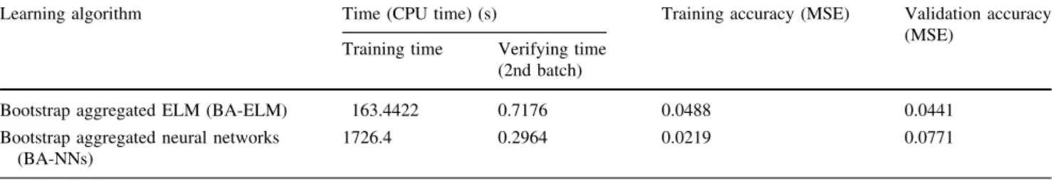
Table 1 Performance comparison of BA-ELM and BA-NNs for CO2production rate
Learning algorithm Time (CPU time) (s) Training accuracy (MSE) Validation accuracy (MSE)
Training time Verifying time (2nd batch)
Bootstrap aggregated ELM (BA-ELM) 163.4422 0.7176 0.0488 0.0441 Bootstrap aggregated neural networks
(BA-NNs) 1726.4 0.2964 0.0219 0.0771 0 50 100 150 200 250 300 350 400 450 500 0 0.01 0.02 0.03 0.04 0.05 0.06 0.07 0.08 time(s)
CO2 production rate(kg/s)
CO2 production rate prediction by BA-ELM
Actual values One-step ahead Multi-steps ahead 0 50 100 150 200 250 300 350 400 450 500 0 0.01 0.02 0.03 0.04 0.05 0.06 0.07 0.08 time(s)
CO2 production rate(kg/s)
CO2 production rate prediction by BA-NNs
Actual value One-step ahead Multi-steps ahead
Fig. 4 Dynamic model prediction of CO2production rate using
the smallest mean squared errors (MSE) are considered as having the appropriate number of hidden neurons. The reason for ELM having more hidden neurons is due to the random nature of hidden layer weights in ELM and small number of hidden neurons would usually not be able to provide adequate function representation. The form of the
dynamic model is shown in Eq. (15).
yðtÞ ¼f y tð ð 1Þ;u1ðt1Þ;u2ðt1Þ;. . .;u8ðt1ÞÞ
ð15Þ
wherey represents CO2 capture level or CO2 production
rate, u1 to u8 are, respectively, inlet gas flow rate, CO2
concentration in inlet flue gas, inlet gas temperature, inlet gas pressure, MEA circulation rate, lean loading, lean solution temperature, and reboiler temperature.
Equa-tion (15) represents a first order nonlinear dynamic model
which is of the lowest order. For practical applications, model of the least complexity is generally preferred. If the low order nonlinear dynamic model could not give
satisfactory performance, then higher order nonlinear dynamic models should be considered.
When developing the two different models, it is clearly seen that BA-ELM model is very simple because its training only needs one iteration. The performance com-parison of the bootstrap aggregated neural networks and
bootstrap aggregated ELM is shown in Table1. The
training CPU time of BA-ELM is about nine times lower than that of BA-NNs. The short training time of BA-ELM is due to the fact that each individual ELM is trained in one step without the need of gradient based iterative training. The verification time of BA-ELM is longer than that of BA-NN as the individual ELMs have more hidden neurons than the individual networks in BA-NN. The MSE value on the unseen validation data from BA-NNs is higher than that from BA-ELM. This could be due to the training of some neural networks in BA-NN might have been trapped in local minima or over fitted the noise. The results given in
Table1 demonstrate that BA-ELM is able to train faster
and perform better than BA-NNs. The performance of one-step ahead predictions and multi-one-step ahead predictions of
CO2production rate in BA-ELM and BA-NNs is indicated
in Fig. 4. Clearly, the prediction using BA-ELM model is
0 5 10 15 20 25 30 35 0 0.02 0.04 0.06 0.08
MSE (training & testing)
Number of neural networks
0 5 10 15 20 25 30 35 0 0.05 0.1 0.15 0.2 MSE (validation)
Number of neural networks
Fig. 5 MSE of CO2production rate for individual ELM models
0 5 10 15 20 25 30 35
0 0.02 0.04 0.06
MSE (training & testing)
Number of neural networks
0 5 10 15 20 25 30 35
0 0.05 0.1
MSE (validation)
Number of neural networks
Fig. 6 MSE of CO2production rate for bootstrap aggregated ELM
0 100 200 300 400 500 600 97.2 97.4 97.6 97.8 98 98.2 98.4 98.6 98.8 99 time(s)
CO2 capture level (%)
CO2 capture level prediction by BA-ELM
Actual value One-step ahead Multi-steps ahead 0 100 200 300 400 500 600 97.2 97.4 97.6 97.8 98 98.2 98.4 98.6 98.8 99 time(s)
CO2 capture level
CO2 capture level prediction by BA-NNs
Actual value One-step ahead Multi-steps ahead
Fig. 7 Dynamic model prediction of CO2capture level using
much better than that using BA-NNs model, especially after 92 steps for the long range prediction.
The MSE values of CO2production rate for individual
ELM models can be seen in Fig.5. The performance on the
unseen validation data is not in accordance with that on the training and testing data. For instance, the prediction on the unseen validation data by the 20th ELM is the worst, however, its performance on the training and testing data is better than many of the individual ELM models. This clearly demonstrates that single network has non-robust nature. Nevertheless, when several individual networks are combined together to build the model, the weakness can be
addressed easily. Figure6 indicates the MSE values on
model building data by aggregating different numbers of
ELM models. The first bar in Fig.6 represents the first
individual ELM model shown in Fig.5, the second bar
represents the combination of the first two individual ELM models, and the last bar represents combining all the individual ELM models. Look into the trends of top and
bottom plots in Fig.6, the prediction performance of
bootstrap aggregated ELM on the unseen validation data is consistent with that on the training and testing data. In other words, combining several ELM models is able to get more accurate predictions on the training and testing data, as well as on the unseen validation data, than single ELM
models. Furthermore, the MSE values in Fig.6 indicates
that, the aggregated ELM model provides more accurate predictions than single ELM models, when comparing with
the MSE values in Fig.5.
Figure7 shows the performance comparison of
one-step-ahead predictions and multi-one-step-ahead predictions of
CO2capture level using BA-ELM and BA-NNs models. It
is clear seen from the bottom graph both one-step-ahead predictions and multi-step-ahead predictions from BA-NN are reasonably accurate though some errors are observable, but the long range predictions (green line) are not accurate after 82 steps (410 s). However, in the top graph, the accurate one-step-ahead predictions and multi-step-ahead predictions from BA-ELM are very encouraging, indicat-ing that the model has captured the underlyindicat-ing dynamics of the process. Such accurate long range predictions can be
further used for model predictive control and real-time optimisation applications.
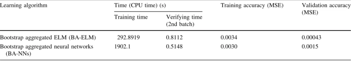
The performance comparison of the bootstrap aggre-gated neural networks and bootstrap aggreaggre-gated ELM for
CO2capture level is shown in Table2. The training CPU
time of BA-ELM is six times lower than that of BA-NN, while its verifying CPU time is a little bit longer than the latter one. This is because each network in the BA-ELM has more hidden neurons than each network in BA-NN. Looking into the comparison of the accuracy, the mean squared error (MSE) values on training data in both models are almost same, while the MSE value of BA-ELM on validation data is three times lower than that of BA-NNs. This shows that BA-ELM has a faster training speed and better generalization performance than BA-NNs, which has
been proved in Huang et al. (2006). The faster training
speed of BA-ELM is due to the ELMs are trained in a one-step procedure without the need of gradient based iterative procedure.
5 Conclusions
The BA-ELMs is demonstrated as a powerful tool to model
the post-combustion CO2 process, which can be trained
much faster and is more accurate than the BA-NNs models. It gives a good generalization performance on unseen data, because the aggregation of multiple ELM can make the model avoid being trapped into local minima and over-fitting problems. As ELM can be trained very quickly without iterative network weight updating, aggregating multiple ELMs does not pose any computational issues in model development. The model will be used to optimize
the CO2capture process in the future. The model prediction
confidence bounds provided by the BA-ELM can be incorporated in the optimisation objective function to
enhance the reliability of the optimisation (Zhang 2004).
Nevertheless, the BA-ELM still exits some problems. For instance, the number of hidden neurons is quite large, which may increase the model computation burden in
Table 2 Performance comparison of BA-ELM and BA-NNs for CO2capture level
Learning algorithm Time (CPU time) (s) Training accuracy (MSE) Validation accuracy (MSE)
Training time Verifying time (2nd batch)
Bootstrap aggregated ELM (BA-ELM) 292.8919 0.8112 0.0034 0.00043 Bootstrap aggregated neural networks
(BA-NNs)
optimisation studies. Further works on BA-ELM will be carried out to address these shortcomings.
Acknowledgements The work was supported by the EU through the project ‘‘Research and Development in Coal-fired Supercritical Power Plant with Post-combustion Carbon Capture using Process Systems Engineering techniques’’ (Project No. PIRSES-GA-2013-612230) and National Natural Science Foundation of China (61673236).
Open Access This article is distributed under the terms of the Creative Commons Attribution 4.0 International License (http://crea tivecommons.org/licenses/by/4.0/), which permits unrestricted use, distribution, and reproduction in any medium, provided you give appropriate credit to the original author(s) and the source, provide a link to the Creative Commons license, and indicate if changes were made.
References
Biliyok C, Law A, Wang MH, Seibert F (2012) Dynamic modelling, validation and analysis of post-combustion chemical absorption CO2capture plant. Int J Greenhouse Gas Control 9:428–445
Cormos AM, Daraban IM (2015) Dynamic modelling and validation of amine-based CO2capture plant. Appl Therm Eng 74:202–209
Huang GB, Zhu QY, Siew CK (2006) Extreme learning machine: theory and applications. Neurocomputing 70(1–3):489–501
Lawal A, Wang M, Stephenson P, Koumpouras G, Yeung H (2010) Dynamic modelling and analysis of post-combustion CO2
chemical absorption process for coal-fired power plants. Fuel 89(10):2791–2801
Li F, Zhang J, Oko E, Wang MH (2015) Modelling of a post-combustion CO2 capture process using neural networks. Fuel
151:156–163
Posch S, Haider M (2013) Dynamic modelling of CO2 absorption
from coal-fired power plants into an aqueous monoethanolamine solution. Chem Eng Res Des 91(6):977–987
Sipocz NTF, Assadi M (2011) The use of artificial neural network models for CO2capture plants. Apply Energy 88(7):2368–2376
Wold S (1978) Cross validatory estimation of the number of components in factor and principal components models. Tech-nometrics 20:397–404
Zhang J (1999) Developing robust non-linear models through bootstrap aggregated neural networks. Neurocomputing 25:93–113
Zhang J (2004) A reliable neural network model based optimal control strategy for a batch polymerisation reactor. Ind Eng Chem Res 43(4):1030–1038
Zhou Q, Chan CW, Tontiwachiwuthikul P, Idem R, Gelowitz D (2009) A statistical analysis of the carbon dioxide capture process. Int J Greenhouse Gas Control 3(5):535–544
Zhou Q, Wu YX, Chan CW, Tontiwachiwuthikul P (2010) Applica-tions of three data analysis techniques for modelling the carbon dioxide capture process. In: 2010 23rd Canadian conference on electrical and computer engineering (Ccece)