Missouri University of Science and Technology Missouri University of Science and Technology
Scholars' Mine
Scholars' Mine
Engineering Management and SystemsEngineering Faculty Research & Creative Works Engineering Management and Systems Engineering 01 Oct 2017
Time Series Classification using Deep Learning for Process
Time Series Classification using Deep Learning for Process
Planning: A Case from the Process Industry
Planning: A Case from the Process Industry
Nijat MehdiyevJohannes Lahann Andreas Emrich David Lee Enke
Missouri University of Science and Technology, [email protected]
et. al. For a complete list of authors, see https://scholarsmine.mst.edu/engman_syseng_facwork/626
Follow this and additional works at: https://scholarsmine.mst.edu/engman_syseng_facwork Part of the Operations Research, Systems Engineering and Industrial Engineering Commons Recommended Citation
Recommended Citation
N. Mehdiyev et al., "Time Series Classification using Deep Learning for Process Planning: A Case from the Process Industry," Procedia Computer Science, vol. 114, pp. 242-249, Elsevier, Oct 2017.
The definitive version is available at https://doi.org/10.1016/j.procs.2017.09.066
This work is licensed under a Creative Commons Attribution-Noncommercial-No Derivative Works 4.0 License. This Article - Conference proceedings is brought to you for free and open access by Scholars' Mine. It has been accepted for inclusion in Engineering Management and Systems Engineering Faculty Research & Creative Works by an authorized administrator of Scholars' Mine. This work is protected by U. S. Copyright Law. Unauthorized use including reproduction for redistribution requires the permission of the copyright holder. For more information, please contact [email protected].
Available online at www.sciencedirect.com
1877-0509 © 2017 The Authors. Published by Elsevier B.V.
Peer-review under responsibility of the scientific committee of the Complex Adaptive Systems Conference with Theme: Engineering Cyber Physical Systems.
10.1016/j.procs.2017.09.066
ScienceDirect
Procedia Computer Science 114 (2017) 242–249
10.1016/j.procs.2017.09.066 1877-0509
Available online at www.sciencedirect.com
ScienceDirect
Procedia Computer Science 00 (2017) 000–000
www.elsevier.com/locate/procedia
1877-0509 © 2017 The Authors. Published by Elsevier B.V.
Peer-review under responsibility of the scientific committee of the Complex Adaptive Systems Conference with Theme: Engineering Cyber Physical Systems.
Complex Adaptive Systems Conference with Theme: Engineering Cyber Physical Systems, CAS
October 30 – November 1, 2017, Chicago, Illinois, USA
Time Series Classification using Deep Learning for Process
Planning: A Case from the Process Industry
Nijat Mehdiyev
a, Johannes Lahann
a, Andreas Emrich
a, David Enke
b,*, Peter Fettke
a, Peter Loos
a a Institute for Information Systems at German Research Center for Artificial Intelligence (DFKI) & Saarland University, Saarbruecken, Germanyb Laboratory for Investment and Financial Engineering, Engineering Management and Systems Engineering, Missouri University of Science and Technology, Rolla, MO, 65409-0370, USA
Abstract
Multivariate time series classification has been broadly applied in diverse domains over the past few decades. However, before applying the classification algorithms, the vast majority of current studies extract hand-engineered features that are assumed to detect local patterns in the time series. Therefore, the efficiency and precision of these classification approaches are heavily dependent on the quality of variables defined by domain experts. Recent improvements in the deep learning domain offer opportunities to avoid such an intensive hand-crafted feature engineering which is particularly important for managing the processes based on time-series data obtained from various sensor networks. In our paper, we propose a framework to extract the features in an unsupervised (or self-supervised) manner using deep learning, particularly stacked LSTM Autoencoder Networks. The compressed representation of the time-series data obtained from LSTM Autoencoders are then provided to Deep Feedforward Neural Networks for classification. We apply the proposed framework on sensor time series data from the process industry to detect the quality of the semi-finished products and accordingly predict the next production process step. To validate the efficiency of the proposed approach, we used real-world data from the steel industry.
© 2017 The Authors. Published by Elsevier B.V.
Peer-review under responsibility of the scientific committee of the Complex Adaptive Systems Conference with Theme: Engineering Cyber Physical Systems.
Keywords: Deep Learning; Time Series Classification; Process Industry; Steel Surface Defect Detection
* Corresponding author. Tel.: 573-341-4749 E-mail address: [email protected]
Mehdiyev, Lahann, Emrich, Enke, Fettke, and Loos / Procedia Computer Science 00 (2017) 000–000
1.Introduction
It is a crucial requirement for manufacturing enterprises to be able to react on certain situations in the market or in the internal production environment in real-time. There is a strong need to leverage the latest big data technologies, novel machine learning and artificial intelligence methods for monitoring, predicting, and thereby improving the manufacturing processes. For this purpose it is necessary to operationalize big data driven predictive analytics by embedding it to the business, operation and manufacturing processes which supports human experts in making critical business decisions by providing actionable insights or acting as a fully automated decision making system [1]. The enterprises can create value only by making the predictive analytics as an integral part of the business processes and operational decisions [2].
The main purpose of process monitoring in the manufacturing environment is identification of abnormalities and faults in process operations. Industrial process monitoring tasks are mainly categorized as (i) fault detection, (ii) fault identification and diagnosis, (iii) estimation of fault magnitudes, and (iv) product quality monitoring and control [3]. The techniques for monitoring the operational processes that rely on diverse analytical methods are classified into three groups: (i) quantitative model based methods, (ii) qualitative model based methods and (iii) process history based or data driven methods [4]. Model based approaches are based on first-principle methods and rely on the concept of residual analysis. They compute the residuals by comparing the estimated values with those of the a-priori known model and detect the anomalies. Although the model based methods are the most reliable approaches for process monitoring, such techniques suffer several disadvantages, as in the majority of cases the analytical description of newly developed complex industrial processes are unavailable and it is a time-consuming issue for domain experts to obtain it.
On the contrary, process history based data-driven approaches don’t require a pre-determined model since the models are obtained from a large amount of available historical process data. As one of the most important data-driven modelling approaches for diverse industrial process monitoring tasks, time series classification has found a broad range of applications in both discrete and process industries. However, current solutions to (multivariate) time series classification problems in the complicated process industry settings appear to be unsatisfactory since they heavily rely on domain experts for extracting the hand-crafted features. The requirements for real-time and immediate processing of stream data from Internet of Things (IoT) networks, and the concept drift which is referred as the evolution of behavior patterns in the sensor data over time, mitigate the effectiveness of conventional feature engineering and machine learning methods. Furthermore, the non-stationary, non-linear and dynamically evolving nature of the sensor data, which serve as valuable input for process monitoring modelling and the necessity to capture temporal relationship in the time series data, demand a novel design of machine learning algorithms. These approaches should satisfy the computational efficiency with a desired level of prediction accuracy and precision.
The present paper aims to propose a multi-stage deep learning to address these challenges in the multivariate time series classification problem for monitoring the product quality in the process industry. The contribution of the present paper is twofold: (i) the application of deep learning technique, particularly the stacked Long-Short Term Memory (LSTM) Autoencoders, to build hierarchical representations from unlabelled multivariate sensor time series data and (ii) the application of deep feedforward neural networks to make the cost-sensitive classifications by incorporating the knowledge by domain experts about the financial consequences of the prediction results. We evaluate the proposed approach in a real-world use case from the steel industry. As a process industry, the steel industry has quite special characteristics when evaluating data spanning the whole steel production process. In our case we attempt to predict the post-processing activities for semi-finished steel products depending on the steel surface quality. For this purpose we consider the sensor data which track various parameters of the steel continuous casting plant throughout the steel casting process and chemical data which describe the chemical compounds added to a steel casting mix based on the product qualities that are planned for an upcoming steel batch.
The remainder of the paper is organized as follows: Section 2 introduces a brief review of the related works for time series classification problems. Section 3 provides an overview to the proposed multi-stage deep learning approach and discusses the LSTM Autoencoder stage for feature extraction and deep feedforward neural networks for classification problem. Section 4 introduces the case study. Section 5 introduces the experiment settings, evaluation metrics and empirical results. Section 6 concludes the paper and discusses the future work.
Nijat Mehdiyev et al. / Procedia Computer Science 114 (2017) 242–249 243 Available online at www.sciencedirect.com
ScienceDirect
Procedia Computer Science 00 (2017) 000–000
www.elsevier.com/locate/procedia
1877-0509 © 2017 The Authors. Published by Elsevier B.V.
Peer-review under responsibility of the scientific committee of the Complex Adaptive Systems Conference with Theme: Engineering Cyber Physical Systems.
Complex Adaptive Systems Conference with Theme: Engineering Cyber Physical Systems, CAS
October 30 – November 1, 2017, Chicago, Illinois, USA
Time Series Classification using Deep Learning for Process
Planning: A Case from the Process Industry
Nijat Mehdiyev
a, Johannes Lahann
a, Andreas Emrich
a, David Enke
b,*, Peter Fettke
a, Peter Loos
a a Institute for Information Systems at German Research Center for Artificial Intelligence (DFKI) & Saarland University, Saarbruecken, Germanyb Laboratory for Investment and Financial Engineering, Engineering Management and Systems Engineering, Missouri University of Science and Technology, Rolla, MO, 65409-0370, USA
Abstract
Multivariate time series classification has been broadly applied in diverse domains over the past few decades. However, before applying the classification algorithms, the vast majority of current studies extract hand-engineered features that are assumed to detect local patterns in the time series. Therefore, the efficiency and precision of these classification approaches are heavily dependent on the quality of variables defined by domain experts. Recent improvements in the deep learning domain offer opportunities to avoid such an intensive hand-crafted feature engineering which is particularly important for managing the processes based on time-series data obtained from various sensor networks. In our paper, we propose a framework to extract the features in an unsupervised (or self-supervised) manner using deep learning, particularly stacked LSTM Autoencoder Networks. The compressed representation of the time-series data obtained from LSTM Autoencoders are then provided to Deep Feedforward Neural Networks for classification. We apply the proposed framework on sensor time series data from the process industry to detect the quality of the semi-finished products and accordingly predict the next production process step. To validate the efficiency of the proposed approach, we used real-world data from the steel industry.
© 2017 The Authors. Published by Elsevier B.V.
Peer-review under responsibility of the scientific committee of the Complex Adaptive Systems Conference with Theme: Engineering Cyber Physical Systems.
Keywords: Deep Learning; Time Series Classification; Process Industry; Steel Surface Defect Detection
* Corresponding author. Tel.: 573-341-4749 E-mail address: [email protected]
Mehdiyev, Lahann, Emrich, Enke, Fettke, and Loos / Procedia Computer Science 00 (2017) 000–000
1.Introduction
It is a crucial requirement for manufacturing enterprises to be able to react on certain situations in the market or in the internal production environment in real-time. There is a strong need to leverage the latest big data technologies, novel machine learning and artificial intelligence methods for monitoring, predicting, and thereby improving the manufacturing processes. For this purpose it is necessary to operationalize big data driven predictive analytics by embedding it to the business, operation and manufacturing processes which supports human experts in making critical business decisions by providing actionable insights or acting as a fully automated decision making system [1]. The enterprises can create value only by making the predictive analytics as an integral part of the business processes and operational decisions [2].
The main purpose of process monitoring in the manufacturing environment is identification of abnormalities and faults in process operations. Industrial process monitoring tasks are mainly categorized as (i) fault detection, (ii) fault identification and diagnosis, (iii) estimation of fault magnitudes, and (iv) product quality monitoring and control [3]. The techniques for monitoring the operational processes that rely on diverse analytical methods are classified into three groups: (i) quantitative model based methods, (ii) qualitative model based methods and (iii) process history based or data driven methods [4]. Model based approaches are based on first-principle methods and rely on the concept of residual analysis. They compute the residuals by comparing the estimated values with those of the a-priori known model and detect the anomalies. Although the model based methods are the most reliable approaches for process monitoring, such techniques suffer several disadvantages, as in the majority of cases the analytical description of newly developed complex industrial processes are unavailable and it is a time-consuming issue for domain experts to obtain it.
On the contrary, process history based data-driven approaches don’t require a pre-determined model since the models are obtained from a large amount of available historical process data. As one of the most important data-driven modelling approaches for diverse industrial process monitoring tasks, time series classification has found a broad range of applications in both discrete and process industries. However, current solutions to (multivariate) time series classification problems in the complicated process industry settings appear to be unsatisfactory since they heavily rely on domain experts for extracting the hand-crafted features. The requirements for real-time and immediate processing of stream data from Internet of Things (IoT) networks, and the concept drift which is referred as the evolution of behavior patterns in the sensor data over time, mitigate the effectiveness of conventional feature engineering and machine learning methods. Furthermore, the non-stationary, non-linear and dynamically evolving nature of the sensor data, which serve as valuable input for process monitoring modelling and the necessity to capture temporal relationship in the time series data, demand a novel design of machine learning algorithms. These approaches should satisfy the computational efficiency with a desired level of prediction accuracy and precision.
The present paper aims to propose a multi-stage deep learning to address these challenges in the multivariate time series classification problem for monitoring the product quality in the process industry. The contribution of the present paper is twofold: (i) the application of deep learning technique, particularly the stacked Long-Short Term Memory (LSTM) Autoencoders, to build hierarchical representations from unlabelled multivariate sensor time series data and (ii) the application of deep feedforward neural networks to make the cost-sensitive classifications by incorporating the knowledge by domain experts about the financial consequences of the prediction results. We evaluate the proposed approach in a real-world use case from the steel industry. As a process industry, the steel industry has quite special characteristics when evaluating data spanning the whole steel production process. In our case we attempt to predict the post-processing activities for semi-finished steel products depending on the steel surface quality. For this purpose we consider the sensor data which track various parameters of the steel continuous casting plant throughout the steel casting process and chemical data which describe the chemical compounds added to a steel casting mix based on the product qualities that are planned for an upcoming steel batch.
The remainder of the paper is organized as follows: Section 2 introduces a brief review of the related works for time series classification problems. Section 3 provides an overview to the proposed multi-stage deep learning approach and discusses the LSTM Autoencoder stage for feature extraction and deep feedforward neural networks for classification problem. Section 4 introduces the case study. Section 5 introduces the experiment settings, evaluation metrics and empirical results. Section 6 concludes the paper and discusses the future work.
244 Mehdiyev, Lahann, Emrich, Enke, Fettke, and Loos / Procedia Computer Science 00 (2017) 000–000 Nijat Mehdiyev et al. / Procedia Computer Science 114 (2017) 242–249
2.Related Work
Time series classification was identified as one of the most challenging 10 problems in the data mining research and has already been investigated for a few decades [5]. The success of the distance based methods, particularly, k-Nearest Neighbor (k-NN) classifiers for time series classifications, have already been documented [6]. The feature based time series classification approaches have also been applied in diverse domains ranging from healthcare to the statistical control of the industrial processes [7]. The main idea of the feature-based classification is the extraction of the discriminative features from the time series data and combining them to make classifications. However, these approaches are based on handcrafted feature engineering and demand intensive pre-processing work. The combination of different approaches such as Dynamic Time Warping + Decision Trees, Dynamic Time Warping + k-NN, and Gaussian Mixture Approaches, among others, have also found their applications in diverse domains [8]. Recently, a few attempts have been made aimed at the application of deep learning approaches for time series classification problems. In their comprehensive review, [9] examined the recent developments in deep learning and unsupervised feature learning for time-series problems. [10] and [11] proposed Convolutional Neural Networks (CNN) based deep learning framework for multivariate time series classification.
3.Proposed Approach
In the present study we proposed a multi-stage deep learning approach to address the classification based on the weakly labeled time series data obtained from multiple sensors. The classification with the weakly labeled data associates the long time series data with a single global class label. This in turn requires one to define the length of the sub-sequences by applying specific algorithms, such as sliding windows. The present study focuses on a predictive monitoring of production processes based on the product quality enabled by IoT networks and information obtained from the chemical analysis. The complicated nature of the problem reduces the effectiveness of handcrafted feature engineering process and demands the implementation of the models which are capable of representing the features from unlabeled data. Therefore, at the first stage of our methodology, we use the stacked LSTM Autoencoders as the baseline unsupervised model to extract the features from the time series data. After performing the necessary data processing stages, including the zero paddings and extracting the features automatically from the raw data with stacked LSTM Autoencoders at the second stage of the proposed approach, the deep feedforward neural networks is applied to perform the classification.
3.1. LSTM Autoencoders
Principal Component Analysis (PCA) is an effective method for reducing the data dimensionality and extracting the features. However, PCA can only model linear interdependencies among the features of the given dataset. Autoencoders are the non-linear generalization of PCA [12]. They are a family of neural networks which are well suited to explore the underlying structure in the dataset in an unsupervised (self-supervised) manner. Autoencoders encode the high dimensional input data to the hidden layers using the relevant activation functions and then try to reconstruct the original inputs through the decoder layer as accurate as possible. They are trained with the backpropagation algorithm with the purpose to minimize the reconstruction loss. Depending on the problem type and complexity various types of autoencoder models, such as simple or deep fully connected autoencoders, convolutional autoencoders, sequence-to-sequence autoencoders (LSTM Autoencoders), contractive autoencoders, and variational autoencoders, among others, can be applied to extract the features.
RNN have been proofed to be effective for many sequence learning tasks like handwriting recognition, speech recognition, and sentiment analysis [13]. Distinguished from other topologies of neural networks, the output of RNN is fed back again to the net along with the next input data. This allows the RNN to remember previous states and learn interdependencies in time series data. However, since RNN are trained using backpropagation, they are affected by the vanishing gradient problem. Each time step in a time series introduces a new layer in the RNN and makes training the network very resource consuming. LSTM networks try to solve this problem by using the gating technique which estimates the relevance of future time steps and ignores irrelevant ones [13]. Since we focus on extracting the features from time series sensor data, we apply stacked LSTM Autoencoders to generate features,
Mehdiyev, Lahann, Emrich, Enke, Fettke, and Loos / Procedia Computer Science 00 (2017) 000–000
which can be later feed to our classification algorithm, as described in the next sub-section. LSTM Autoencoder models have been successfully proposed for sequence-to-sequence learning tasks like machine translation [14], natural language generation and reconstruction [15], and image captioning [16].
For each classification instance, there exist m�-dimensional vectors x��� representing time series data, where � denotes the data source type and x��� describes the number of time steps for data source �. For each data source type � we train a separate LSTM-Encoder x��� as well as an LSTM-Decoder x
��� � ���x��� where n � m�. Reducing the
size of each time series to a constant n, the encoded feature vector of each sensor can just be concatenated and then passed to our classification model. While feeding all sensor data together in one LSTM might allow to reveal dependencies between different sensors this would come with the price of more heavy computations. The LSTM Autoencoders are trained to reconstruct the normal time-series for all steel slabs minimizing the reconstruction loss. However, the decoders are only used to find suitable encoding functions to be applied before the classification task. Figure 1 depicts the aforementioned model.
Fig. 1. Stacked LSTM Autoencoder and deep feedforward neural network 3.2. Deep Feedforward Neural Networks
Both academic and practical applications of deep neural networks have already provided very promising results in many applications from diverse domains [17]. Despite their superiority over the shallow prediction methods, it is a very challenging task to perform the learning on the big data due to complexities in parallelization of learning algorithms [18]. The necessity to overcome the shortcomings related to the learning processes of the traditional neural networks motivated the researchers to innovate diverse algorithmic approaches, such improving the optimizers, exploring novel approaches for parallelization, applying locally connected networks, etc., resulting in groundbreaking studies in the last decade [12], [18].
In the present paper we apply fully connected deep feedforward neural networks to perform the classification based on the features extracted from the previous LSTM Autoencoders. The activation of the neuron through the network is related to the previous one with following formula [19]:
���� ��� �� ��� ������ ���� (1)
where ��� is the activation of the ��� neuron in the ��� layer which is related to the activations in the �� � ���� layer; � is the activation function; ���� is the weight from ��� neuron, and ��� is the bias of the ��� neuron in the ��� layer.
Nijat Mehdiyev et al. / Procedia Computer Science 114 (2017) 242–249 245
Mehdiyev, Lahann, Emrich, Enke, Fettke, and Loos / Procedia Computer Science 00 (2017) 000–000
2.Related Work
Time series classification was identified as one of the most challenging 10 problems in the data mining research and has already been investigated for a few decades [5]. The success of the distance based methods, particularly, k-Nearest Neighbor (k-NN) classifiers for time series classifications, have already been documented [6]. The feature based time series classification approaches have also been applied in diverse domains ranging from healthcare to the statistical control of the industrial processes [7]. The main idea of the feature-based classification is the extraction of the discriminative features from the time series data and combining them to make classifications. However, these approaches are based on handcrafted feature engineering and demand intensive pre-processing work. The combination of different approaches such as Dynamic Time Warping + Decision Trees, Dynamic Time Warping + k-NN, and Gaussian Mixture Approaches, among others, have also found their applications in diverse domains [8]. Recently, a few attempts have been made aimed at the application of deep learning approaches for time series classification problems. In their comprehensive review, [9] examined the recent developments in deep learning and unsupervised feature learning for time-series problems. [10] and [11] proposed Convolutional Neural Networks (CNN) based deep learning framework for multivariate time series classification.
3.Proposed Approach
In the present study we proposed a multi-stage deep learning approach to address the classification based on the weakly labeled time series data obtained from multiple sensors. The classification with the weakly labeled data associates the long time series data with a single global class label. This in turn requires one to define the length of the sub-sequences by applying specific algorithms, such as sliding windows. The present study focuses on a predictive monitoring of production processes based on the product quality enabled by IoT networks and information obtained from the chemical analysis. The complicated nature of the problem reduces the effectiveness of handcrafted feature engineering process and demands the implementation of the models which are capable of representing the features from unlabeled data. Therefore, at the first stage of our methodology, we use the stacked LSTM Autoencoders as the baseline unsupervised model to extract the features from the time series data. After performing the necessary data processing stages, including the zero paddings and extracting the features automatically from the raw data with stacked LSTM Autoencoders at the second stage of the proposed approach, the deep feedforward neural networks is applied to perform the classification.
3.1. LSTM Autoencoders
Principal Component Analysis (PCA) is an effective method for reducing the data dimensionality and extracting the features. However, PCA can only model linear interdependencies among the features of the given dataset. Autoencoders are the non-linear generalization of PCA [12]. They are a family of neural networks which are well suited to explore the underlying structure in the dataset in an unsupervised (self-supervised) manner. Autoencoders encode the high dimensional input data to the hidden layers using the relevant activation functions and then try to reconstruct the original inputs through the decoder layer as accurate as possible. They are trained with the backpropagation algorithm with the purpose to minimize the reconstruction loss. Depending on the problem type and complexity various types of autoencoder models, such as simple or deep fully connected autoencoders, convolutional autoencoders, sequence-to-sequence autoencoders (LSTM Autoencoders), contractive autoencoders, and variational autoencoders, among others, can be applied to extract the features.
RNN have been proofed to be effective for many sequence learning tasks like handwriting recognition, speech recognition, and sentiment analysis [13]. Distinguished from other topologies of neural networks, the output of RNN is fed back again to the net along with the next input data. This allows the RNN to remember previous states and learn interdependencies in time series data. However, since RNN are trained using backpropagation, they are affected by the vanishing gradient problem. Each time step in a time series introduces a new layer in the RNN and makes training the network very resource consuming. LSTM networks try to solve this problem by using the gating technique which estimates the relevance of future time steps and ignores irrelevant ones [13]. Since we focus on extracting the features from time series sensor data, we apply stacked LSTM Autoencoders to generate features,
Mehdiyev, Lahann, Emrich, Enke, Fettke, and Loos / Procedia Computer Science 00 (2017) 000–000
which can be later feed to our classification algorithm, as described in the next sub-section. LSTM Autoencoder models have been successfully proposed for sequence-to-sequence learning tasks like machine translation [14], natural language generation and reconstruction [15], and image captioning [16].
For each classification instance, there exist m�-dimensional vectors x��� representing time series data, where � denotes the data source type and x��� describes the number of time steps for data source �. For each data source type � we train a separate LSTM-Encoder x��� as well as an LSTM-Decoder x
�
�� � ���x��� where n � m�. Reducing the
size of each time series to a constant n, the encoded feature vector of each sensor can just be concatenated and then passed to our classification model. While feeding all sensor data together in one LSTM might allow to reveal dependencies between different sensors this would come with the price of more heavy computations. The LSTM Autoencoders are trained to reconstruct the normal time-series for all steel slabs minimizing the reconstruction loss. However, the decoders are only used to find suitable encoding functions to be applied before the classification task. Figure 1 depicts the aforementioned model.
Fig. 1. Stacked LSTM Autoencoder and deep feedforward neural network 3.2. Deep Feedforward Neural Networks
Both academic and practical applications of deep neural networks have already provided very promising results in many applications from diverse domains [17]. Despite their superiority over the shallow prediction methods, it is a very challenging task to perform the learning on the big data due to complexities in parallelization of learning algorithms [18]. The necessity to overcome the shortcomings related to the learning processes of the traditional neural networks motivated the researchers to innovate diverse algorithmic approaches, such improving the optimizers, exploring novel approaches for parallelization, applying locally connected networks, etc., resulting in groundbreaking studies in the last decade [12], [18].
In the present paper we apply fully connected deep feedforward neural networks to perform the classification based on the features extracted from the previous LSTM Autoencoders. The activation of the neuron through the network is related to the previous one with following formula [19]:
���� ��� �� ��� ������ ���� (1)
where ��� is the activation of the ��� neuron in the ��� layer which is related to the activations in the �� � ���� layer; � is the activation function; ���� is the weight from ��� neuron, and ��� is the bias of the ��� neuron in the ��� layer.
246 Mehdiyev, Lahann, Emrich, Enke, Fettke, and Loos / Procedia Computer Science 00 (2017) 000–000 Nijat Mehdiyev et al. / Procedia Computer Science 114 (2017) 242–249
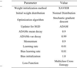
We examine the performance of our networks in different settings using diverse activation functions (see Table 1). The hyperparameter and other advanced optimization parameters of the used deep neural network is presented in Table 2.
Table 1. Non-linear activation functions Table 2. Other Deep Learning Parameters
4. Process Industry: Use Case
The case study in the present paper concentrates on the proactive monitoring of the business and production processes at one of the major German steel producers with the aim to improve the product quality and customer satisfaction. Steel bar production processes are especially utmost important since almost half a million tons of steel are produced in this production facility annually. The variety in chemical properties of steel, the irregularities in the continuous casting processes - which lead to the undesired form of the solidification, and other internal/external and controllable/uncontrollable events may result in the deviations in the product quality especially in steel surface defects. Depending on the type and grade of the surface defects, further processing of steel slabs must be carried out. Therefore, the production experts are required to perform the adaptation of the process instances and an intensive re-planning of production processes in order to meet the customer demands without delays. In the present paper we apply the proposed multi-stage deep learning approach to predict the further processing activities by considering the time series sensor data and chemical properties of the steel.
5. Empirical Results 5.1. Process and Data
In order to understand the used data for our time series classification problem, we provide a very brief description of the continuous casting process. Continuous casting process is the metallurgical process that enables to monitor the transformation of the molten liquid metal to the solid state for producing the semi-finished products. The process starts with the tapping of the molten steel from the ladle to the intermediate container, tundish. The melt with the temperature below 1600° C pours then into the mold through the casting tube. At this phase of the casting the liquid steel gets the solidified shell between the plates of the water-cooled mold. Furthermore, mold casting powder is continuously added to create a slag layer which eliminates the undesired inclusions from the liquid. The upward and downward oscillations of the mold can be observed, which may result in the depressions in the steel slab surface. After leaving the mold phase, the steel with the thin glowing shell is further cooled down with the water along the strand. After getting solidified completely, the cutting of the metal takes place and the slabs as semi-finished products are formed.
Activation Function Plot Equation
Rectified linear unit (ReLU)
���� � ��������� � �������� � �
Leaky rectified linear unit
(Leaky ReLU) ���� � ����1�������� � ����������������� � �
TanH ���� � ����1�������� � ����������������� � �
Exponential Linear Units ���� �� � ������������ � �� 1������� � �
SoftPlus ���� � ����1 � ��)
Softmax ���� �1 � �1��
Parameter Value
Weight initialization method XAVIER Initial weight distribution Normal Distribution
Optimization algorithm Stochastic gradient descent Updater for SGD ADAM ADAMs mean decay 0.9
ADAMs var decay 0.99
Momentum 0.9
Learning rate 0.01 Bias learning rate 0.01 Bias initialization 1.0
Loss Function Multiclass Cross Entropy
Mehdiyev, Lahann, Emrich, Enke, Fettke, and Loos / Procedia Computer Science 00 (2017) 000–000
The values of diverse continuous casting process variables may significantly affect the quality of the slabs. The irregular parameters may lead to the steel surface defects which are as a deviation from the normative appearance, form, size, macrostructure [20]. Cracks, laps, scratches and surface decarburizations are the main steel surface defects. Depending on the degree of these defects, various post-processing activities, such as steel pickling, surface grinding, etc., are required in order to bring the semi-finished products to the designed form. In the current practical applications the steel slabs are inspected visually through a multi-stage process that is very cost intensive. Therefore, in the present study we aim to predict the post-processing activities by considering different parameters obtained from the sensor installed along the strand, such as tundish mass, air ingress, mold level fluctuations, oscillation frequency, mold heat flux, mold water flow, casting speed, casting speed change, etc. We obtain data from 89 sensors that control the values of the different variables in different positions. The size of analyzed sensor data was 3 Terabytes. As mentioned above, we also used the data about the chemical properties of the steel that were strongly assumed to increase the prediction accuracy.
5.2. Tools
The experiments were performed in two phases on two different computers, since the pre-processing stage had different computational requirements than the modeling stage. For the preprocessing phase we used a machine with 6 TB disk space, 64 GB memory and 20 Intel Xeon CPUs E502-2630 v4 with 2.20GZ. As data manipulation software we used Apache Zeppelin on top of a standalone Apache Spark Cluster in a Docker environment [21].
For the creation of the autoencoders, we used a machine with 16 GB memory and two NVIDEA GEFORCE GTX TITAN X. The autoencoders were implemented with the Keras package on top of Tensorflow in python notebooks [22]. The classification with deep feedforward neural networks were performed using the deeplearning4j library [23] on the top the WEKA data mining software [24] in order to be able to perform cost sensitive analysis. 5.3. Evaluation Results
To assess the performance of the proposed model, we used the evaluation metrics tailored to multi-class classification problems [25]. Particularly, we concentrated on two important measures, the average accuracy of the classifier and recall values for each class. The recall, the true positive rate for the particular class, is a very important measure for our case since we aim to avoid the false negatives. To be clear, if the semi-finished products have the surface defects and our model fails to identify them, then it may have undesired consequences - since in this case our predictive model suggests that the no further processing stages are required since steel slabs don’t have any surface problem. Relying on these results and sending the defective products to the customers may have significantly more monetary (also non-monetary) costs than the costs of inspecting the products.
The multivariate time series classification problem for steel quality prediction based on the sensor data is not only complicated due to the irregularities in the input data but also imbalanced structure of the class distribution. In our case almost 85% of the steel slabs had the good quality and no further processing stage was required. The main challenge is identification of the slabs with failures. By applying our multi-stage deep learning classification model directly on the original data, we obtain the average accuracy of 87.49 %. This result can be interpreted positively for relatively balanced datasets (See Table 3). However, a deep look to the recall values of each class reveals that the direct application of the algorithm favors the majority class by getting a recall value 0.994. This value suggests that 99.4% of the steel slabs with good quality were identified by the algorithm. The respective recall values for slabs with surface defects that required steel pickling or surface grinding were 0.026 (for both cases). These results imply that the algorithm could improve the results of the zero (base) model just slightly and was unable to detect the steel products (only 2.6% of them were identified) that require post-processing stages. Despite the obtained high accuracy, the direct application of the model fails to fulfill the requirements of the production managers.
To overcome the problems related to the learning with imbalanced data, a set of diverse (i) data level techniques, (ii) algorithmic level approaches, and (iii) cost-sensitive methods were proposed [26]. The data level methods include randomly oversampling the minority class, randomly undersampling the majority class, informatively oversampling the minority class, informatively undersampling the majority class, and oversampling the small class by generating new synthetic data. The algorithm level approaches investigate the possibilities of adjusting the
Nijat Mehdiyev et al. / Procedia Computer Science 114 (2017) 242–249 247
Mehdiyev, Lahann, Emrich, Enke, Fettke, and Loos / Procedia Computer Science 00 (2017) 000–000
We examine the performance of our networks in different settings using diverse activation functions (see Table 1). The hyperparameter and other advanced optimization parameters of the used deep neural network is presented in Table 2.
Table 1. Non-linear activation functions Table 2. Other Deep Learning Parameters
4. Process Industry: Use Case
The case study in the present paper concentrates on the proactive monitoring of the business and production processes at one of the major German steel producers with the aim to improve the product quality and customer satisfaction. Steel bar production processes are especially utmost important since almost half a million tons of steel are produced in this production facility annually. The variety in chemical properties of steel, the irregularities in the continuous casting processes - which lead to the undesired form of the solidification, and other internal/external and controllable/uncontrollable events may result in the deviations in the product quality especially in steel surface defects. Depending on the type and grade of the surface defects, further processing of steel slabs must be carried out. Therefore, the production experts are required to perform the adaptation of the process instances and an intensive re-planning of production processes in order to meet the customer demands without delays. In the present paper we apply the proposed multi-stage deep learning approach to predict the further processing activities by considering the time series sensor data and chemical properties of the steel.
5. Empirical Results 5.1. Process and Data
In order to understand the used data for our time series classification problem, we provide a very brief description of the continuous casting process. Continuous casting process is the metallurgical process that enables to monitor the transformation of the molten liquid metal to the solid state for producing the semi-finished products. The process starts with the tapping of the molten steel from the ladle to the intermediate container, tundish. The melt with the temperature below 1600° C pours then into the mold through the casting tube. At this phase of the casting the liquid steel gets the solidified shell between the plates of the water-cooled mold. Furthermore, mold casting powder is continuously added to create a slag layer which eliminates the undesired inclusions from the liquid. The upward and downward oscillations of the mold can be observed, which may result in the depressions in the steel slab surface. After leaving the mold phase, the steel with the thin glowing shell is further cooled down with the water along the strand. After getting solidified completely, the cutting of the metal takes place and the slabs as semi-finished products are formed.
Activation Function Plot Equation
Rectified linear unit (ReLU)
���� � ��������� � �������� � �
Leaky rectified linear unit
(Leaky ReLU) ���� � ����1�������� � ����������������� � �
TanH ���� � ����1�������� � ����������������� � �
Exponential Linear Units ���� �� � ������������ � �� 1������� � �
SoftPlus ���� � ����1 � ��)
Softmax ���� �1 � �1��
Parameter Value
Weight initialization method XAVIER Initial weight distribution Normal Distribution
Optimization algorithm Stochastic gradient descent Updater for SGD ADAM ADAMs mean decay 0.9
ADAMs var decay 0.99
Momentum 0.9
Learning rate 0.01 Bias learning rate 0.01 Bias initialization 1.0
Loss Function Multiclass Cross Entropy
Mehdiyev, Lahann, Emrich, Enke, Fettke, and Loos / Procedia Computer Science 00 (2017) 000–000
The values of diverse continuous casting process variables may significantly affect the quality of the slabs. The irregular parameters may lead to the steel surface defects which are as a deviation from the normative appearance, form, size, macrostructure [20]. Cracks, laps, scratches and surface decarburizations are the main steel surface defects. Depending on the degree of these defects, various post-processing activities, such as steel pickling, surface grinding, etc., are required in order to bring the semi-finished products to the designed form. In the current practical applications the steel slabs are inspected visually through a multi-stage process that is very cost intensive. Therefore, in the present study we aim to predict the post-processing activities by considering different parameters obtained from the sensor installed along the strand, such as tundish mass, air ingress, mold level fluctuations, oscillation frequency, mold heat flux, mold water flow, casting speed, casting speed change, etc. We obtain data from 89 sensors that control the values of the different variables in different positions. The size of analyzed sensor data was 3 Terabytes. As mentioned above, we also used the data about the chemical properties of the steel that were strongly assumed to increase the prediction accuracy.
5.2. Tools
The experiments were performed in two phases on two different computers, since the pre-processing stage had different computational requirements than the modeling stage. For the preprocessing phase we used a machine with 6 TB disk space, 64 GB memory and 20 Intel Xeon CPUs E502-2630 v4 with 2.20GZ. As data manipulation software we used Apache Zeppelin on top of a standalone Apache Spark Cluster in a Docker environment [21].
For the creation of the autoencoders, we used a machine with 16 GB memory and two NVIDEA GEFORCE GTX TITAN X. The autoencoders were implemented with the Keras package on top of Tensorflow in python notebooks [22]. The classification with deep feedforward neural networks were performed using the deeplearning4j library [23] on the top the WEKA data mining software [24] in order to be able to perform cost sensitive analysis. 5.3. Evaluation Results
To assess the performance of the proposed model, we used the evaluation metrics tailored to multi-class classification problems [25]. Particularly, we concentrated on two important measures, the average accuracy of the classifier and recall values for each class. The recall, the true positive rate for the particular class, is a very important measure for our case since we aim to avoid the false negatives. To be clear, if the semi-finished products have the surface defects and our model fails to identify them, then it may have undesired consequences - since in this case our predictive model suggests that the no further processing stages are required since steel slabs don’t have any surface problem. Relying on these results and sending the defective products to the customers may have significantly more monetary (also non-monetary) costs than the costs of inspecting the products.
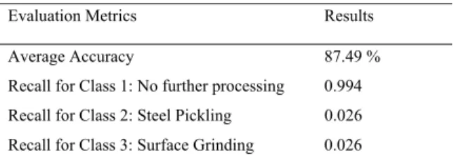
The multivariate time series classification problem for steel quality prediction based on the sensor data is not only complicated due to the irregularities in the input data but also imbalanced structure of the class distribution. In our case almost 85% of the steel slabs had the good quality and no further processing stage was required. The main challenge is identification of the slabs with failures. By applying our multi-stage deep learning classification model directly on the original data, we obtain the average accuracy of 87.49 %. This result can be interpreted positively for relatively balanced datasets (See Table 3). However, a deep look to the recall values of each class reveals that the direct application of the algorithm favors the majority class by getting a recall value 0.994. This value suggests that 99.4% of the steel slabs with good quality were identified by the algorithm. The respective recall values for slabs with surface defects that required steel pickling or surface grinding were 0.026 (for both cases). These results imply that the algorithm could improve the results of the zero (base) model just slightly and was unable to detect the steel products (only 2.6% of them were identified) that require post-processing stages. Despite the obtained high accuracy, the direct application of the model fails to fulfill the requirements of the production managers.
To overcome the problems related to the learning with imbalanced data, a set of diverse (i) data level techniques, (ii) algorithmic level approaches, and (iii) cost-sensitive methods were proposed [26]. The data level methods include randomly oversampling the minority class, randomly undersampling the majority class, informatively oversampling the minority class, informatively undersampling the majority class, and oversampling the small class by generating new synthetic data. The algorithm level approaches investigate the possibilities of adjusting the
248 Mehdiyev, Lahann, Emrich, Enke, Fettke, and Loos / Procedia Computer Science 00 (2017) 000–000 Nijat Mehdiyev et al. / Procedia Computer Science 114 (2017) 242–249
particular algorithm settings to increase the accuracy of classifying the minority class. The third approach, cost-sensitive learning, considers the different penalty costs for misclassifications and forces the model to be able to detect the minority class instances. The scholars suggest that the cost-sensitive learning approaches are better solutions when the costs are unequal for classes [27]. Therefore, in the present paper we adopt the cost-sensitive learning approach. In our multi-class classification problem the costs were simulated by considering diverse decision making and financial settings and transferred to the cost matrix, whose size is defined as the number of classes. In the matrix, the diagonal elements represent the cost of correct classification, with the remaining elements representing the penalty costs for misclassifications [28].
Adopting cost-sensitive learning mechanism lead to a higher recall classifier, but at the same time we flag some fraction of the steel slabs, which had good qualities. Although we end up in the deterioration of the precision and accuracy (from 87.49% to 73.56%), the results obtained from the application of the proposed multi-stage deep learning approach that incorporates the cost preference of the decision makers reveals that the model is now able to detect the both minority classes, steel pickling, and surface grinding. The recall values for these classes were 0.663 and 0.792 respectively, which imply that 66.3% and 79.2% of the steel slabs that required the respective post-processing stages were detected (see Table 4). At the same time, 74.5% of the steel slabs that require no further processing were identified. This results can be considered as satisfactory when including the financial considerations of the decision making process.
Table 3. Direct Classification Table 4. Cost Sensitive Classification
Table 3 and 4 present the results obtained from the deep neural networks classifier with 3 hidden layers, where each layer consist of 200 neurons, by training at 100 epochs and by using ReLU activation function. We have also trained the network by varying the parameters such as changing the activation functions, number of layers and neurons, type of optimization function, and adaptive learning rate. Since no significant deviations from the results were observed for both cases (direct application and cost-sensitive learning), we do not discuss these details explicitly.
6.Conclusion
In the present paper we propose a novel multi-stage deep learning approach for multivariate time series classification problems. After extracting the features from the time series data in an unsupervised manner by using the stacked LSTM Autoencoders, we apply the deep feedforward neural network for making predictions. This approach aims to eliminate the necessity for domain expert knowledge in determination of useful features that are not always available in complex settings. In order to assess the performance of the proposed approach, we use the real world data obtained from a steel industry. The goal of the case study is predicting the post processing activities depending on the detected steel surface defects by using the time series data obtained from the sensors installed in different positions of the continuous steel casting process facility and chemical properties of the steel. Due to the imbalanced nature of the data, we use cost-sensitive learning technique and incorporate the varying preferences of decision makers in making predictions. For the future work, we plan to conduct a comparative analysis of the proposed approach with other types of unsupervised feature learning and classification approaches. We also intend to explore the diverse possibilities to improve the model accuracy by conducting experiments with more data.
Evaluation Metrics Results
Average Accuracy 87.49 %
Recall for Class 1: No further processing 0.994
Recall for Class 2: Steel Pickling 0.026
Recall for Class 3: Surface Grinding 0.026
Evaluation Metrics Results
Average Accuracy 73.56 %
Recall for Class 1: No further processing 0.745
Recall for Class 2: Steel Pickling 0.663
Nijat Mehdiyev et al. / Procedia Computer Science 114 (2017) 242–249 249
Mehdiyev, Lahann, Emrich, Enke, Fettke, and Loos / Procedia Computer Science 00 (2017) 000–000
particular algorithm settings to increase the accuracy of classifying the minority class. The third approach, cost-sensitive learning, considers the different penalty costs for misclassifications and forces the model to be able to detect the minority class instances. The scholars suggest that the cost-sensitive learning approaches are better solutions when the costs are unequal for classes [27]. Therefore, in the present paper we adopt the cost-sensitive learning approach. In our multi-class classification problem the costs were simulated by considering diverse decision making and financial settings and transferred to the cost matrix, whose size is defined as the number of classes. In the matrix, the diagonal elements represent the cost of correct classification, with the remaining elements representing the penalty costs for misclassifications [28].
Adopting cost-sensitive learning mechanism lead to a higher recall classifier, but at the same time we flag some fraction of the steel slabs, which had good qualities. Although we end up in the deterioration of the precision and accuracy (from 87.49% to 73.56%), the results obtained from the application of the proposed multi-stage deep learning approach that incorporates the cost preference of the decision makers reveals that the model is now able to detect the both minority classes, steel pickling, and surface grinding. The recall values for these classes were 0.663 and 0.792 respectively, which imply that 66.3% and 79.2% of the steel slabs that required the respective post-processing stages were detected (see Table 4). At the same time, 74.5% of the steel slabs that require no further processing were identified. This results can be considered as satisfactory when including the financial considerations of the decision making process.
Table 3. Direct Classification Table 4. Cost Sensitive Classification
Table 3 and 4 present the results obtained from the deep neural networks classifier with 3 hidden layers, where each layer consist of 200 neurons, by training at 100 epochs and by using ReLU activation function. We have also trained the network by varying the parameters such as changing the activation functions, number of layers and neurons, type of optimization function, and adaptive learning rate. Since no significant deviations from the results were observed for both cases (direct application and cost-sensitive learning), we do not discuss these details explicitly.
6.Conclusion
In the present paper we propose a novel multi-stage deep learning approach for multivariate time series classification problems. After extracting the features from the time series data in an unsupervised manner by using the stacked LSTM Autoencoders, we apply the deep feedforward neural network for making predictions. This approach aims to eliminate the necessity for domain expert knowledge in determination of useful features that are not always available in complex settings. In order to assess the performance of the proposed approach, we use the real world data obtained from a steel industry. The goal of the case study is predicting the post processing activities depending on the detected steel surface defects by using the time series data obtained from the sensors installed in different positions of the continuous steel casting process facility and chemical properties of the steel. Due to the imbalanced nature of the data, we use cost-sensitive learning technique and incorporate the varying preferences of decision makers in making predictions. For the future work, we plan to conduct a comparative analysis of the proposed approach with other types of unsupervised feature learning and classification approaches. We also intend to explore the diverse possibilities to improve the model accuracy by conducting experiments with more data.
Evaluation Metrics Results
Average Accuracy 87.49 %
Recall for Class 1: No further processing 0.994
Recall for Class 2: Steel Pickling 0.026
Recall for Class 3: Surface Grinding 0.026
Evaluation Metrics Results
Average Accuracy 73.56 %
Recall for Class 1: No further processing 0.745
Recall for Class 2: Steel Pickling 0.663
Recall for Class 3: Surface Grinding 0.792
Mehdiyev, Lahann, Emrich, Enke, Fettke, and Loos / Procedia Computer Science 00 (2017) 000–000
Acknowledgment
This research was funded in part by the German Federal Ministry of Education and Research under grant number 01IS14004A (project iPRODICT) and 01IS12050 (project PRODIGY).
7.References
[1] S. LaValle, E. Lesser, R. Shockley et al., “Big data, analytics and the path from insights to value,” MIT sloan management review,
52(2), 21 (2011).
[2] T. H. Davenport, and J. G. Harris, [Competing on analytics: The new science of winning] Harvard Business Press, (2007).
[3] S. Yin, S. X. Ding, A. Haghani et al., “A comparison study of basic data-driven fault diagnosis and process monitoring methods on the benchmark Tennessee Eastman process,” Journal of Process Control, 22(9), 1567-1581 (2012).
[4] V. Venkatasubramanian, R. Rengaswamy, K. Yin et al., “A review of process fault detection and diagnosis: Part I: Quantitative model-based methods,” Computers & chemical engineering, 27(3), 293-311 (2003).
[5] Q. Yang, and X. Wu, “10 challenging problems in data mining research,” International Journal of Information Technology & Decision Making, 5(04), 597-604 (2006).
[6] G. E. Batista, X. Wang, and E. J. Keogh, "A complexity-invariant distance measure for time series." 699-710.
[7] A. Nanopoulos, R. Alcock, and Y. Manolopoulos, “Feature-based classification of time-series data,” International Journal of Computer Research, 10(3), 49-61 (2001).
[8] T.-c. Fu, “A review on time series data mining,” Engineering Applications of Artificial Intelligence, 24(1), 164-181 (2011).
[9] M. Längkvist, L. Karlsson, and A. Loutfi, “A review of unsupervised feature learning and deep learning for time-series modeling,” Pattern Recognition Letters, 42, 11-24 (2014).
[10] F. C. Morabito, M. Campolo, C. Ieracitano et al., "Deep convolutional neural networks for classification of mild cognitive impaired and Alzheimer's disease patients from scalp EEG recordings." 1-6.
[11] Y. Zheng, Q. Liu, E. Chen et al., "Time series classification using multi-channels deep convolutional neural networks." 298-310. [12] G. E. Hinton, and R. R. Salakhutdinov, “Reducing the dimensionality of data with neural networks,” science, 313(5786), 504-507
(2006).
[13] P. Malhotra, A. Ramakrishnan, G. Anand et al., “Lstm-based encoder-decoder for multi-sensor anomaly detection,” arXiv preprint arXiv:1607.00148, (2016).
[14] K. Cho, B. Van Merriënboer, C. Gulcehre et al., “Learning phrase representations using RNN encoder-decoder for statistical machine translation,” arXiv preprint arXiv:1406.1078, (2014).
[15] J. Li, M.-T. Luong, and D. Jurafsky, “A hierarchical neural autoencoder for paragraphs and documents,” arXiv preprint arXiv:1506.01057, (2015).
[16] S. Bengio, O. Vinyals, N. Jaitly et al., "Scheduled sampling for sequence prediction with recurrent neural networks." 1171-1179. [17] J. Schmidhuber, “Deep learning in neural networks: An overview,” Neural Networks, 61, 85-117 (2015).
[18] X.-W. Chen, and X. Lin, “Big data deep learning: challenges and perspectives,” IEEE Access, 2, 514-525 (2014).
[19] M. A. Nielsen, “Neural networks and deep learning,” URL: http://neuralnetworksanddeeplearning. com/.(visited: 01.11. 2014), (2015).
[20] E. M. Popa, and I. Kiss, “ASSESSMENT OF SURFACE DEFECTS IN THE CONTINUOUSLY CAST STEEL,” Acta Technica
Corviniensis-Bulletin of Engineering, 4(4), 109 (2011).
[21] M. Zaharia, R. S. Xin, P. Wendell et al., “Apache Spark: a unified engine for big data processing,” Communications of the ACM,
59(11), 56-65 (2016). [22] F. Chollet, [Keras], (2015).
[23] D. Team, “Deeplearning4j: Open-source distributed deep learning for the JVM,” Apache Software Foundation License, 2.
[24] M. Hall, E. Frank, G. Holmes et al., “The WEKA data mining software: an update,” ACM SIGKDD explorations newsletter, 11(1), 10-18 (2009).
[25] N. Mehdiyev, D. Enke, P. Fettke et al., “Evaluating Forecasting Methods by Considering Different Accuracy Measures,” Procedia Computer Science, 95, 264-271 (2016).
[26] Y. Sun, A. K. Wong, and M. S. Kamel, “Classification of imbalanced data: A review,” International Journal of Pattern Recognition and Artificial Intelligence, 23(04), 687-719 (2009).
[27] Z.-H. Zhou, and X.-Y. Liu, “Training cost-sensitive neural networks with methods addressing the class imbalance problem,” IEEE Transactions on Knowledge and Data Engineering, 18(1), 63-77 (2006).