A Compact Evolutionary Interval-Valued Fuzzy Rule-Based Classification System for the Modeling and Prediction of Real-World Financial Applications With Imbalanced Data

This work was supported in part by the Spanish Ministry of Science and Technology under Project TIN2011-28488 and Project TIN2013-40765.

J. Sanz and H. Bustince are with the Department of Automática y Computación, Universidad Publica de Navarra, 31006 Pamplona, Spain (+34 948 166 408; fax: +34 948 168 924; e-mail: [email protected]; [email protected]).

D. Bernardo and H. Hagras are with the Computational Intelligence Centre, University of Essex, Wivenhoe Park, Colchester, UK.

F. Herrera is with the Department of Computer Science and Artificial Intelligence, Research Center on Information and Communications Technology (CITIC-UGR), University of Granada, 18071 Granada, Spain and with the Faculty of Computing and Information Technology - North Jeddah, King Abdulaziz University, 21589, Jeddah, Saudi Arabia (e-mail: [email protected]).

Abstract— The current financial crisis has stressed the need of obtaining more accurate prediction models in order to decrease the risk when investing money on economic opportunities. In addition, the transparency of the process followed to make the decisions in financial applications is becoming an important issue. Furthermore, there is a need to handle the real-world imbalanced financial data sets without using sampling techniques which might introduce noise in the used data. In this paper, we present a compact evolutionary interval-valued fuzzy rule-based classification system, which is based on IVTURSFARC-HD(Interval-Valued fuzzy rule-based classification system with TUning and Rule Selection) [22]), for the modeling and prediction of real-world financial applications. This proposed system allows obtaining good predictions accuracies using a small set of short fuzzy rules implying a high degree of interpretability of the generated linguistic model. Furthermore, the proposed system deals with the financial imbalanced datasets with no need for any preprocessing or sampling method and thus avoiding the accidental introduction of noise in the data used in the learning process. The system is also provided with a mechanism to handle examples that are not covered by any fuzzy rule in the generated rule base. To test the quality of our proposal, we will present an experimental study including eleven real-world financial datasets. We will show that the

proposed system outperforms the original C4.5 decision tree, type-1 and interval-valued fuzzy counterparts which use the SMOTE sampling technique to preprocess data and the original FURIA, which is a fuzzy approximative classifier. Furthermore, the proposed method enhances the results achieved by the cost sensitive C4.5 and it gives competitive results when compared with FURIA using SMOTE, while our proposal avoids pre-processing techniques and it provides interpretable models that allow obtaining more accurate results.

Index Terms— Financial applications, Interval-Valued Fuzzy Sets, Interval-Interval-Valued Fuzzy Rule-Based Classification Systems, Evolutionary algorithms.

1.

I

The recent financial crisis highlighted fundamental weaknesses in the long term global approach to financial modeling and prediction. Hence, there is a need for new more comprehensive, transparent and accurate financial modeling and prediction approaches to capitalize on economic opportunities without incurring high levels of unexpected risk.

Many financial applications rely on the expertise of their staff to make a judgment call even when the factors in consideration are too broad and complex to be adequately assessed by the human brain. This

A Compact Evolutionary Interval-Valued Fuzzy

Rule-Based Classification System for the

Modeling and Prediction of Real-World

Financial Applications with Imbalanced Data

might result in the risks being assessed incompletely and inaccurately with a lack of decision consistency. For example, loan officers usually apply the rule of the five C principles (Capacity, Capital, Character, Collateral, and Conditions) to decide whether to grant a loan or not. In order to make accurate and consistent decision with this rule it would be necessary to have complete knowledge of the applicant and there is a need for consistency across the loan officers where each officer should make the same decision for the same applicant, which might not be the case.

In financial applications, as in many real-world problems, the data is highly imbalanced. For example, in a credit card application the number of good customers is much higher than that of bad customers and in fraud detection the majority of the data are normal transactions whereas a few fraudulent transactions are usually present. Most classifiers designed for minimizing the global error rate perform poorly on imbalanced datasets because they misclassify most of the data belonging to the class represented by few examples [1], [2]. To tackle this problem, pre-processing techniques like under-sampling or over-under-sampling are usually applied but both of them present problems. On the one hand, under-sampling techniques may increment the noise since they could eliminate some important patterns. On the other hand, over-sampling techniques, like Synthetic Minority Oversampling Technique (SMOTE) [3], may add noise for the original input data or violate the inherent geometrical structure of the minority and majority classes [4]. Hence, in financial applications it is not desirable to preprocess or sample the data as this could cause big problems.

Real-world financial problems have been tackled using several machine learning and artificial intelligence techniques. The majority of commercial financial systems rely on statistical regression techniques because they provide good results when facing prediction problems composed of two output categories. Other kinds of machine learning techniques applied in financial domains are support vector machines, which were applied to forecast financial time series [5] and to effectively manage governmental funds to small and medium enterprises [6]. Neural networks were applied in a big number of financial applications [7], [8], [9]. However, the drawback of such advanced machine learning techniques is that although they can give good

prediction accuracies, they provide black box models which are very difficult to understand and analyze by a financial analyst. Therefore, they do not fulfil the current common requirements of having an explanation of the reasoning behind a given financial decision.

Trust is the main reason why it is important to provide the end user with easily interpretable models. Regardless of the degree of sophistication of our economies, all transactions still come down to trust. Therefore, transparency is required so that it is possible to know how the given financial models are operating. This need for transparency is reflected in legislations that force financial institutions to disclose the reasoning behind their financial decisions and models.

Decision trees and Fuzzy Rule-Based Systems (FRBSs) are examples of white box transparent models which have been applied for various financial applications ¡Error! No se encuentra el origen de la referencia.. FRBSs have been successfully applied on credit approval, loan portfolio, bankruptcy prediction and security management ¡Error! No se encuentra el origen de la referencia.. The main challenge faced in these works when working with real-world data is the high level of data imbalance. Most of the previous works use preprocessing techniques which might introduce noise and uncertainty.

Interval-Valued Fuzzy Rule-Based Classification Systems (IV-FRBCSs) [19], [20] are interpretable classifiers because they use linguistic terms, which are modeled with Interval-Valued Fuzzy Sets [21] (IVFSs), in the antecedents of the rules. IVTURS FARC-HD [22] (Interval-Valued fuzzy rule-based classification system with TUning and Rule Selection) is a novel IV-FRBCS that provides an accurate as well as a transparent model. The inference process of this system uses interval information in all the steps and it applies Interval-Valued Restricted Equivalence Functions (IV-REFs) [23], [24] to measure the equivalence between the interval membership degrees and the ideal interval membership degrees. Furthermore, IVTURSFARC-HD applies an evolutionary algorithm to modify the values used in the construction of the IV-REFs. This system is designed for standard classification problems, which means that it cannot easily deal with the imbalanced data available in financial applications without preprocessing techniques.

In this paper, we will present a compact evolutionary IV-FRBCS based on IVTURSFARC-HD for the modeling and prediction of financial applications with imbalanced data, with the aim of providing an accurate, comprehensible, transparent and interpretable model. In order to face the usual problems presented in financial domains with imbalanced data and trying to get a small set of short fuzzy rules (interpretable model), we introduce the following techniques:

• A rescaling method to balance the weights of the fuzzy rules associated with the different classes. In this manner, the imbalanced problem is faced internally by the proposed method, which means that sampling/preprocessing techniques are not needed.

• A technique to classify the incoming examples even if they do not match any fuzzy rule in the generated rule base. To do so, the similarity among the uncovered example and the rules is considered.

• An evolutionary process used to perform a rule selection process along with the tuning of both the shape and the lateral position of the IVFSs as well as the values used to construct the IV-REFs. This allows maximizing the classification performance and producing compact and interpretable models.

The quality of our new proposal, which is denoted IVTURSFARC-HD with Rescaling Rule Weight for Imbalanced classification (IVTURSRRW_I ), has been tested thorough various experiments using real-world data sets from eleven financial applications. The obtained results, which are statistically supported, show that IVTURSRRW_I outperforms the original C4.5 method [25] as well as type-1 and interval-valued fuzzy counterparts which used the SMOTE sampling technique to preprocess data. Furthermore, our proposal notably enhances the results achieved by the cost sensitive C4.5 [26] and it gives competitive results versus an approximative fuzzy classifier like FURIA [27] when it uses SMOTE. This fact strengthens the quality of our new method because it provides an accurate and interpretable model learned from the original data. Therefore, IVTURSRRW_I avoids using pre-processing techniques and give accurate results as well as producing a reduction in the number of generated rules, which implies providing more

transparent and highly interpretable models.

This paper is arranged as follows: Section 2 provides some needed background material and the related work about FRBCSs. The proposed compact evolutionary IVTURSRRW_I is presented in Section 3. The experimental results are shown in Section 4 while the conclusions are drawn in Section 5.

2.

B

In this section, we present the background needed to understand the remainder of the paper. We start by presenting some theoretical concepts about IVFSs. Then, we describe the problem of the imbalanced data-sets in classification and finally, we briefly introduce the fuzzy association rules for classification along with the two state-of-the-art fuzzy association rule-based classification models considered in this paper.

2.1Interval-Valued Fuzzy Sets

Fuzzy Sets (FSs) [28] assign crisp values as membership degrees of the elements to the sets whereas IVFSs [21] assign intervals instead of numbers as membership degrees. IVFSs have been successfully applied in various applications including image processing [23], assessment of soil and water conservation [29] and classification [30] among others.

Let us denote by 0, 1 the set of all closed subintervals in 0,1 , that is,

0, 1 = = , |0 ≤ ≤ ≤ 1!. (1) We must remark that we will denote an interval in bold-face and a crisp value in normal-font, that is, is an interval and is a crisp value.

Definition 1 [21,31,32,33] An interval-valued fuzzy set # on the universe $ ≠ ∅ is a mapping

#'(: $ → 0, 1 , such that

#'( +, = # +, , # +, ∈

0, 1 , ./0 122 +, ∈ $. (2)

Obviously, # +_, , # +_, is the interval membership degree of the element +_, to the IVFS #. Our interpretation of the interval membership degree is that the membership degree is a number within the interval but its real value it is not known. The length of the interval membership degree, 3#_'( +_, 4 =

# +, − # +, , can be seen as a representation of the ignorance related to the assignment of crisp values as the membership degrees of the elements to the set. Such ignorance degree can be quantified by means of weak ignorance functions [20].

In order to determine the largest interval membership degree, we need to use a total order relationship for intervals. A method to construct different linear orders between intervals can be found in [34], [35]. A particular case of these linear orders is the one defined by Xu and Yager in [36], which is based on the score and accuracy degrees as shown in Equation (3).

, ≤ 67, 78 if and only A. + < 7 + 7 or + = 7 + 7 and − ≥ 7 − 7 (3)

Using this total order relationship, it is easy to prove that 0, 0 and 1, 1 are the smallest and the largest element of 0, 1 , respectively. So, they are the smallest and the largest interval membership degrees.

In addition, we present the interval operations which will be used to make the computation with intervals both in the inference process and in the computation of the rule weight as an element of

0, 1 instead of with numbers. Let

, , 67, 78 be two intervals, with , , 7, 7 ∈ ℝG, so that , ≤_H 67, 78, which means that ≤ 7 , ≤

7 (this is not a total order relationship for intervals), and 7 > 0 the rules of interval arithmetic are as follows [36]: • Addition: , + 67, 78 = 6 + 7, + 78 (4) • Subtraction: , − 67, 78 = 6J7 − J , K7 − K8 (5) • Product: , ∗ 67, 78 = 6 ∗ 7, ∗ 78 (6) • Division: M,M 6N,N8= O⋀ Q M N, M NR , ⋁ Q M N, M NRT (7)

where ∧ represents the t-norm (minimum) whereas ∨ represents the t-conorm (maximum).

Finally, we recall the definition of IV-REFs [23],[24], which are used to measure the similarity between two intervals. These functions are applied in the inference process of the method used as the base of our new proposal, i.e. IVTURSFARC-HD. We also recall the construction method of these functions that is based on automorphisms, which are continuous

and strictly increasing functions W: 0, 1 → 0, 1 so that W 0 = 0 and W 1 = 1. For example if we use

W = X_{, each value of 1 ∈ 0, ∞ will generate}

an automorphism.

Definition 2 [23], [24] An interval-valued restricted equivalence function associated with an interval-valued negation Z is a function

[\ − ]^_: 0, 1 ` _{→ 0, 1 (8)}

So that:

IR1) [\ − ]^_ , a = [\ − ]^_ a, for all , a ∈ 0, 1 ;

IR2) [\ − ]^_ , a = 1, 1 if and only if

= a;

IR3) [\ − ]^_ , a = 0, 0 if and only if

= 1, 1 and a = 0, 0 or = 0, 0 and

a = 1, 1 ;

IR4) [\ − ]^_ , a = [\ −

]^_ Z , Z a with Z being an involutive interval-valued negation [31], [38];

IR5) For all , a, b ∈ 0, 1 , if

≤H a ≤H b, then [\ −

]^_ , a ≥H [\ − ]^_ , b and [\ −

]^_ a, b ≥H [\ − ]^_ , b .

The construction method of IV-REFs used in this paper, which is based on the construction method of REFs introduced in [39], is the following one: [\ − ]^_ c , , 67, 78d = 6e QWf f_{c1 − JW} `3 4 − W`c7dJd , Wff 1 − |W` − W` 7 | R , g QWffc1 − JW`3 4 − W`c7dJd , Wff 1 − |W` − W` 7 | R8 (9) where W_f = X and W_` = h with 1, i ∈

0.01, 100 , e and g represent a norm and a t-conorm respectively. We must point out that this IV-REF is associated with the interval-valued negation Z , = 6W_{`</sub>f31 − W<sub>`} 4, W_`fc1 −

W`3 4d8.

Example 1 Let 1 = 1 and b = 1, the automorphisms used in Equation 9 are W_f = and W_` = respectively. Let T and S be the minimum and the maximum respectively, Equation 9 can be rewritten as

[\ − ]^_ c , , 67, 78d = 6⋀ c1 − J − 7J , 1 − | − 7|d , ⋁ c1 − J − 7J , 1 − | − 7|d 8 10

with the negation k , = 1 − , 1 − and let = , = 0, 0, a = 67, 78 = 0.3,0.6 and

b = n, n = 1,1 be three intervals, the conditions IR1- IR5 fulfill as shown below

IR1) [\ − ]^_ , a = [\ − ]^_ a, ⇒ 0.4, 0.7 = 0.4, 0.7 IR2) [\ − ]^_ , a = 0.4, 0.7 whereas [\ − ]^_ a, a = 1, 1 IR3) [\ − ]^_ , a = 0.4, 0.7 whereas [\ − ]^_ , b = 0, 0 IR4) [\ − ]^_ , a = [\ − ]^_ Z , Z a ⇒[\ − ]^_ 0,0 , 0.3,0.6 = [\ − ]^_ 1, 1 , 0.4, 0.7 ⇒ 0.4, 0.7 = 0.4, 0.7 IR5) if ≤_Ha ≤_H b, then [\ − ]^_ , a ≥H [\ − ]^_ , b and [\ − ]^_ a, b ≥H[\ − ]^_ , b ⇒ ≤Ha ≤H b, therefore [0.4, 0.7] ≥_H [0, 0] and [0.3, 0.4] ≥_H [0, 0] 2.2Imbalanced Data-Sets in Classification

During the last years, as the popularity of data mining is growing, the machine learning techniques have been applied to several real-world problems, like financial problems. Real-world problems usually contain few examples of the concept to be described due to rarity or the cost to obtain it. The learning from these kinds of problems has been identified as one of the main challenges in data mining [40].

The imbalanced data-sets problem are very common in real world financial data-sets, where one or more classes are represented by a large number of examples (known as majority class) while the other classes are represented by only few examples (known as minority class) [41]. This problem causes the classifier to predict the samples of the majority class and completely ignore the minority ones.

An important aspect when dealing with imbalanced data-sets is the selection of an appropriate metric to measure the performance of the proposals. The most straightforward way to evaluate the performance of classifiers is the analysis based on the confusion matrix. Table 1 shows a confusion matrix for a two-class problem. From this table it is possible to extract a number of widely used metrics to measure the performance of learning systems, such as error rate defined in Equation (11) and accuracy defined in Equation (12) as follows:

^00 = _r + _k / er + _r + ek + _k 11

#tt =_uvGxvGuwGxwuvGuw = 1 − ^00 12

The accuracy is the most commonly used metric for empirical evaluations but for classification in this framework this metric might lead to erroneous conclusions since the minority class has little impact on accuracy compared to the majority class [42]. Therefore, in the framework of imbalanced problems there are more accurate metrics. For instance, from Table 1 four performance measures can be derived in order to take into account the classification rate of each class independently:

• True positive rate (er_zX{|): is the percentage of correctly classified examples belonging to the minority class.

• True negative rate (ek_zX{|): is the percentage of correctly classified examples belonging to the majority class.

• False positive rate (_r_zX{|): is the percentage of misclassified examples belonging to the majority class.

• False negative rate (_k_zX{|): is the percentage of misclassified examples belonging to the minority class.

TABLE 1CONFUSSION MATRIX FOR A TWO-CLASS PROBLEM. MINORITY PREDICTION MAJORITY PREDICTION MINORITY CLASS TRUE POSITIVE (TP) FALSE NEGATIVE (FN) MAJORITY CLASS FALSE POSITIVE (FP) TRUE NEGATIVE (TN)

A well-known metric that attempts to maximize the accuracy of each class is the geometric mean, which is defined as follows [43]:

}~ = •erzX{|∗ ekzX{| 13

2.2.1 Fuzzy Association Rules for Classification This section is aimed at providing a brief introduction of fuzzy association rule-based classifiers, since it is the methodology used by the state-of-the-art fuzzy classification techniques used in this paper, which are FARC-HD [44] and IVTURS [22] that are briefly in Sections 2.3.1 and 2.3.2, respectively.

Association discovery is widely used in data mining since it allows interesting knowledge to be discovered in large databases [45]. Association rules represent dependencies among items in a database using expression like # → €, where # and € are sets of items and # ∩ € ≠ ∅ [46]. The use of fuzzy logic in association rules allows both dealing with uncertain and inaccurate data and introducing linguistic terms implying the generation of an interpretable model for the end users.

The task of classification [47], which aims at determining the class to which the patterns belong, can be tackled using fuzzy association rules. In this case, the antecedent part of the fuzzy rules is composed of fuzzy terms whereas the consequent part has the predicted class label and the rule weight which is written as follows:

]‚: If f is #‚f and … and ƒis #‚ƒ then Class = „‚

with ]…_‚, (14) where ]_‚ is the label of the rule, = _f, … , _ƒ is a n-dimensional example vector, #_‚, is an antecedent fuzzy set representing the variable A in rule ‡, „_‚ is a class label and ]…_‚ ∈ 0, 1 is the rule weight [48]. The fuzzy rule in Equation (14) can be represented as #_‚ → „_‚, where #_‚ = 3#_‚f, … , #_‚ƒ4.

Let _ˆ= 3 _ˆf, … , _ˆƒ, 4, ‰ = 1, 2, … , k be a set of k labeled examples from ~ classes of an Š -dimensional classification problem. The matching degree of each training example _ˆ with the antecedent #_‹ is defined as follows:

Œ•Ž3 ˆ4 = e QŒ•Ž•3 ˆf4, … , Œ•Ž•3 ˆƒ4R, 15 where Œ_•Ž’ ∙ is the membership function of the antecedent fuzzy set #_‚, and e is a t-norm.

The support of the fuzzy rule #_‚ → „_‚ , which can be viewed as the coverage of the training examples by the fuzzy rule, is written as follows

g+‰‰/0”3#‚→ „‚4 =

∑_{™˜∈š›œ•• šŽ}–_—Ž3M˜4

|w| 16

The confidence of the fuzzy rule #_‚ → „_‚ , which can be viewed as the validity of the fuzzy rule, is written as follows

„/Š.AžŸŠtŸ3#‚ → „‚4 =

∑M_{˜∈š›œ•• šŽ}Œ•Ž3 ˆ4

∑wˆ fŒ•_Ž3 ˆ4 17

2.2.2 Fuzzy Association Rules for Classification for High Dimensional Problems

In [44], Alcalá-Fdez et al. defined the algorithm known as FARC-HD (Fuzzy Association Rule-based Classification model for High Dimensional problems). This method allowed outperforming the performance provided by ten well-known classifiers. Furthermore, it generates a compact set of rules with a small computational effort. This fuzzy classifier is composed of the following three stages:

1. Fuzzy association rule extraction for classification. In this step the rule base is generated. To do so, a search tree is generated for each class in which the frequent itemsets are computed by applying the support (see Equation (16)) and the confidence (see Equation (17)). In this method each item is represented by a fuzzy term and the depth of the tree is limited by a predefined parameter. Once the search tree is completed, a fuzzy association classification rule is generated for each frequent itemset. To do so, the path of the frequent itemset is assigned as the antecedent part, the class of the search tree is set as class label and the confidence is assigned as rule weight.

2. Candidate rule prescreening. In this step a pattern weighting scheme is carried out to select the most promising set of rules for each class, since in the first stage a huge number of fuzzy rules can be generated. To do so, each pattern has assigned a weight that is meant to be the strength in which it contributes in the computation of the quality of the rules. The improved weighted relative accuracy measure [44] is applied to compute the quality of the rules. An iterative process is carried out in which in each run the best rule is selected and the weights of the patterns are decreased based on the covering of such rule. This process is repeated until a stopping criterion is fulfilled.

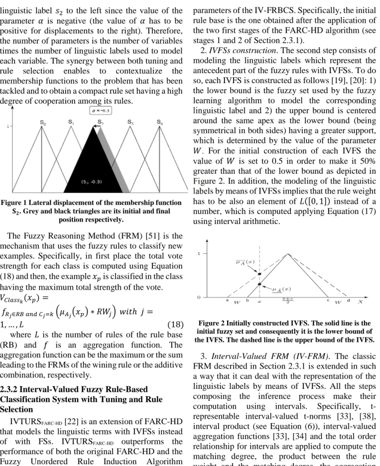
3. Rule selection and lateral tuning. The final stage of the method consists of selecting and tuning a set of rules starting from the final rule base obtained in the second stage. To this aim, the tuning of the lateral position of the linguistic labels [49], which is based on the linguistic 2-tuples representation [50], combined with a genetic rule selection process is applied. For the lateral tuning the parameter ¡, which determines the position of the linguistic labels, is tuned for each linguistic label of the system. Figure 1 shows an example of the lateral displacement of the

linguistic label ¢_` to the left since the value of the parameter ¡ is negative (the value of ¡ has to be positive for displacements to the right). Therefore, the number of parameters is the number of variables times the number of linguistic labels used to model each variable. The synergy between both tuning and rule selection enables to contextualize the membership functions to the problem that has been tackled and to obtain a compact rule set having a high degree of cooperation among its rules.

Figure 1 Lateral displacement of the membership function £¤. Grey and black triangles are its initial and final

position respectively.

The Fuzzy Reasoning Method (FRM) [51] is the mechanism that uses the fuzzy rules to classify new examples. Specifically, in first place the total vote strength for each class is computed using Equation (18) and then, the example _ˆ is classified in the class having the maximum total strength of the vote.

\¥¦X§§_¨ ˆ =

.©Ž∈©ª Xƒ« ¥Ž ¬cŒ•Ž3 ˆ4 ∗ ]…‚d -A”® ‡ =

1, … , 18 where is the number of rules of the rule base (RB) and . is an aggregation function. The aggregation function can be the maximum or the sum leading to the FRMs of the wining rule or the additive combination, respectively.

2.3.2 Interval-Valued Fuzzy Rule-Based Classification System with Tuning and Rule Selection

IVTURSFARC-HD [22] is an extension of FARC-HD that models the linguistic terms with IVFSs instead of with FSs. IVTURSFARC-HD outperforms the performance of both the original FARC-HD and the Fuzzy Unordered Rule Induction Algorithm (FURIA) [27]. This method is composed of the following steps:

1. Rule base generation. This method learns an initial type-1 FRBCS so as to initialize the

parameters of the IV-FRBCS. Specifically, the initial rule base is the one obtained after the application of the two first stages of the FARC-HD algorithm (see stages 1 and 2 of Section 2.3.1).

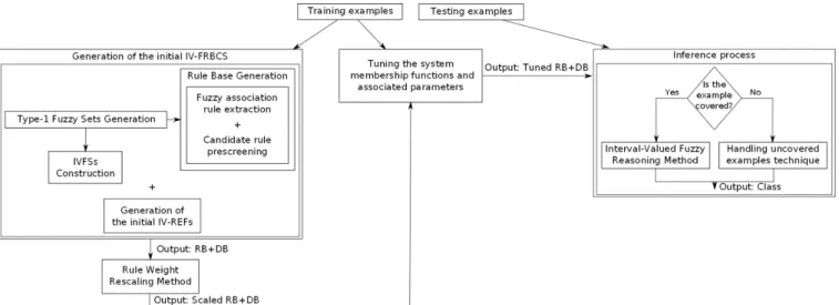
2. IVFSs construction. The second step consists of modeling the linguistic labels which represent the antecedent part of the fuzzy rules with IVFSs. To do so, each IVFS is constructed as follows [19], [20]: 1) the lower bound is the fuzzy set used by the fuzzy learning algorithm to model the corresponding linguistic label and 2) the upper bound is centered around the same apex as the lower bound (being symmetrical in both sides) having a greater support, which is determined by the value of the parameter

…. For the initial construction of each IVFS the value of … is set to 0.5 in order to make it 50% greater than that of the lower bound as depicted in Figure 2. In addition, the modeling of the linguistic labels by means of IVFSs implies that the rule weight has to be also an element of 0, 1 instead of a number, which is computed applying Equation (17) using interval arithmetic.

Figure 2 Initially constructed IVFS. The solid line is the initial fuzzy set and consequently it is the lower bound of the IVFS. The dashed line is the upper bound of the IVFS.

3. Interval-Valued FRM (IV-FRM). The classic FRM described in Section 2.3.1 is extended in such a way that it can deal with the representation of the linguistic labels by means of IVFSs. All the steps composing the inference process make their computation using intervals. Specifically, t-representable interval-valued t-norms [33], [38], interval product (see Equation (6)), interval-valued aggregation functions [33], [34] and the total order relationship for intervals are applied to compute the matching degree, the product between the rule weight and the matching degree, the aggregation function . and the final prediction, respectively. Furthermore, the idea of the maximum similarity classifier is introduced in the computation of the

matching degree. To do so, IV-REFs are applied to compute the equivalence between the interval membership degrees and the ideal membership degree, 1, 1 , for each attribute of the problem. For the construction of each IV-REF it is necessary to set the value of the parameters 1 and i in Equation (9), which means that their results may vary depending on these values.

4. Rule selection and genetic tuning. The last step is an optimization stage, where a combination of a rule selection process and a tuning approach, as in the previously explained FARC-HD method, is carried out. However, this method does not tune the lateral position of the linguistic labels but the values of the parameters 1 and i used to construct the IV-REF associated with each variable of the problem. Therefore, the number of parameters to be tuned is two times the number of attributes of the problem [22].

3.

T

P

C

E

I

-V

F

R

-B

C

S

F

A

M

P

In this section we present IVTURSRRW_I , which is an IV-FRBCS built on the basis of IVTURSFARC-HD [22], for the modeling and prediction of financial applications which are characterized by highly imbalanced data. The proposed system will handle the imbalanced data (with no need for data pre-processing or sampling) and it is aimed to do the modeling and prediction based on a small set of short

rules which will help to increase the transparency and interpretability of the generated model to the user.

Figure 3 shows an overview of the proposed method, which shares two basic components of the IVTURSFARC-HD method, namely the generation of the initial IV-FRBCS (applying the two first steps introduced in Section 2.3.2) and the IV-FRM. Our new method generates an initial IV-FRBCS using the training examples and then, the created rule base is scaled using the process introduced in Section 3.1. After this steps, it is applied an evolutionary process to adapt the system’s parameters to the problem (using the training examples again), which is described in Section 3.3. When new patterns arrive (testing examples) the method uses the tuned model to classify them: if the example is covered by any fuzzy rule the usual IV-RFM is applied; otherwise, the method defined in Section 3.2 to handle uncovered examples is used.

The novelty of our new method consists of a method to rescale the rule weights of the generated rule base in order to face the imbalance problem at algorithmic level. The rescaling is necessary because when dealing with imbalanced classification problems it is common that the confidence of the minority class rules is low. This fact implies that at classification time most of the examples are classified in the majority class leading to a lack of accuracy in the minority class, which might be the class of interest in financial applications. Additionally, we provide the IV-FRM with a technique that allows one to provide a classification for those examples not matching any rule in the generated rule base. Finally, we propose to use an

evolutionary algorithm to tune the values of the system’ parameters in order to increase its performance as much as possible. Specifically, we tune the parameters defining the IVFSs, namely the lateral position using the parameter α as shown in Figure 1 and the amplitude of the support of the upper bound using the parameter … as shown in Figure 2, as well as the parameters 1 and i used to construct the IV-REFs (see Equation (9)) applied in the computation of the matching degree of the examples with the antecedent of the rules.

In the remainder of this section we describe in detail the three novel techniques, namely the rule weight rescaling method, the mechanism to handle uncovered examples and the tuning proposal.

3.1Rule Weight Rescaling Method

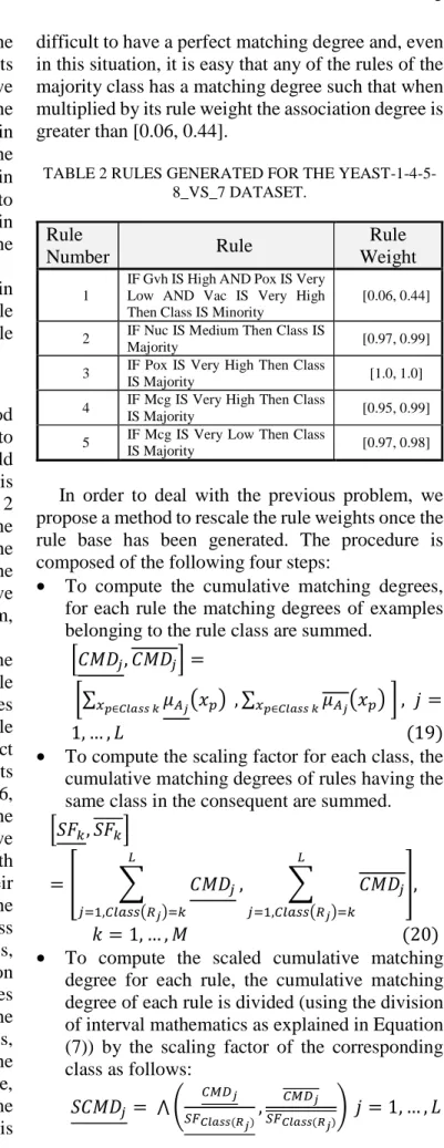
This section is aimed at describing the method used to rescale the rule weight of the rules in order to handle the imbalanced data-sets faced in real world financial applications. The need for this procedure is easily shown in the following example in Table 2 which shows the rule base generated by the IVTURSFARC-HD method for the fourth partition of the Yeast-1-4-5-8_vs_7 dataset (obtained from the KEEL repository [52]). Five linguistic labels have been used for each variable: very low, low, medium, high and very high.

From Table 2 it is observed that there is only one rule belonging to the minority class and its rule weight is small whereas the rule weights of the rules belonging to the majority class are large. If the rule belonging to the minority class had a perfect matching degree ([1, 1] = [1, 1]* [1, 1]* [1, 1]), its association degree would be its rule weight ([0.06, 0.44] = [1, 1]*[0.06, 0.44]). In order to compute the classification soundness degree for each class we aggregate the association degrees (for instance with the maximum) of the rules having that class in their consequents. Following the previous example, the classification soundness degree for the minority class would be [0.06, 0.44]. Regarding the majority class, we have to apply the maximum of the association degrees of rules 2-5. If any of the association degrees of these four rules were greater than [0.06, 0.44] the example would be classified in the majority class, since the predicted class is the one having the greatest classification soundness degree. Therefore, the conditions necessary to classify an example in the minority class are difficult to be fulfilled, since it is

difficult to have a perfect matching degree and, even in this situation, it is easy that any of the rules of the majority class has a matching degree such that when multiplied by its rule weight the association degree is greater than [0.06, 0.44].

TABLE 2 RULES GENERATED FOR THE YEAST-1-4-5-8_VS_7 DATASET.

In order to deal with the previous problem, we propose a method to rescale the rule weights once the rule base has been generated. The procedure is composed of the following four steps:

• To compute the cumulative matching degrees, for each rule the matching degrees of examples belonging to the rule class are summed.

6„~±‚, „~±‚8 =

O∑M˜∈š›œ•• ¨Œ•Ž3 ˆ4 , ∑M˜∈š›œ•• ¨Œ•Ž3 ˆ4 T , ‡ =

1, … , 19 • To compute the scaling factor for each class, the

cumulative matching degrees of rules having the same class in the consequent are summed.

6g_¬, g_¬8 = ³ ´ „~±‚ H ‚ f,¥¦X§§3©Ž4 ¬ , ´ „~±‚ H ‚ f,¥¦X§§3©Ž4 ¬ µ, ¶ = 1, … , ~ 20 • To compute the scaled cumulative matching degree for each rule, the cumulative matching degree of each rule is divided (using the division of interval mathematics as explained in Equation (7)) by the scaling factor of the corresponding class as follows: g„~±‚ = ⋀ · ¥¸¹Ž ºx_{š›œ•• »Ž} , ¥¸¹Ž ºx_{š›œ•• »Ž} ¼ ‡ = 1, … , Rule Number Rule Rule Weight 1

IF Gvh IS High AND Pox IS Very Low AND Vac IS Very High Then Class IS Minority

[0.06, 0.44]

2 IF Nuc IS Medium Then Class IS

Majority [0.97, 0.99]

3 IF Pox IS Very High Then Class

IS Majority [1.0, 1.0]

4 IF Mcg IS Very High Then Class

IS Majority [0.95, 0.99]

5 IF Mcg IS Very Low Then Class

21 g„~±‚ = ⋁ · ¥¸¹_Ž ºx_{š›œ•• »Ž} , ¥¸¹Ž ºx_{š›œ•• »Ž} ¼ ‡ = 1, … , 22 • To compute the scaled support and confidence of

each rule, Equations (16) and (17) are applied using the results computed in the previous step (following the division of interval mathematics as explained in Equation (7)) to result in the scaled support and confidence values:

6g+‰‰/0”º½X¦|«3# → „‚4, g+‰‰/0”º½X¦|«3# → „‚48 = ¾g„~±_{k ,}‚ g„~±_{k ¿ 23}‚ „/Š.AžŸŠtŸº½X¦|«3# → „‚4 = À Á_∑ g„~±_g„~±‚ ¬ ¸ ¬ f , g„~±‚ ∑¸¬ fg„~±¬Â 24 „/Š.AžŸŠtŸº½X¦|«3# → „‚4 = à Á_∑ g„~±_g„~±‚ ¬ ¸ ¬ f , g„~±‚ ∑¸¬ fg„~±¬Â 25

• To compute the rule weight, the scaled support and confidence of each rule are multiplied (using the multiplication of interval mathematics as explained in Equation (6)) and assigned as the rule weight. ]…‚= g+‰‰/0”º½X¦|«3# → „‚4 ∗ „/Š.AžŸŠtŸº½X¦|«3# → „‚4, ‡ = 1, … , 26 ]…‚= g+‰‰/0”º½X¦|«3# → „‚4 ∗ „/Š.AžŸŠtŸº½X¦|«3# → „‚4, ‡ = 1, … , 27

3.2Handling Inputs Not Matching Rules in

the Rule Base

The rule learning method used by FARC-HD is able to create rules whose maximum number of antecedents can be programmatically limited using the maximum tree depth. Therefore, it creates a compact rule base composed of short rules, which helps increasing both the interpretability and the readability of the model and it also implies a

reduction of the computational time needed to classify an example.

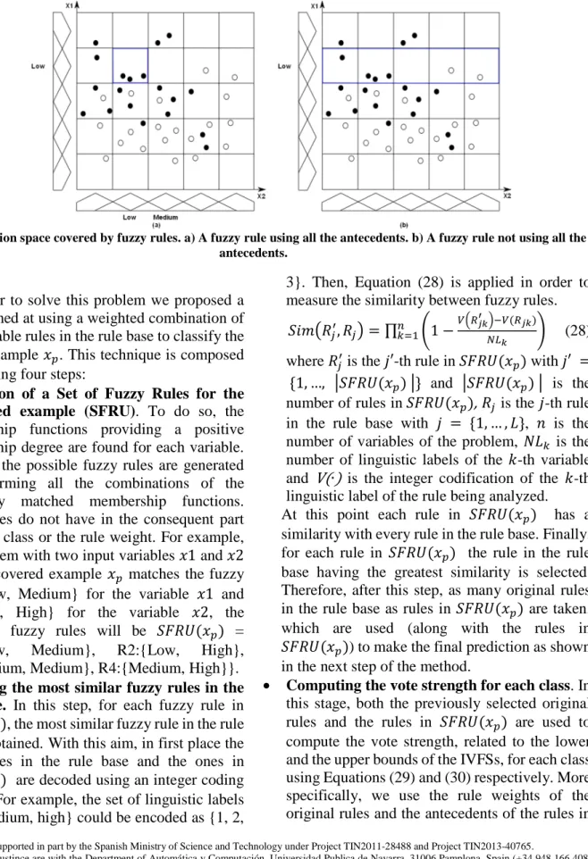
According to the fuzzy rule learning algorithm used by the FARC-HD method, if we set the maximum tree depth to the number of variables of the problem, a rule base composed of fuzzy rules whose antecedent length is equal to the number of variables could be generated. In this situation, the created fuzzy rules would cover very narrow areas of the solution space, which could provoke an increase on the system’s accuracy at the expense of a reduction of the system’s interpretability since both the rule length and the number of generated fuzzy rules would be greater. Figure 4a depicts a specific fuzzy rule (IF _f is Low and _` is Low) covering a narrow area whereas a generic fuzzy rule (IF _f is Low) is shown in Figure 4b. Although FARC-HD could generate both types of rules, it usually creates generic fuzzy rules like the later one.

A big problem encountered when producing specific rules is that some regions of the solution space could not be covered by any fuzzy rule. This situation happens in those cells shown in Figure 4a where there are no examples (like the cell {Low, Medium}), since specific rules (like Rule: {Low, Low}) are generated for cells having examples. This situation provokes the need of providing the system with a mechanism to classify examples that are not covered by any fuzzy rule in the rule base. There are two main approaches to handle this situation: 1) to reject the input without providing a prediction for the example and hence the example is not considered to compute the er_zX{| and ek_zX{|; 2) to build a default rule that always classifies uncovered examples in the majority class.

The first approach is unacceptable solution for the financial domain where the prediction system should always be able to provide a prediction. The second approach avoids the problem of not providing a prediction but if the prediction capability over the uncovered examples is measured applying the geometric mean the achieved result will be always 0. This is due to the fact that the default rule correctly classifies all the examples of the majority class (ek_zX{|=1) whereas it misclassifies all the examples of the minority class (er_zX{|= 0).

This work was supported in part by the Spanish Ministry of Science and Technology under Project TIN2011-28488 and Project TIN2013-40765.

J. Sanz and H. Bustince are with the Department of Automática y Computación, Universidad Publica de Navarra, 31006 Pamplona, Spain (+34 948 166 408; fax: +34 948 168 924; e-mail: [email protected]; [email protected]).

D. Bernardo and H. Hagras are with the Computational Intelligence Centre, University of Essex, Wivenhoe Park, Colchester, UK.

F. Herrera is with the Department of Computer Science and Artificial Intelligence, Research Center on Information and Communications Technology (CITIC-UGR), University of Granada, 18071 Granada, Spain and with the Faculty of Computing and Information Technology - North Jeddah, King Abdulaziz University, 21589, Jeddah, Saudi Arabia (e-mail: [email protected]).

Figure 4 Solution space covered by fuzzy rules. a) A fuzzy rule using all the antecedents. b) A fuzzy rule not using all the antecedents.

In order to solve this problem we proposed a technique aimed at using a weighted combination of the most suitable rules in the rule base to classify the uncovered example _ˆ. This technique is composed of the following four steps:

• Generation of a Set of Fuzzy Rules for the Uncovered example (SFRU). To do so, the membership functions providing a positive membership degree are found for each variable. Then, all the possible fuzzy rules are generated by performing all the combinations of the previously matched membership functions. These rules do not have in the consequent part either the class or the rule weight. For example, in a problem with two input variables 1 and 2 if the uncovered example _ˆ matches the fuzzy sets {Low, Medium} for the variable 1 and {Medium, High} for the variable 2, the generated fuzzy rules will be g_]$ _ˆ = {R1:{Low, Medium}, R2:{Low, High}, R3:{Medium, Medium}, R4:{Medium, High}}.

• Obtaining the most similar fuzzy rules in the

rule base. In this step, for each fuzzy rule in

g_]$ ˆ , the most similar fuzzy rule in the rule base is obtained. With this aim, in first place the fuzzy rules in the rule base and the ones in

g_]$ ˆ are decoded using an integer coding scheme. For example, the set of linguistic labels {low, medium, high} could be encoded as {1, 2,

3}. Then, Equation (28) is applied in order to measure the similarity between fuzzy rules.

gAÄ3]‚Å, ]‚4 = ∏ ·1 −(c©Ž¨

Ç _{d ( ©Ž¨}

wH¨ ¼

ƒ

¬ f (28)

where ]_‚Å is the ‡′-th rule in g_]$ _ˆ with‡′ =

É1, …, Kg_]$ ˆ KÊ and Kg_]$ _ˆ K is the number of rules in g_]$ _ˆ ,]_‚ is the ‡-th rule in the rule base with ‡ = É1, … , Ê, Š is the number of variables of the problem, k _¬ is the number of linguistic labels of the ¶-th variable and V ∙ is the integer codification of the ¶-th linguistic label of the rule being analyzed. At this point each rule in g_]$ _ˆ has a similarity with every rule in the rule base. Finally, for each rule in g_]$ _ˆ the rule in the rule base having the greatest similarity is selected. Therefore, after this step, as many original rules in the rule base as rules in g_]$ _ˆ are taken, which are used (along with the rules in

g_]$ ˆ ) to make the final prediction as shown

in the next step of the method.

• Computing the vote strength for each class. In this stage, both the previously selected original rules and the rules in g_]$ _ˆ are used to compute the vote strength, related to the lower and the upper bounds of the IVFSs, for each class using Equations (29) and (30) respectively. More specifically, we use the rule weights of the original rules and the antecedents of the rules in

g_]$ ˆ . \/”ŸË3 ˆ4 = ∑KÍÎ»Ï ™˜ K –_—ŽÇ3M˜4∗©ÌŽÇ ŽÇЕ,š›œ••c»ŽÇdÐÑ ⋁KÍÎ»Ï ™˜ K_{š›œ•• ŽÇ ÐÑ}–_—ŽÇ3M˜4∗©ÌŽÇ (29) \/”ŸË3 ˆ4 = ∑KÍÎ»Ï ™˜ K –_—ŽÇ3M˜4∗©ÌŽÇ ŽÇЕ,š›œ••c»ŽÇdÐÑ ⋁KÍÎ»Ï ™˜ K –_—ŽÇ3M˜4∗©ÌŽÇ š›œ••c»ŽÇdÐÑ (30)

where Œ_•ŽÇ3 _ˆ4 and Œ_‚Å3 _ˆ4 are the lower and upper matching degrees of the example _ˆ with the ‡′-th rule in g_]$ _ˆ whereas ]…_‚Å and

]…‚Å are the lower and upper rule weights of the

most similar rule in the rule base to the ‡′-th rule in g_]$ _ˆ .

• Final prediction of the class. The uncovered example _ˆ will be classified in the class having largest vote strength according to Equation (31).

_ Òf, … , Ò¸

= 10Ó Ä1_{Ë f,…,¸}·\/”ŸË3 ˆ4 + \/”Ÿ₂ Ë3 ˆ4¼ 31

3.3Tuning the System Membership

Functions and the Associated Parameters The last stage of the methodology consists of optimizing the values of the system’s parameters. In this paper we propose to tune both the values determining both the shape and position of the IVFSs and the values of the parameters used to generate the IV-REF associated with each variable of the problem. In this manner, we combine the good features of two common tuning approaches [53], [54], namely the genetic tuning of the knowledge base parameters and the genetic adaptive inference system. Additionally, we perform simultaneously a rule selection process to decrease the system’s complexity.

We use the CHC evolutionary model [55], which is short for Cross generational elitist selection, Heterogeneous recombination and Cataclysmic mutation, to carry out the optimization process, since it is the same method used in the two state-of-the-art fuzzy classifiers used in this paper and it is a good choice in problems having a complex search space. The specific components of our new proposal are: • Coding scheme: The chromosomes use a double

coding scheme. On the one hand, real codification is considered for the tuning

proposals and binary codification is used for the rule selection process. Equation (32) shows the structure of the whole chromosome.

„uÔ{X¦ = É„H, „Ì, „Õ, „©Ê (32) It can be observed that the chromosome is

composed of four parts: the three first parts perform the tuning of the membership functions and the associated parameters and the last part carries out a rule selection process. These parts are described in detail below:

1. Tuning of the lateral position of the linguistic labels (depicted in Figure 2).

„H = ¡ff, … , ¡f¦•, … , ¡ƒf, … , ¡ƒ¦•!, (33) where ¡_,§∈ −0.5, 0.5 , with A = 1, … , Š,¢ =

1, … , 2, and 2_, represents the number of linguistic labels used in the A-th variable.

2. Amplitude of the support of the upper bound of the IVFSs.

„Ì = …ff, … , …f¦•, … , …ƒf, … , …ƒ¦•!, (34) where …_,§ ∈ 0, 1, with A = 1, … , Š, ¢ =

1, … , 2, and 2_, represents the number of linguistic labels used in the A-th variable.

3. Tuning of the equivalence: genes take values in the range [0.01, 1.99]

„Õ = É1f, if, … , 1ƒ, iƒÊ, (35)

where 1_,, i_, ∈ 0.01, 1.99 , with A = 1, … , Š. 4. Rule selection: this part is composed of as

many genes as the number of rules in the rule base. A binary codification is used; therefore the possible values for the genes are 0 or 1, where the values 1 and 0 mean that the associated rule is used or not in the inference respectively.

„© = É]f, … , ]HÊ (36)

where ]_‚ ∈ É0, 1Ê, with ‡ = 1, … , .

• Initialization of the population: we initialize a chromosome representing the initial system, which is the chromosome that encodes the initial set-up of the IV-FRBCS. To do so, we set all the genes performing the lateral tuning to 0.0 (so that the membership functions do not have any lateral displacement), all the genes used to modify the amplitude of the support of the IVFSs are set to 0.5 (in order to make the amplitude of the upper bound 50% greater than that of the lower bound), the ones to carry out the tuning of the equivalence are set to 1.0 (with this setting the identity function is computed) and the genes used to make the rule selection process are set to 1 (to consider

all the rules in the rule base). The remainder individuals are randomly initialized within the ranges demanded in each part.

• Chromosome evaluation: we take the average mean between the accuracy achieved in both classes, which is the area under the ROC curve [56] considering a single point

_A”ŠŸ¢¢ = uvÖœ×ØGuwÖœ×Ø

` (37

We must point out that this fitness function provides a similar behavior to that of the geometric mean, since both of them take into account the accuracy obtained in each class of the problem. In this manner we approximate the results of the geometric mean using a less computational demanding metric.

• Crossover operator: for the part of the chromosome using a real codification we apply the Parent Centrix BLX operator [57] whereas the half uniform crossover [58] is used for the part using the binary codification.

• Restarting approach: the population is randomly initialized and the best individual found so far is included in the population as in the elitist scheme. In this manner, we get away from local optima.

4.

E

R

In this section, we present the experiments and results to validate our proposed system, which is denoted IVTURSRRW_I , for financial applications. The experimental framework used to show the quality of the new method is described in Section 4.1. The study has a double aim, on the one hand, the suitability of the novelties introduced in

IVTURSRRW_I _{needs to be justified (Section 4.2)} and, on the other hand, the benefits of our new method against the use of SMOTE, which is a widely used pre-processing technique, and the cost sensitive C4.5 decision tree are analyzed (Section 4.3). In both scenarios, we present the evaluations carried over eleven different financial applications.

4.1Experimental Framework

In this section we present the framework we have used to test the quality of our new approach. Specifically, we first describe the financial datasets used in the study. Next, we introduce the notation and configuration of the different classifiers and finally, the statistical tests used to validate our results

are presented.

4.1.1 Financial datasets description

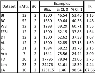
We have used eleven real-world datasets from various financial domains. The features of these datasets are summarized in Table 3, where we can see the names of the datasets, their total number of attributes (#Attr.), classes (#Cl.) and examples (data instances) (#Ex.). We also show the class distribution of the examples according to the classes (% Cl. 0 (% of Class 0) and % Cl. 1(% Class 1)) and the Imbalanced Ratio (IR) [59] of each dataset, which is defined as the ratio of the number of instances of the minority class and the majority class. These datasets and the tables, in which the obtained results are shown, are sorted incrementally according to the IR. TABLE 3 FEATURES OF THE FINANCIAL DATA-SETS

USED IN THE EXPERIMENTAL STUDY.

#Ex. % Cl. 0 % Cl. 1 BI 12 2 1300 46.54 53.46 1.15 BC 52 2 1650 59.64 40.36 1.48 WSI 12 2 1298 39.29 60.71 1.55 FESI 12 2 1300 62.15 37.85 1.64 DT 12 2 1300 62.62 37.38 1.67 AL 12 2 1300 62.85 37.15 1.69 SL 21 2 1894 68.22 31.78 2.15 Arb 7 2 1641 75.56 24.44 3.09 FD 20 2 17795 78.94 21.06 3.75 Len 23 2 24476 81.61 18.39 4.44 LA 10 2 123115 1.46 98.54 67.66 Examples Dataset #Attr. #Cl. IR

The description of each financial dataset is as follows:

• Bank Investment (BI) Data set: is used to predict whether to invest or not by buying or not buying a bank share in stock market. • Bank Credit (BC) Data Set: is a bank credit

card approval application system which is in use by a real-world bank to identify good and bad customers where good customers are non-defaulting customers and bad customers are defaulting customers.

• Western Stock Index (WSI) Data Set: is used for predicting a major Western stock market composite index of whether the stock market index will increase/remain the same or decrease.

• Far Eastern Stock Index (FESI) Data Set: is used for predicting a far eastern stock market composite index of whether the stock market index will increase or remain the same or decrease.

• Digital TV (DT) Data Set: is used for predicting whether to invest or no by buying or not buying a digital TV network share in stock market.

• Airline (AL) Data Set: is applied for predicting whether to invest or no by buying or not buying an airline share in stock market. • Small Loans (SL) Data Set: is used for the evaluation of customers (good or bad customer) for personal small loans applications where there is no knowledge of the customer full credit history.

• Arbitrage (Arb) Data Set: is used for spotting arbitrage opportunities in the London International Financial Futures Exchange (LIFFE) market [10-12]. The data reported in this paper was developed in [12] to identify arbitrage situations by analyzing option and futures prices in the LIFFE market.

• Fraud Detection (FD) Data Set: is used for fraud detection in personal loan application for small loan amounts.

• Lending (Len) Data Set: is used for

evaluation of customers (good or bad customer) for personal small loans applications where there is knowledge of the customer full credit history.

• Loan Authorisation (LA) Data Set: is

related to the prediction of good (profitable) or bad (non-profitable) customers for loan authorization.

In order to carry out the experimental study we have split the data using a random stratified scheme, where 70% of the examples are used to train the system and the remaining 30% of the examples are used to test the generated model.

4.1.2 The Used Configurations and

Notations

In this paper, we compare our proposed compact

evolutionary IV-FRBCS that we call

ÙÚÛÜÝ£_{ÞßÝà áâ}ÝÝã_Ù _{, which is highlighted in grey in} Table 4, with the following algorithms:

• IVTURSFARC-HD: it is a version of our new proposal that do not use the rule weight rescaling method. It will be used to determine the benefits of using the rule weight rescaling method.

• FARC-HD method [44] (FARCHD): it is a state-of-the-art type-1 fuzzy classifier. It will be used to show the suitability of the use of IVFSs.

• IVTURS_FS: it is the type-1 fuzzy counterpart of IVTURSFARC-HD. It also will be considered to analyze the goodness of the use of IVFSs.

• C4.5 [25]: it is the classical C4.5 decision tree. It is included in the study since it is a widely used interpretable method when dealing with classification problems.

• C4.5_CS [26]: it is the C4.5 decision tree modified so that it uses a cost sensitive method to deal with the imbalanced problem at algorithmic level.

• FURIA [27]: it is a state-of-the art type-1 fuzzy approximative classifier.

• SMOTE [3]: it is one of the most used pre-processing techniques. It will be used to check whether the use of IVTURSRRW_I is competitive versus a state-of-the-art pre-processing technique.

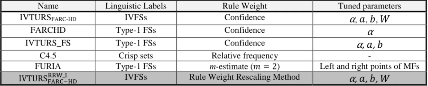
We have to point out that all the classifiers used in the comparison provide an interpretable and transparent model in order to ease the understating of the system by financial analysts. The exception is FURIA, since its linguistic terms are not defined in the same way in the different rules. The notations and descriptions of the features of the classifiers used in the study are shown in Table 4, where the first column shows the name given for each approach, the second one describes the kind of set used to model the linguistic labels, the third column shows the method used to compute the rule weight and the last column specifies the parameters which are tuned in the optimization process.

TABLE 4 NOTATIONS AND DESCRIPTIONS OF THE FIVE APPROACHES. Name Linguistic Labels Rule Weight Tuned parameters

IVTURSFARC-HD IVFSs Confidence α_, 1_, i_, …

FARCHD Type-1 FSs Confidence α

IVTURS_FS Type-1 FSs Confidence α, 1, i

C4.5 Crisp sets Relative frequency -

FURIA Type-1 FSs m-estimate (Ä = 2) Left and right points of MFs

IVTURS ä_å IVFSs Rule Weight Rescaling Method α, 1, i, … In order to conduct a fair comparison, we have

considered the same configurations for the methods based on the FARC-HD algorithm (they can use either type-1 FSs or IVFSs): we have used five linguistic labels (using triangular shaped membership functions) per variable, the interval product (or product when using type-1 FSs) to model the conjunction operator (t-norm) and the FRM of the wining rule (the maximum as aggregation function). The thresholds used in the a-priori algorithm are introduced in Table 5. For the genetic tuning we have considered the following values for their parameters:

• Population size: 50 individuals. • Number of evaluations: 20,000.

• Bits per gene for the Gray codification (for incest prevention): 30.

Regarding the C4.5 decision tree we have used 0.25 and 2 as confidence level and minimum number of examples per leaf, respectively. Finally, we have set the configuration of FURIA as recommended by the authors, that is, three folds and two optimizations.

TABLE 5 CONFIGURATION OF THE FARC-HD METHOD.

Parameter Value

Minimum support 0.01

Minimum confidence 0.9

Maximum tree depth 3

¶{: number of covered times 2

4.1.3 Statistical tests

We will use hypothesis validation techniques in order to give statistical support to the analysis of the presented results [60], [61]. We use non-parametric tests because the initial conditions that guarantee the reliability of the parametric tests cannot be fulfilled, which implies that the statistical analysis loses credibility with these parametric tests [60].

Specifically, we use the Friedman aligned ranks test [62] to detect statistical differences among a group of results and the Holm post-hoc test [63] to find the algorithms that reject the equality hypothesis

with respect to a selected control method.

The post-hoc procedure allows us to know whether a hypothesis of comparison could be rejected at a specified level of significance α_. Furthermore, we compute the Adjusted P-Value (APV) in order to take into account the fact that multiple tests are conducted. In this manner, we can directly compare the APV with respect to the level of significance α in order to be able to reject the null hypothesis.

Furthermore, we consider the method of aligned ranks of the algorithms in order to show graphically how good a method is with respect to the remainder ones. The first step to compute this ranking is to obtain the average performance of the algorithms in each data set. Next, we compute the subtractions between the accuracy of each algorithm minus the average value for each data-set. Then, we rank all these differences in descending order and finally, we then average the rankings obtained by each algorithm. In this manner, the algorithm which achieves the lowest average ranking is the best one.

4.2Studying the effectiveness of the novelties introduced in ÙÚÛÜÝ£_{ÞßÝà áâ}ÝÝã_Ù

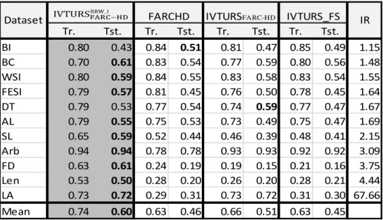
In this part of the study, the analysis is conducted in order to justify empirically the novelties introduced in our new proposal. To do so, we first compare the behavior of IVTURSRRW_I versus IVTURSFARC-HD and the two classifiers using type-1 FSs (FARC-HD algorithm and IVTURS_FS). In this way, we show the necessity of applying two of the three novelties introduced in the new proposal, namely, the use of IVFSs and the rescaling of the rule weight method.

Table 6 contains the results obtained when applying these four classifiers both in training and in testing. These results are measured using the geometric mean (Eq. (13)) and they are grouped by two columns to show the results obtained in training

This work was supported in part by the Spanish Ministry of Science and Technology under Project TIN2011-28488 and Project TIN2013-40765.

J. Sanz and H. Bustince are with the Department of Automática y Computación, Universidad Publica de Navarra, 31006 Pamplona, Spain (+34 948 166 408; fax: +34 948 168 924; e-mail: [email protected]; [email protected]).

D. Bernardo and H. Hagras are with the Computational Intelligence Centre, University of Essex, Wivenhoe Park, Colchester, UK.

F. Herrera is with the Department of Computer Science and Artificial Intelligence, Research Center on Information and Communications Technology (CITIC-UGR), University of Granada, 18071 Granada, Spain and with the Faculty of Computing and Information Technology - North Jeddah, King Abdulaziz University, 21589, Jeddah, Saudi Arabia (e-mail: [email protected]).

TABLE 6. RESULTS OBTAINED INTRAINING (TR.)

AND TESTING (TST.) MEASURED USING THE GEOMETRIC MEAN.

Tr. Tst. Tr. Tst. Tr. Tst. Tr. Tst. BI 0.80 0.43 0.84 0.51 0.81 0.47 0.85 0.49 1.15 BC 0.70 0.61 0.83 0.54 0.77 0.59 0.80 0.56 1.48 WSI 0.80 0.59 0.84 0.55 0.83 0.58 0.83 0.54 1.55 FESI 0.79 0.57 0.81 0.45 0.76 0.50 0.78 0.45 1.64 DT 0.79 0.53 0.77 0.54 0.74 0.59 0.77 0.47 1.67 AL 0.79 0.55 0.75 0.53 0.73 0.49 0.75 0.47 1.69 SL 0.65 0.59 0.52 0.44 0.46 0.39 0.48 0.41 2.15 Arb 0.94 0.94 0.78 0.78 0.93 0.93 0.92 0.92 3.09 FD 0.63 0.61 0.24 0.19 0.19 0.15 0.21 0.16 3.75 Len 0.53 0.50 0.28 0.20 0.26 0.20 0.28 0.21 4.44 LA 0.73 0.72 0.29 0.31 0.73 0.72 0.31 0.30 67.66 Mean 0.74 0.60 0.63 0.46 0.66 0.51 0.63 0.45

Dataset FARCHD IVTURSFARC-HD IVTURS_FS IR

(Tr.), in testing (Tst.). The best (highest) testing result is highlighted in bold-face.

From the results shown in Table 6 it is observed that our proposed approach, highlighted in grey, provides clearly the best mean result (of geometric mean) in testing (beating the competing techniques by a big margin followed by IVTURSFARC-HD) and it also reaches the best result in nine out of the eleven datasets. From these results we can stress two facts: on the one hand, the use of IVFSs (IVTURSRRW_I and IVTURSFARC-HD) allows the results of the approaches using type-1 FSs (FARC-HD and IVTURS_FS) to be improved and, on the other hand, it is observed that the rule weight rescaling method has a beneficial effect, since the results of

IVTURSRRW_I _{are better than those obtained when} applying IVTURSFARC-HD. The results of

IVTURSRRW_I _{are especially better than the ones} of the remainder approaches when the IR increases. Consequently, we can conclude that the new techniques introduced in our method are appropriate to deal with imbalanced data sets present in the vast majority of financial applications.

In order to support the superiority of

IVTURSRRW_I _{, we have applied the Friedman} aligned ranks test. The obtained ranks are shown in the third column of Table 7 and the p-value is 0.036, which implies the existence of statistical differences

among these four methods. This fact allows us to perform the Holm post-hoc test, whose obtained APVs are included in the last column of Table 7, to check whether IVTURSRRW_I , which is used as control method because it is the best ranked one, statistically outperforms the remainder approaches. Looking at the statistical results shown in Table 7, we can conclude that our new approach is statistically better than FARC-HD, IVTURSFARC-HD and IVTURS_FS and consequently, the use of both IVFSs and the rescaling rule weight method allows handling the imbalanced financial data sets to give a superior performance.

TABLE 7. HOLM'S TEST TO COMPARE IVTURS ä_å VERSUS FARC-HD, IVTURSFARC-HD AND IVTURS_FS.

IVTURS ä_å _{IS USED AS CONTROL METHOD.} No. Algorithm Ranking APV

1 IVTURS_FS 29.82 0.0011 2 FARCHD 28.27 0.0020 3 IVTURSFARC-HD 21.64 0.0380 4 IVTURS ä_å 10.27 -

Finally, we test the appropriateness of the proposed technique to deal with uncovered patterns. For the sake of generating specific fuzzy rules, we have run the fuzzy rule learning method using as maximum tree depth the number of attributes of the problem. For the FD dataset (we report only on this dataset as the similarity results are similar for the other datasets) we have selected the 10, 20, 30 and 40 fuzzy rules having a largest rule weight from each class, which implies obtaining rule bases composed of 20, 40, 60 and 80 rules respectively. The obtained results for the FD financial problem are presented in Table 8, where each row shows the number of rules in the rule base, the number of uncovered examples (using the rule base composed of as many rules as indicated in the first column) along with the accuracy achieved over the uncovered examples for each class (er_zX{| and ek_zX{|) and the result of the geometric mean (GM). It can be observed that the use of the similarity technique is beneficial for the system since when using the default rule the result of the geometric mean is always 0. Furthermore, it is noticed that the larger the number of fuzzy rules in the rule base the better the result of this technique is. This is due to the fact that when using a larger number of fuzzy rules the solution space is better covered leading to obtaining more suitable similar rules. This shows the power of proposed technique where we produce predictions for uncovered patterns to give a reasonable geometric mean.

TABLE 8 RESULTS OBTAINED WITH THE SIMILARITY TECHNIQUE ON THE FD DATASET USING THE

IVTURS ä_å _METHOD. Number of rules Number of uncovered examples erzX{| ekzX{| GM 20 1595 0.530 0.550 0.5399 40 933 0.570 0.590 0.5799 60 813 0.595 0.605 0.6000 80 315 0.602 0.638 0.6197

4.3Analyzing the suitability of

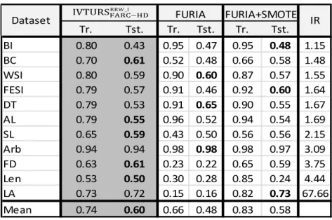
ÙÚÛÜÝ£_{ÞßÝà áâ}ÝÝã_Ù _{versus state-of-the-art} techniques

The second part of the experimental study is aimed at analyzing the behavior of our new proposal when it is compared versus state-of-the-art techniques that deal with imbalanced data. More specifically, we study the behavior of our approach versus the cost sensitive C4.5 decision tree [26] and

several classifiers that receive pre-processed data by means of SMOTE, which is one of the most widely used pre-processing techniques. To do so, this study is divided in three parts because we consider three types of algorithms, which are based on fuzzy association rules, the C4.5 decision tree and the FURIA algorithm, respectively.

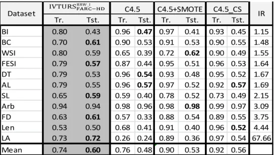
Table 9 shows the results obtained by our new method and the three classifiers based on the usage of fuzzy association rules using SMOTE both in training (Tr.) and in testing (Tst.), which are measured using the geometric mean. The best testing result for each dataset is highlighted in bold-face.

From results in Table 9, it is shown that the best mean testing result of geometric mean is provided by our new proposal. More specifically, we can observe that the results of the other method using IVFSs (IVTURSFARC-HD+SMOTE) are improved by 1.4% and the improvement versus the two approaches using type-1 FSs (FARCHD+SMOTE and IVTURS_FS+SMOTE) is around 3%.

In order to find whether there are statistical differences among these methods we have applied the aligned Friedman ranks test. The provided p-value is 0.0291, which confirms the existence of statistical differences where IVTURSRRW_I was the best method since it is the best ranked one (see third column of Table 10). Next, we have carried out the Holm’s post-hoc test to determine if

IVTURSRRW_I _{is statistically better than the} remainder methods. The results obtained in the statistical study are shown in Table 10, where it can be observed that our new proposal, which is used as control method because it obtains the best ranking, outperforms both the FARC-HD method and the fuzzy counterpart of the IVTURSFARC-HD algorithms using SMOTE (FARCHD+SMOTE and IVTURS_FS+SMOTE). Finally, it is noteworthy that there are not statistical differences with respect to IVTURSFARC-HD+SMOTE.

In the second part of the study we compare our proposed method against the approaches using decision trees, namely C4.5, C4.5 with SMOTE and the cost sensitive C4.5 (C45_CS), which widely used when dealing with imbalanced datasets. Table 11 shows the results provided by these four classifiers both in Training (Tr.) and testing (Tst.). It is noteworthy the notable improvement achieved by