A Hybrid Multi-objective Extremal Optimisation Approach for
Multi-objective Combinatorial Optimisation Problems
Pedro G´omez-Meneses, Marcus Randall and Andrew Lewis
Abstract— Extremal optimisation (EO) is a relatively recent
nature-inspired heuristic whose search method is especially suitable to solve combinatorial optimisation problems. To date, most of the research in EO has been applied for solving single-objective problems and only a relatively small number of attempts to extend EO toward multi-objective problems. This paper presents a hybrid multi-objective version of EO (HMEO) to solve multi-objective combinatorial problems. This new approach consists of a multi-objective EO framework, for the coarse-grain search, which contains a novel multi-objective combinatorial local search framework for the fine-grain search. The chosen problems to test the proposed method are the multi-objective knapsack problem and the multi-multi-objective quadratic assignment problem. The results show that the new algorithm is able to obtain competitive results to SPEA2 and NSGA-II. The non-dominated points found are well-distributed and similar or very close to the Pareto-front found by previous works.
I. INTRODUCTION
Nature-inspired methods like extremal optimisation (EO) have emerged in response to solve those optimisation prob-lems with which conventional mathematical techniques have difficulties. This may be as a result of the complex shape of their landscapes or the limitation of current computational systems. Most combinatorial optimisation problems (COPs) have been classified asN P-hard and new heuristics like EO are giving a new perspective on solving them instead of using traditional evolutionary algorithms (EAs). EO has the feature of requiring only one algorithm-specific parameter and it uses a minimal amount of memory, which can often lead to a lower computation time. At each iteration EO applies the principle of eliminating one of the weaker or less adapted solution components and replacing it by a random value.
Initially EO was applied to problems such as graph bi-partitioning, 3-colouring graph, spin-glass, and max-cut [1], [2]. Additionally, some exploratory work on other COPs such as the travelling salesman [3], [4], multidimensional knapsack [4], [5], maximum satisfiability [6], generalised assignment [7], bin packing [8], [9], [10], and dynamic problems [11] has been undertaken. Hybrid algorithms have also been developed in which aspects of EO are combined with other methods such as particle swarm optimisation [12], and genetic algorithms [13]. EO is now being extended to solve multi-objective problems [14], [15].
Pedro G´omez-Meneses is with the School of Information Technology, Bond University, QLD 4229, Australia (email: [email protected]) and also with the Departamento de Ingenier´ıa Inform´atica, Universidad Cat´olica de la Sant´ısima Concepci´on, Concepci´on, Chile (email: [email protected]).
Marcus Randall is with the School of Information Technology, Bond University, QLD 4229, Australia (email: [email protected]).
Andrew Lewis is with the Institute for Integrated and Intelligent Systems, Griffith University, Queensland, Australia (email: [email protected]).
A hybrid multi-objective extremal optimisation (HMEO) proposal is presented herein which finds solutions through the collaborative use of EO with a local search framework, both suitable (in principle) to solve a wide range of multi-objective combinatorial optimisation problems (MCOPs). The EO part of this approach carries out a coarse-grain search on the landscape that allows it to find new non-dominated points as the solution moves closer to the Pareto-front. The EO movement permits the exploration of the search space without becoming stuck in a particular region of the landscape. The local search part helps to develop a fine-grain movement to obtain a better approximation toward the Pareto-front as well as to produce a greater diversification of the points towards the ends of the Pareto-front. The advantage of this proposal is its simplicity of implementation due to its single parameter and selection procedure.
Given this new approach, we test the behaviour of HMEO on two MCOPs. They are the multi-objective knapsack problem (MKP) and the multi-objective quadratic assignment problem (MQAP). The results show that the new hybrid multi-objective algorithm works well with respect to con-vergence and distribution of solutions. Thus, HMEO can be a potential choice to efficiently solve MCOPs.
The paper is organised as follows. Section 2 gives a summary of EO. Section 3 introduces the basic concepts of multi-objective problems and Pareto optimality. Section 4 presents two benchmark problems to validate the proposal. Section 5 explains the HMEO framework to solve MCOPs. Section 6 shows the results obtained and presents an analysis of them. Finally, in Section 7 we conclude and discuss the future work arising from this study.
II. EXTREMALOPTIMISATION
EO is an evolutionary meta-heuristic proposed by Bak and Sneppen [16] based on a model of co-evolution be-tween species. This model describes species’ evolution via extinction events as a self-organised critical (SOC) [17] process. SOC tries to explain the manifestation of complex phenomena in nature such as the formation of sand piles and the occurrences of earthquakes [18]. The main characteristic is that a power law describes the events in the system. Simply put, these systems have some critical points that are configured in a particular way. When an event converges towards one of these points, a critical state is reached which triggers a series of changes over the elements near to the critical point. Using self-organisation the system is able to reach a new state of equilibrium. Finally, it evolves in a WCCI 2010 IEEE World Congress on Computational Intelligence
transient period of stability until the next critical point is reached.
A good way to understand EO’s characteristics is to compare it with another well-known method such as genetic algorithms (GAs) [19]. First, a GA commonly has a set of parameters that need to be tuned for proper operation; however, in EO only one specific parameter must be tuned. Second, in EO the fitness value is not calculated for each structure that represents a solution as in a GA but for each component of the structure. Each component is evaluated according to its contribution in obtaining the best solution. Third, canonical EO works with a single solution instead of a population of solutions as in GA. Last, EO modifies the worst part of the solution while in contrast GA promotes a group of elite solutions.
There is only one EO specific parameter that is often referred to asτ [20]. This parameter is used probabilistically to choose the component value to be changed at each iteration of the algorithm. The algorithm ranks the components and assigns to them a number from 1 ton using the fitness of each one (where n is the number of components). There-fore, the fitness must be sorted from the worst to the best evaluated. Then a selection method such as roulette wheel (RWS) is used to choose the component whose value will be changed to a random value according to the probability calculated for each component as shown in Equation 1. If the new component makes the solution the best found so far, according to the evaluation function, then this solution is saved asXbest. The EO process is shown in Algorithm 1.
Pi=i−τ ∀i 1≤i≤n, τ≥0 (1)
where:
n is the total number of components evaluated and ranked, and
Pi is the probability that theithcomponent is chosen.
Algorithm 1 Standard EO for minimisation problem
Generate an initial random solutionX=(x1, x2, . . . , xn); SetXbest=X;
Generate the probabilities arrayP according to Equation 1; for a preset number of iterations do
Evaluate and rank fitnessλifor eachxifrom worst to best,1≤i≤n; Select componentjbased on the probability of its rankPiusing RWS;
xj=Generate a random appropriate value that is not equal toxj;
Eva(X) =Evaluate the new solution; ifEva(X)< Eva(Xbest)thenXbest=X; end for
ReturnXbestandEva(Xbest);
III. MULTI-OBJECTIVEOPTIMISATIONPROBLEMS
Many real-world optimisation problems have several op-tima (maximum or minimum). These opop-tima are equally important, either by having the same numerical value, or because they are not able to establish a criterion to decide which of them is better. Normally, for multi-objective opti-misation problems (MOPs), the decision concerning the most appropriate solution is a contextual one and is often left to a human decision-maker.
Multi-objective optimisation can be defined as the chal-lenge of discovering a collection of solutions that satisfies all constraints at the same time and maximises or minimises each one of the objective functions. Generally these objective functions are in conflict with each other in terms of their evaluation. Therefore, a multi-objective optimisation problem must find a set of solutions that optimise all the objective functions for a particular problem.
The multi-objective optimisation approach resembles single-objective optimisation. The problem is to find a so-lution vector~xsuch that:
Minimise/Maximise ~f(~x)
~x∈̥⊆R where:
~x is a vector of decision variables(x1, ..., xn)that represents a solution,
~
f(~x) is a vector of objective functions(f1(~x), ..., fk(~x))to be maximised or minimised,
̥ is the feasible search space limited by the constraints,
R is the entire search space.
The more accepted concept of optimality in a multi-objective field is the so-called Pareto optimality. This notion is based on the concept of dominance which is defined below [21].
Definition 1 (Pareto Dominance): For a minimisation
problem, a solution~sdominates another solution ~s′, if and only if, ~s is partially less than ~s′ and there exists at least an objective where~sis absolutely less than ~s′, denoted by
~s≺~s′.
Once the concept of Pareto dominance has been defined an explanation about when a solution is a Pareto-optimal is given next.
Definition 2 (Pareto-optimal): A solution ~s∗ is
Pareto-optimal, if and only if, there is no other solution~s which dominates it. That is,∄~s∈̥:~s≺ ~s∗.
After some optimisation process several Pareto-optimal solutions may be found. The set of results that gathers all of the Pareto optimal solutions is known as the Pareto optimal set (P∗).
Definition 3 (Pareto optimal set): The Pareto optimal set
(P∗) is the set of all Pareto optimal solutions ~s∗ such that there is not a solution~sthatf(~s)≺f(~s∗).
The person that chooses the final solutions from the Pareto optimal set for a particular problem is the decision-maker. The vector that satisfies these definitions is known as the Pareto-front. Thus, for a given multi-objective problem ~f(~x) and a set of Pareto-optimal solutionsP∗, the Pareto-front is defined below.
Definition 4 (Pareto-front): Pareto-front P F∗ is the set
P∗ of all solutions that are Pareto-optimal for a given
problem ~f(~x).
IV. BENCHMARKPROBLEMS
This section presents a concise description of two repre-sentative MCOPs classified asN P-hard which are used to validate the proposed method. These are the multi-objective knapsack problem and the multi-objective quadratic assign-ment problem.
A. Multi-objective Knapsack Problem
The knapsack problems (KP) has widely been used as a benchmark problem to compare new general purpose meta-heuristics. Also, we can find several real-world problems that can be modelled by a KP, specially those that must assign a series of items linked with a profit and cost to a resource (knapsack) with limited capacity [22]. The idea is to maximise the profit without overloading the resource capacity.
The multi-objective version of the classical 0/1 KP can be obtained by adding more knapsacks to the problem. Formally, it can be represented as:
Maximisef~(~x) ={f1(~x), f2(~x), . . . , fm(~x)} with fj(~x) = Xn i=1 pijxi, ∀j 1≤j≤m Subject to n X i=1 wijxi≤cj, ∀j 1≤j≤m xi∈ {0,1}, ∀i 1≤i≤n where:
pij is the profit of itemiin knapsackj,
wij is the weight of itemiin knapsackj,
cj is the capacity of the knapsackj,
~x is the solution vector(x1, x2, . . . , xn), and
xi is theithdecision variable in the solution vector, 1 if the item is in the solution, 0 otherwise.
B. Multi-objective Quadratic Assignment Problem
The quadratic assignment problem occurs in applications such as layout of malls, hospitals and airport terminals, location of electronic components in an integrated circuit, distribution of resources in a collection centre and any other case where it is necessary to assign a set of facilities to specific locations. The objective is to minimise the cost associated with the flows of items amongst facilities and the distance between these.
When we have two or more different kinds of flows or facilities that must be assigned to a location then we are working with a MQAP. For instance, in a hospital we want to simultaneously minimise the flow of doctors, patients, nurses, visitors, equipment, and so on.
Formally, the MQAP can be represented as:
MinimiseC~(~π) ={C1(~π), C2(~π), . . . , Cm(~π)}, ¯π∈Ω with Ck(~π) =Xn i=1 n X j=1 bk ijaπiπj, 1≤k≤m where:
m is the number of objectives or flows,
n is the number of facilities/locations,
πi is the location of facilityiin permutation~π, Ω is the set of all permutations,
bk
ij is thekthflow from facilityito facilityj, and
aπiπj is the distance between location of facilityi
and location of facilityj.
V. HYBRIDMULTI-OBJECTIVEEO
Previous research applying EO to COPs has shown the advantages of complementing EO with a local search mech-anism [5], [8], [9], [10]. This section shows how HMEO is implemented to deal with MCOPs. First, the multi-objective combinatorial local search framework (MCLS) will be de-scribed and then the multi-objective EO framework.
A. Multi-objective Combinatorial Local Search Framework
Most multi-objective local search methods in the literature use genetic algorithms. For these, the two approaches more often developed are based on Pareto ranking and weighted scalar fitness functions [23]. Comparative studies showing the advantages and disadvantages of both techniques can be found in Ishibuchi and Narukawa [23] and Jaszkiewicz [24]. Because our area of interest is focused on combinatorial problems, our goal in this paper is to discover novel ideas that can be applied in a general way to MCOPs. Observing the previous analysis of the two local search techniques used in evolutionary multi-objective optimisation (EMO) we contribute a new, simpler approach in a effort to offer a new alternative to be used for MCLS.
The MCLS framework proposed is simple. Modifying and mixing the concepts of the weighted scalar fitness and the lexicographic ordering we decide to change the weighted vector by a probability vector which is filled with random valuesP(m)rand ∼U(1,0). This vector is used to choose an objective based on its assigned probabilityPiusing RWS. As most combinatorial problems explore the neighbourhood of the landscape using a swap operator through a double traverse of the solution vector, a single local search on the objective chosen will be done by each single traverse of the solution vector. Before each single traverse is started, a new objective function is selected which could be the same as before. Finally, if the local search finds a better solution for a particular objective then the non-dominance procedure is called to see if the new solution should be added to the attainment surface. Algorithm 2 shows the pseudocode of the MCLS procedure.
The details for the single local search implementation are given for the MKP in G´omez-Meneses and Randall [5] and for the MQAP in Ramkumar, Ponnambalam and Jawa-har [25].
Algorithm 2 Pseudocode of the MCLS procedure
Require: m=number of objective functions
Require: n=number of elements of the solution vector Require: ~S=solution vector
Generate a random variate vectorP(m)rand∼U(1,0); for a traverse of ~Susing indexido
Select an objective using RWS and theP(m)randprobability; for a traverse of ~Susing indexjdo
Swap the elementsiandjof ~S;
if the~Snewfeasible and better than the current solution then
P Set= non-dominance(~Snew); end for
end for
B. Multi-objective EO framework
One of the main characteristics of EO is its ability to locate a possible optimal solution stochastically in search space. This characteristic enables EO to avoid being trapped in a local minimum; however, this characteristic also hinders EO from being able to refine the search when a solution is near the optimal result. Therefore, MHEO is made up of an multi-objective EO framework and a MCLS framework that is executed every time a feasible solution is found.
MHEO starts by generating an initial random solution ~S. If the solution is feasible then this becomes the first point of the attainment surface.
The solution in EO can move between feasible and in-feasible space (see Randall [7]) according to the problem being solved. For instance, the MQAP only generates feasible solutions. In this case, the infeasible component of the framework is not considered. Thus, it is necessary to carry out an appropriate multi-objective EO selection process for both cases.
When the solution is feasible, the fitness calculation is focused on locating which part of the solution adversely affects its quality the most. However, when the solution is infeasible, the fitness calculation is focused on locating which part of the solution is more responsible for the violation of one or more constraints. Thus, the extension from the single EO to the multi-objective EO is given by the simple scalar addition of the fitness of each objective function in the problem to solve. λi(~x) = n X j=1 λji(~x), ∀i 1≤i≤n where:
m is the number of objectives,
n is the number of solutions component,
λi is the multi-objective fitness of theith com-ponent, and
λji is the single-objective fitness of theith
com-ponent.
After calculating the fitness of the solution, the compo-nents are ranked from worst to best. Then one of them is selected, based on the probability of its rankPi using RWS, to change its value. As previously mentioned, the new value is chosen at random, but within the legal scope of values.
Next, the new solution is accepted and evaluated to see if it is feasible or not. In the case a feasible solution is
obtained, the non-dominance procedure is called to see if the new solution should be added to the attainment surface. Finally, at preset intervals throughout the execution of the multi-objective EO process, the local search is invoked by the process described in the previous section to refine the search. The reason for running the MCLS at regular intervals is to complement both frameworks. On one hand, the multi-objective EO component is concentrated in the central part of the Pareto-front. On the other hand, when the MCLS component is activated, the solution is shifted towards the ends of the Pareto-front.
Algorithm 3 shows the pseudocode of the HMEO model for MCOPs.
Algorithm 3 Pseudocode of the HMEO model for MCOP
Generate an initial random solution~S; if the current solution is feasible then
Add ~SintoP Set;
Generate the probabilities array P according to Equation 1; forg= 1toNumIterdo
if the current solution is feasible then
Evaluate fitness~λaccording to feasible current solution; else
Evaluate fitness~λaccording to infeasible current solution;; Rank fitnessλifor eachSifrom worst to best,1≤i≤n; SelectSjbased on the probability of its rankPiusing RWS; Choose~Snew in the neighbourhood of~S whereSj’s value changes to a random one;
if~Snewis feasible then
P Set= non-dominance(~Snew); if(int)(g/(NumIter/100))%2)then
Local Search(); end for
VI. COMPUTATIONALEXPERIMENTS
The proposed HMEO method was coded in the C lan-guage and compiled with gcc version 4.4.1. The computing platform used to perform the tests has a 1.86 GHz Intel Core2 CPU and 917 MB of memory, running under Linux.
HMEO is configured to run 10 test trials varying by random seed. The number of iterations to complete a HMEO process is 500000 for MKP and 100000 for MQAP. Tests performed with a larger number of iterations, for each problem, reported no significant improvements in results. The difference in the number of iterations is due to the local search technique used in each. The local search for the MQAP is more exhaustive than that used in MKP. For this reason MQAP requires fewer iterations. Theτ parameter is set at 1.4 which has been reported in previous research [8], [7], [26] as being a good value to obtain efficient solutions.
A. Test Problems
In the first of the experiments HMEO is applied to solve a group of six different MKPs from Zitzler and Thiele [27]. The problem’s name is presented through the nomenclature KS.nnn.m where nnn is the number of items and m is the number of objectives. The test problems and test data were obtained from Zitzler and Laumanns [28]. For the first four problems KS.100.2, KS.250.2, KS.500.2 and KS.100.3 we compare the results with the true Pareto-optimal set
(POS) which is available from this source. For the last two problems KS.750.2, KS.750.3 we compare the results with those obtained by Strength Pareto Evolutionary Algorithm 2 (SPEA2) and Non-Dominated Sorting Genetic Algorithm II (NSGA-II). The reason for this particular selection of problems and benchmark of comparison was subject to the availability of experimental results from the source.
The profit and weight arrays are formed by uncorrelated random integers in the interval [10,100]. The knapsack capacity is set to half the total weight of all items with respect to a particular knapsack. That is:
ci= 0.5 m X j=1
wij
In the second, HMEO is applied to solve a group of eight different MQAPs by Knowles and Corne [29]. These test problems have 10 facilities/locations with two objectives that correspond to a 2 flow matrix. Three out of eight instances were created using a uniformly random instance generator and the other five instances were created using a real-like instance generator. The problem’s name is presented through the nomenclature KCnn-mfl-itypewhere nnis the number of facilities/locations, m is the number of objectives or flows and itype is the instance identification starting with a correlative number plus the instance generator used (uni for uniformly random andrlfor real-like). The test problems and test data were obtained from Knowles [30], along with the true Pareto-optimal sets for the eight test problems having 10 facilities/locations instances. Our results are compared against those solution sets.
B. Results
The three basic concepts that we considered for multi-objective optimisation are:
1) Minimise the convergence - that is the Pareto-front distance produced by our proposal with respect to the true Pareto-front (assuming that it is known).
2) Maximise the diversity - that is the distribution of so-lutions, so that we can have a Pareto-front distribution as uniform as possible.
3) Maximise the coverage - that is to extend the Pareto-front solutions toward the furthest areas of the land-scape.
In the first of the experiments describes the results when HMEO is applied to solve the MKP.
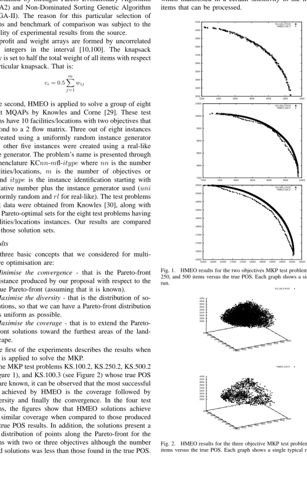
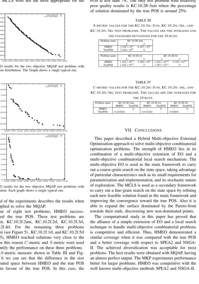
For the MKP test problems KS.100.2, KS.250.2, KS.500.2 (see Figure 1), and KS.100.3 (see Figure 2) whose true POS results are known, it can be observed that the most successful feature achieved by HMEO is the coverage followed by the diversity and finally the convergence. In the four test problems, the figures show that HMEO solutions achieve a quite similar coverage when compared to those produced by the true POS results. In addition, the solutions present a regular distribution of points along the Pareto-front for the problems with two or three objectives although the number of found solutions was less than those found in the true POS.
However, HMEO showed a degradation in the convergence as the number of variables increased from 100 to 500 items which manifested in a certain sensitivity to the number of items that can be processed.
3200 3300 3400 3500 3600 3700 3800 3900 4000 4100 3200 3400 3600 3800 4000 4200 4400 "KS.100.2.POS" "HMEO.100.2" 7500 8000 8500 9000 9500 10000 10500 7000 7500 8000 8500 9000 9500 10000 "KS.250.2.POS" "HMEO.250.2" 16000 16500 17000 17500 18000 18500 19000 19500 20000 20500 15500 16000 16500 17000 17500 18000 18500 19000 19500 20000 20500 "KS.500.2.POS" "HMEO.500.2"
Fig. 1. HMEO results for the two objectives MKP test problems with 100, 250, and 500 items versus the true POS. Each graph shows a single typical run. 2600 2800 3000 3200 3400 3600 3800 4000 4200 2600 2800 3000 3200 3400 3600 3800 4000 4200 2600 2800 3000 3200 3400 3600 3800 4000 4200 "KS.100.3.POS" 2600 2800 3000 3200 3400 3600 3800 4000 4200 2600 2800 3000 3200 3400 3600 3800 4000 4200 2600 2800 3000 3200 3400 3600 3800 4000 4200 "HMEO.100.3"
Fig. 2. HMEO results for the three objective MKP test problems with 100 items versus the true POS. Each graph shows a single typical run.
22000 23000 24000 25000 26000 27000 28000 29000 30000 31000 23000 24000 25000 26000 27000 28000 29000 30000 31000 "SPEA2" "NSGA2" "HMEO"
Fig. 3. HMEO results for the two objective MKP test problems with 750 items (KS.750.2) versus SPEA2 and NSGA-II. This graph shows a single typical run. 23000 24000 25000 26000 27000 28000 29000 30000 31000 32000 22000 23000 24000 25000 26000 27000 28000 29000 30000 31000 22000 24000 26000 28000 30000 32000 "HMEO" 23000 24000 25000 26000 27000 28000 29000 30000 31000 32000 22000 23000 24000 25000 26000 27000 28000 29000 30000 31000 22000 24000 26000 28000 30000 32000 "SPEA2" 23000 24000 25000 26000 27000 28000 29000 30000 31000 32000 22000 23000 24000 25000 26000 27000 28000 29000 30000 31000 22000 24000 26000 28000 30000 32000 "NSGA2"
Fig. 4. HMEO results for the three objective MKP test problems with 750 items (KS.750.3) versus SPEA2 and NSGA-II. Each graph shows a single typical run.
For the problems KS.750.2 (see Figure 3) and KS.750.3 (see Figure 4), which are compared against the well known methods SPEA2 and NSGA-II, it can be observed again that the most successful feature achieved by HMEO is coverage. By inspection of the figures it may be seen that in both test problems the area or surface covered by the Pareto front obtained with the proposed algorithm is broader than those found by SPEA2 and NSGA-II. Diversity worked quite well for the test problem with two objectives but for the test problem with three objectives shows some surface areas without solutions. If we compare the distribution of points
between test problems KS.100.3 and KS.750.3 it can be inferred that the greater the number of items, the greater the difficulty to achieve a uniform distribution of points. It is interesting to note that the convergence seems to be the weak point of the implementation to solve the MKP through HMEO framework. Despite reaching an attainment surface very close to those achieved by SPEA2 and NSGA-II, only a few points dominate those of SPEA2.
A better way to show the analysis for the test problems KS.750.2 and KS.750.3 is by presenting some metrics that help us to reinforce the information presented in Figures 3 and 4. Thus, the S-metric and C-metric proposed by Zit-zler [31] are presented. The S-metric measures how much of the objective space is dominated by a given non-dominated Pareto-setA. This metric is useful to measure the coverage of a solution in an independent way. A high value of this metric means a wide coverage of the Pareto-set under analysis. On the other hand, using the C-metric (coverage) two Pareto-sets can be compared to each other. The nomenclature used is C(A, B) and the interpretation is as follows. The value
C(A, B) = 1 means that all solutions inB are dominated by A. The value C(A, B) = 0 represents the situation where none of the solutions in B are dominated by A. Both orderings have to be considered since C(A, B) is not necessarily equal to 1− C(B, A). A more detailed explanation of these metrics can be found in Knowles and Corne [32].
TABLE I
S-METRIC VALUES FOR THEKS.750.2ANDKS.750.3TEST PROBLEMS. THE VALUES ARE THE AVERAGES AND THE STANDARD DEVIATIONS FOR
THE10RUNS. Problem name KS.750.2 KS.750.3 ¯ χ σ χ¯ σ HMEO 3.86941∗107 5.37987∗104 2.33542∗1011 5.11311∗108 SPEA2 3.48117∗107 3.54090∗105 1.91337∗1011 1.94082∗109 NSGA-II 3.34971∗107 4.05495∗105 1.82142∗1011 2.07875∗109 TABLE II
C-METRIC VALUES FOR THEKS.750.2ANDKS.750.3TEST PROBLEMS. THE VALUES ARE THE AVERAGES FOR THE10RUNS.
Problem name KS.750.2 KS.750.3 HMEO SPEA2 NSGA-II HMEO SPEA2 NSGA-II HMEO - 0.0828 0.02264 - 0.5977 0.87957 SPEA2 0.45518 - 0.17572 0.07739 - 0.7961 NSGA-II 0.40276 0.64536 - 0.00872 0.0169
-From Table I we can see that HMEO achieves a better coverage of the dominated space on KS.750.2 and KS.750.3. These results concur with Figures 3 and 4. By reference to Table II, we can observe that for the test problem KS.750.2 HMEO dominates only a reduced number of solutions of SPEA2 and NSGA-II. However, 40% to 45% of solutions from HMEO are not dominated by either of the two other methods (SPEA2, NSGA-II). In the case of KS.750.3, the table shows that HMEO dominates around 60% of the solu-tions of SPEA2 and 88% of NSGA-II, and less than 1% of HMEO solution are dominated by either SPEA2 or NSGA-II. The latter represents a significantly better performance of
HMEO above SPEA2 or NSGA-II.
Finally, the inferior results obtained in convergence sug-gests that either the criterion to calculate the fitness for the multi-objective EO framework or the local search technique used for the MCLS were not the most appropriate for the MKP. 170000 180000 190000 200000 210000 220000 230000 240000 250000 260000 270000 280000 190000 200000 210000 220000 230000 240000 250000 260000 270000 280000 290000 300000 "KC10-2fl-3uni.PO" "KC10-2fl-3uni.HMEO"
Fig. 5. HMEO results for the two objective MQAP test problem with uniformly random distribution. The Graph shows a single typical run.
2e+006 2.5e+006 3e+006 3.5e+006 4e+006 4.5e+006 5e+006 5.5e+006 6e+006
1.5e+006 2e+006 2.5e+006 3e+006 3.5e+006 4e+006 4.5e+006 5e+006 5.5e+006 6e+006 "KC10-2fl-1rl.PO" "KC10-2fl-1rl.HMEO" 2e+006 4e+006 6e+006 8e+006 1e+007 1.2e+007 1.4e+007 1.6e+007 1.8e+007 2e+007
2e+006 3e+006 4e+006 5e+006 6e+006 7e+006 8e+006 9e+006 1e+007 1.1e+007 "KC10-2fl-5rl.PO" "KC10-2fl-5rl.HMEO"
Fig. 6. HMEO results for the two objective MQAP test problems with real-like distribution. Each graph shows a single typical run.
The second of the experiments describes the results when HMEO is applied to solve the MQAP.
In five out of eight test problems, HMEO success-fully achieved the true POS. These test problems are KC.10.2f.1uni, KC.10.2f.2uni, KC.10.2f.2rl, KC.10.2f.3rl, and KC.10.2f.4rl. For the remaining three problems KC.10.2f.3uni (see Figure 5) , KC.10.2f.1rl, and KC.10.2f.5rl (see Figure 5), HMEO reached solutions very close to the true POS. For this reasonC-metric andS-metric were used again to quantify the performance on these three problems. From the S-metric measure shown in Table III and Fig-ures 5, and 6 we can see that the difference in the size of the dominated space between HMEO and the true POS is minimal in favour of the true POS. In this case, the
convergence, diversity, and coverage features work quite well. A similar situation can be observed when theC-metric data in Table IV are analysed. For the two like-real test problems the percentage of solutions dominated by the true POS is less than 7%. The only test problem with relatively poor quality results is KC.10.2fl-3uni where the percentage of solution dominated by the true POS is around 25%.
TABLE III
S-METRIC VALUES FOR THEKC.10.2FL-3UNI, KC.10.2FL-1RL,AND
KC.10.2FL-5RL TEST PROBLEMS. THE VALUES ARE THE AVERAGES AND THE STANDARD DEVIATIONS FOR THE10RUNS.
Problem name KC.10.2fl-3uni
¯ χ σ HMEO 5.358∗109 6.407∗106 TruePOS 5.382∗109 0 Problem name KC.10.2fl-1rl KC.10.2fl-5rl ¯ χ σ χ¯ σ HMEO 1.162∗1013 1.893∗109 1.305∗1014 3.739∗1010 TruePOS 1.162∗1013 0 1.307∗1014 0 TABLE IV
C-METRIC VALUES FOR THEKC.10.2FL-3UNI, KC.10.2FL-1RL,AND
KC.10.2FL-5RL TEST PROBLEMS. THE VALUES ARE THE AVERAGES FOR THE10RUNS.
Problem name KC.10.2fl-3uni KC.10.2fl-1rl KC.10.2fl-5rl HMEO TruePOS HMEO TruePOS HMEO TruePOS HMEO - 0 - 0 - 0
TruePOS 0.245924 - 0.014232 - 0.06605
-VII. CONCLUSIONS
This paper described a Hybrid Multi-objective Extremal Optimisation approach to solve multi-objective combinatorial optimisation problems. The strength of HMEO lies in its combination of a multi-objective extension of EO and a multi-objective combinatorial local search mechanism. The multi-objective EO is used as the main framework to carry out a coarse-grain search on the state space, taking advantage of particular characteristics such as its small requirements for parametrisation and implementation, and its stochastic nature of exploration. The MCLS is used as a secondary framework to carry out a fine-grain search on the state space by refining each new feasible solution found in the main framework and improving the convergence toward the true POS. Also it is able to expand the surface dominated by the Pareto-front towards their ends, discovering new non-dominated points.
The computational study in this paper has proved that the alliance of a simple extension of EO and a local search technique to handle multi-objective combinatorial problems is competitive and efficient. Thus, HMEO demonstrated a similar coverage when it was compared with the true POS and a better coverage with respect to SPEA2 and NSGA-II. The achieved diversification was acceptable for most problems. The best results were obtained with MQAP, having an almost perfect output. The MKP experiments performance better for larger problems. HMEO was competitive with the well known multi-objective methods SPEA2 and NSGA-II.
The results reported in this paper are preliminary, but promising. Future work will include a series of transforma-tions of the MEO framework to improve the performance of the HMEO approach. First, the fitness calculation will be changed to an evaluation based on the Pareto-dominance concept, which is popularly used by many existing multi-objective evolutionary algorithms. Second, a population-based extension of HMEO will be developed. These two steps will be implemented with the objective of improving the diversity and convergence of the current approach. A new series of experiments will be executed to solve more complex test problems than MKP and MQAP, as well as to solve new benchmark problems such as the Multi-objective Flow-shop Scheduling Problem, the Multi-objective Travelling Sales-man Problem and the Multi-objective Solid Transportation Problems.
REFERENCES
[1] S. Boettcher, “Extremal optimization for Sherrington-Kirkpatrick spin glasses,” The European Physical Journal B, vol. 46, pp. 501–505, 2005.
[2] S. Boettcher and A. Percus, “Extremal optimization: An evolutionary local-search algorithm,” in8thINFORMS Computer Society Confer-ence, 2003.
[3] S. Boettcher and A. G. Percus, “Evolutionary strategies extremal optimization: Methods derived from co-evolution,” in GECCO-99:
Proceedings of the Genetic and Evolutionary Computation Conference,
1999, pp. 825–832.
[4] M. Randall and A. Lewis, “An extended extremal optimisation model for parallel architectures,” in 2nd International Conference on e-Science and Grid Computing, 2006.
[5] P. G´omez-Meneses and M. Randall, “Extremal optimisation with a penalty approach for the multidimensional knapsack problem,” in
SEAL, ser. Lecture Notes in Computer Science, vol. 5361. Springer, 2008, pp. 229–238.
[6] M. E. Mena¨ı and M. Batouche, “An effective heuristic algorithm for the maximum satisfiability problem,” Applied Intelligence, vol. 24, no. 3, pp. 227–239, 2006.
[7] M. Randall, “Enhancements to extremal optimisation for generalised assignment,” in ACAL, ser. Lecture Notes in Artificial Intelligence, vol. 4828. Springer, November 2007, pp. 369–380.
[8] T. Hendtlass and M. Randall, “Extremal optimisation and bin packing.” in SEAL, ser. Lecture Notes in Computer Science, vol. 5361. Springer, 2008, pp. 220–228. [Online]. Available: http://dblp.uni-trier.de/db/conf/seal/seal2008.html
[9] M. Randall, T. Hendtlass, and A. Lewis, “Extremal optimisation for assignment type problems,” in Biologically-Inspired Optimisation Methods: Parallel Algorithms, Systems and Applications, ser. Studies in Computational Intelligence. Springer-Verlag, 2009, vol. 210, pp. 139–164. [Online]. Available: http://www.springer.com/engineering/book/978-3-642-01261-7 [10] P. G´omez-Meneses and M. Randall, “A hybrid extremal optimisation
approach for the bin packing problem,” in ACAL, ser. Lecture Notes in Computer Science, K. B. Korb, M. Randall, and T. Hendtlass, Eds., vol. 5865. Springer, 2009, pp. 242–251.
[11] T. Hendtlass, I. Moser, and M. Randall, “Dynamic problems and nature inspired meta-heuristics,” in2ndIEEE International Conference on e-Science and Grid Computing, 2006.
[12] M. R. Chen, Y. Z. Lu, and Q. Luo, “A novel hybrid algorithm with marriage of particle swarm optimization and extremal optimization,”
Optimization Online, 2007.
[13] Y. W. Chen, Y. Z. Lu, and G. K. Yang, “Hybrid evolutionary algorithm with marriage of genetic algorithm and extremal optimization for pro-duction scheduling,” International Journal of Advanced Manufacturing
Technology, 2007.
[14] M.-R. Chen, Y.-Z. Lu, and G. Yang, “Multiobjective optimization using population-based extremal optimization,” Neural Computing &
Applications, April 2007.
[15] M.-R. Chen and Y.-Z. Lu, “A novel elitist multiobjective optimization algorithm: Multiobjective extremal optimization,” European Journal
of Operational Research, vol. 127, no. 3, pp. 637–651, August 2008.
[16] P. Bak and K. Sneppen, “Punctuated equilibrium and criticality in a simple model of evolution,” Physical Review Letters, vol. 71, no. 24, pp. 4083–4086, 1993.
[17] P. Bak, C. Tang, and K. Wiesenfeld, “Self-organized criticality: An explanation of the 1/f noise,” Physical Review Letters, vol. 59, no. 4, pp. 381–384, 1987.
[18] P. Bak, How nature works. Springer-Verlag New York Inc., 1996. [19] D. E. Goldberg, Genetic Algorithms in Search, Optimization and
Machine Learning. Boston, MA, USA: Addison-Wesley Longman Publishing Co., Inc., 1989.
[20] S. Boettcher, “Extremal optimization: Heuristics via co-evolutionary avalanches,” Computing in Science and Engineering, vol. 2, pp. 75– 82, 2000.
[21] C. Coello-Coello, G. B. Lamont, and D. A. V. Veldhuizen,
Evolution-ary Algorithms for Solving Multi-Objective Problems, Second ed., ser.
Genetics and Evolutionary Computation, D. E. Goldberg and J. R. Koza, Eds. Springer, 2007.
[22] M. Vasquez and Y. Vimont, “Improved results on the 0-1 multi-dimensional knapsack problem,” European Journal of Operational
Research, vol. 165, no. 1, pp. 70–81, August 2005. [Online].
Available: http://ideas.repec.org/a/eee/ejores/v165y2005i1p70-81.html [23] H. Ishibuchi and K. Narukawa, “Some issues on the implementation of local search in evolutionary multiobjective optimization,” in
Genetic and Evolutionary Computation, GECCO 2004, ser. Lecture
Notes in Computer Science, vol. Volume 3102/2004. Springer Berlin / Heidelberg, 2004, pp. 1246–1258. [Online]. Available: http://www.springerlink.com/content/1GDAWYGAGT55RKW5 [24] A. Jaszkiewicz, “Genetic local search for multi-objective combinatorial
optimization,” European Journal of Operational Research, vol. 137, no. 1, pp. 50–71, February 2002. [Online]. Available: http://ideas.repec.org/a/eee/ejores/v137y2002i1p50-71.html
[25] A. S. Ramkumar, S. G. Ponnambalam, and N. Jawahar, “A new iterated fast local search heuristic for solving qap formulation in facility layout design,” Robot. Comput.-Integr. Manuf., vol. 25, no. 3, pp. 620–629, 2009.
[26] S. Boettcher and A. G. Percus, “Extremal optimization for graph partitioning,” Physical Review E, vol. 64, p. 026114, 2001. [27] E. Zitzler and L. Thiele, “Multiobjective evolutionary algorithms: a
comparative case study and the strength pareto approach,”
Evolution-ary Computation, IEEE Transactions on, vol. 3, no. 4, pp. 257–271,
Nov 1999.
[28] E. Zitzler and M. Laumanns, “Test problem suite,” In web page accessed on January 2010. [Online]. Available: http://www.tik.ee.ethz.ch/sop/download/supplementary/testProblemSuite [29] J. D. Knowles and D. Corne, “Instance generators and test
suites for the multiobjective quadratic assignment problem,” in EMO, ser. Lecture Notes in Computer Science, C. M. Fonseca, P. J. Fleming, E. Zitzler, K. Deb, and L. Thiele, Eds., vol. 2632. Springer, 2003, pp. 295–310. [Online]. Available: http://www.springerlink.com/content/t57tg2dek0k77lx7/
[30] J. Knowles, “The multiobjective quadratic assignment problem (mqap),” In web page accessed on January 2010. [Online]. Available: http://dbkgroup.org/knowles/mQAP/
[31] E. Zitzler, “Evolutionary Algorithms for Multiobjective Optimization: Methods and Applications,” Ph.D. disserta-tion, ETH Zurich, Switzerland, 1999. [Online]. Available: http://www.tik.ethz.ch/ sop/publications/
[32] J. Knowles and D. Corne, “On metrics for comparing nondominated sets,” in Evolutionary Computation, 2002. CEC ’02. Proceedings of