Repositorio Institucional de la Universidad Autónoma de Madrid https://repositorio.uam.es
Esta es la versión de autor del artículo publicado en:
This is an author produced version of a paper published in:
Scandinavian Journal of Statistics 38.3 (2011): 480-498 DOI: http://dx.doi.org/10.1111/j.1467-9469.2011.00734.x
Copyright: © 2011 Board of the Foundation of the Scandinavian Journal of Statistics El acceso a la versión del editor puede requerir la suscripción del recurso
Supervised classification for a family of Gaussian
functional models
Amparo Ba´ıllo
∗, Juan Antonio Cuesta-Albertos
†and Antonio Cuevas
∗∗Universidad Aut´onoma de Madrid and†Universidad de Cantabria
Abstract
In the framework of supervised classification (discrimination) for functional data, it is shown that the optimal classification rule can be explicitly obtained for a class of Gaussian processes with “triangular” covariance functions. This explicit knowledge has two practical consequences. First, the consistency of the well-known nearest neighbors classifier (which is not guaranteed in the problems with functional data) is established for the indicated class of processes. Second, and more important, parametric and nonparametric plug-in classifiers can be obtained by estimating the unknown elements in the optimal rule.
The performance of these new plug-in classifiers is checked, with positive re-sults, through a simulation study and a real data example.
1
Introduction
Statement of the problem. Notation
Discrimination, also called “supervised classification” in modern terminology, is one of the oldest statistical problems in experimental science: the aim is to decide whether a random observation X (taking values in a “feature space” F endowed with a dis-tance D) either belongs to the population P0 or to P1. For example, in a medical
problem P0 and P1 could correspond to the group of “healthy” and “ill” individuals,
respectively. The decision must be taken from the information provided by a “training sample” Xn={(Xi, Yi),1≤i≤n}. Here Xi, i= 1, . . . , n, are independent replications
of X, measured on n randomly chosen individuals, and Yi are the corresponding values
of an indicator variable which takes values 0 or 1 according to the membership of the
∗These authors have been partially supported by Spanish grant MTM2007-66632.
†This author have been partially supported by the Spanish grant MTM2008-0607-C02-02. E-mail addresses: [email protected], [email protected], [email protected]
i-th individual toP0 orP1. The term “supervised” refers to the fact that the individuals
in the training sample are supposed to be correctly classified, typically using “external” non statistical procedures, so that they provide a reliable basis for the assignation of the new observation. It is possible to consider the case where K > 2 populations,
P0, . . . , PK−1 are involved but, in what follows, we will restrict ourselves to the binary
case K = 2.
The mathematical problem is to find a “classifier” (or “classification rule”) gn(x) = gn(x;Xn), with gn :F → {0,1}, that minimizes the classification error P{gn(X)6= Y}.
It is not difficult to prove (e.g., Devroyeet al., 1996, p. 11) that the optimal classification rule (often called “Bayes rule”) is
g∗(x) =I{η(x)>1/2}(x), (1)
where η(x) = E(Y|X = x) and IA stands for the indicator function of a set A ⊂ F.
Of course, since η is unknown the exact expression of this rule is usually unknown, and thus different procedures have been proposed to approximateg∗ using the training data. From now on we will use the following notation. Let µi be the distribution of X
conditional onY =i, that is,µi(B) =P{X ∈B|Y =i}forB ∈ BF (the Borelσ-algebra on F) and i = 0,1. We denote by Si ⊂ F the support of µi, fori = 0,1, S =S0∩S1
andp=P{Y = 0} (we assume 0< p <1). Given two measures µand ν, the expression
µ << ν denotes that µis absolutely continuous with respect toν (i.e., ν(B) = 0 implies
µ(B) = 0).
The notationC[0,1] stands for the space of real continuous functions on the interval [0,1] endowed with the usual supremum norm, denoted byk·k. The subspace of functions of class 2 (i.e. with two continuous derivatives) is denoted by C2[0,1].
Finite dimensional spaces. Three classical discrimination procedures
The origin of the discrimination problem goes back to the classical work by Fisher (1936) where, in the d-variate framework F = Rd, a simple “linear classifier” of type
gn(x) = I{w′x+w0>0} was introduced for the case that both populations P0 and P1 are
homoscedastic, that is, have a common covariance matrix Σ. Intuitively, w′x+w
0 = 0
is chosen as the affine hyperplane which provides the “maximum separation” between both populations. It is well-known (see, e.g., Duda et al. 2000 for details) that the the expression of Fisher’s rule turns out to depend on the inverse Σ−1 of the covariance
matrix. It is also known that Fisher’s linear rule is in fact the optimal one (1) when the conditional distributions of X|Y = 0 and X|Y = 1 are homoscedastic normals and all the means and covariances are known. These conditions look quite restrictive but, as argued by Hand (2006) in a provocative paper, Fisher’s rule (or rather its sampling approximation obtained by estimating the unknown parameters) is hard to beat in
practical examples. That is, while it is not difficult to construct examples where this rule outrageously fails, its performance is quite good in most cases found in real-life examples. For this reason, Fisher’s linear rule is still the most popular classification tool among practitioners, in spite of the posterior intensive research on this topic. Thus, in a way, Fisher’s rule represents a sort of “golden standard” in the multivariate statistical discrimination problem.
The books by Devroye et al. (1996), Duda et al. (2000) and Hastie et al. (2001) offer different interesting perspectives of the work done in discrimination theory since Fisher’s pioneering paper. All of them focus on the standard multivariate caseF =Rd. Many classifiers have been proposed as an alternative to Fisher’s linear rule in this finite-dimensional setup. One of the simplest and easiest to motivate is the so-called
k-nearest neighbors method. Fixed a positive integer value (or smoothing parameter)
k =kn this rule simply classifies an incoming observation x in the population P1 if the
majority among thek training observations closest to x(with respect to the considered distance D) belong to P1. More concretely the k-NN rule can be defined by
gn(x) =I{ηn(x)>1/2}, (2) where ηn(x) = 1 k n X i=1 I{Xi∈k(x)}Yi (3)
and “Xi ∈k(x)” means that Xi is one of the k nearest neighbors of x.
In fact, the definition of the k-NN rule is extremely simple and can be introduced (in terms of “majority vote among the neighbors”) with no explicit reference to any regression estimator. However, the idea of replacing the unknown regression function
η(x) in the optimal classifier (1) with a regression estimator (given by (3) in the case of the k-NN rule) is very natural. It suggests a general methodology to construct a wide class of classifiers by just plugging in different regression estimators ηn in (1) instead
of the true regression function η(x). In the finite dimensional case F = Rd this is a particularly fruitful idea, as a wealth of different (parametric and nonparametric) estimators of η(x) is available; see Audibert and Tsybakov (2007) for some reasons in favor of the plug-in methodology in classification. The main purpose of this work is to show that the plug-in methodology can be also successfully used for classification in some functional data models.
Discrimination of functional data. Differences with the finite-dimensional case
We are concerned here with the problem of (binary) supervised classification with functional data. That is, we assume throughout that the space (F, D) where the data
Xi live is a separable metric space (typically a space of functions). For some theoretical
results, considered below, we will impose more specific assumptions onF.
The study of discrimination techniques with functional data is not as developed as the corresponding finite-dimensional theory but, clearly, is one of the most active research topics in the booming field of functional data analysis (FDA). Two well-known books including broad overviews of FDA with interesting examples are Ferraty and Vieu (2006) and Ramsay and Silverman (2005). A recent survey on supervised and unsupervised classification with functional data can be found in Ba´ıllo et al. (2009).
While the formal statement of the functional classification problem is very much the same as that indicated at the beginning of this section, there are some important differences with the classical finite-dimensional case.
(a) Lack of a simple functional version of Fisher’s linear rule: As mentioned above, the idea behind Fisher’s rule requires to invert the covariance operator. WhenF =Rd
this is increasingly difficult as the dimensiondincreases, but it becomes impossible in the functional framework where the operator is typically not invertible. Thus the applicability of Fisher’s linear methodology to functional data is a non-trivial issue of current interest for research. See, for instance, James and Hastie (2001) and Shin (2008) for interesting adaptations of linear discrimination ideas to a functional setting.
(b) Difficulty to implement the plug-in idea: Unlike the finite-dimensional case, the plug-in methodology is not generally considered as a standard procedure to con-struct functional classifiers. When x is infinite-dimensional, there are yet few simple parametric models giving a good fit to the regression function and the structure of nonparametric estimators ofη is relatively complicated.
(c) Thek-NN functional classifier is not universally consistent: In the discrimination problem a sequence of classifiers {gn}, based on samples of size n, is said to be
“consistent” when the corresponding sequence of classification errors converges, as
n tends to infinity, to the “lowest possible error” attained by the Bayes classifier (1); see Section 3 below for more details. It turns out (see Stone, 1977) that, in the case of finite-dimensional data Xi ∈ Rd, any sequence of k-NN classifiers is
consistent provided thatkn → ∞andkn/n →0. Since such consistency holds
irre-spectively of the distribution of the data (X, Y), this property is called “universal consistency”.
The definition of the k-NN classifier can be easily translated to the functional setup (by replacing the usual Euclidean distance in Rd with an appropriate func-tional metric D). However, the universal consistency is lost. C´erou and Guyader
(2006, Th. 2) have obtained sufficient conditions for consistency of the k-NN classifier when X takes values in a separable metric space. Nevertheless, the re-quired assumptions are not always trivial to check. As thek-NN rule is a natural “default choice” in infinite-dimensional setups, an important issue is to ensure its consistency, at least for some functional models of practical interest.
The purpose and structure of this paper
This work aims to partially fill the gaps pointed out in the points (b) and (c) of the above paragraph. To this end, in Subsection 2.1 a simple expression is obtained for the Bayes (optimal) rule g∗ in the case that both distributions, µ
0 and µ1, are
equivalent. However, g∗ turns out to depend on the Radon-Nikodym derivativedµ0/dµ1
which is usually unknown, or has an extremely involved expression, even when µ0 and µ1 are completely known. An interesting exception is given by Gaussian processes
with a specific type of covariance functions, called “triangular”. For these processes the Radon-Nikodym derivative has been explicitly calculated by Varberg (1961) and Jørsboe (1968) whose results are collected and briefly commented in Subsection 2.2. In Subsection 2.3 parametric plug-in estimators for g∗ are obtained by assuming that
µ0 and µ1 are either (parametric) Brownian motions or Ornstein-Uhlenbeck processes.
Non-parametric plug-in estimators for g∗ are proposed and analyzed in Subsection 2.4, under the sole assumption that the covariance functions are triangular. Since the proofs of the results in this subsection are rather technical, they are deferred to a final appendix. This concludes our contributions regarding issue (b). Section 3 is devoted to the k-NN consistency problem introduced in (c): we use the above-mentioned result by C´erou and Guyader (2006) to show that thek-NN rule is consistent in functional classification problems where the data are generated by certain Gaussian triangular processes specified in Subsection 2.2.
Finally, in Section 4 the practical performance of the plug-in rules proposed in Section 2 is checked, and compared with the k-NN rule, through a simulation study and the analysis of a real data example.
2
The optimal classifier for a Gaussian family
2.1
A general expression based on Radon-Nikodym derivatives
When the distributions µ0 and µ1 of P0 and P1 are both absolutely continuous with
respect to some common σ-finite measure µ, it is easy to see, as a consequence of Bayes formula, that the optimal rule is
wherep=P{Y = 0} and f0, f1 are the µ-densities of P0 and P1, respectively.
The expression (4) is particularly important in the finite dimensional problems with
F = Rd, where the Lebesgue measure µ arises as the natural reference measure and the corresponding Lebesgue densities can be estimated in many ways. In the infinite-dimensional spaces there is no such obvious dominant measure. However if we assume thatµ0 andµ1, with supports S0 andS1, are absolutely continuous with respect to each
other on S0 ∩S1, the optimal rule can be also expressed in a simple way with respect
to the Radon-Nikodym derivative dµ0/dµ1 as shown in the following result. Theorem 1 Assume that µ0 << µ1 and µ1 << µ0 on S =S0∩S1. Then
η(x) = 0 if x∈S0∩Sc 1 if x∈S1∩Sc 1−p pdµ0dµ1(x) + 1−p if x∈S. (5)
provides the expression for the optimal rule g∗(x) =
I{η(x)>1/2}.
Proof: Define µ=µ0+µ1. Then µi << µ, for i= 0,1, and we can define the
Radon-Nikodym derivatives fi = dµi/dµ, for i = 0,1. From the definition of the conditional
expectation we know that η(x) =E(Y|X =x) =P(Y = 1|X=x) can be expressed by
η(x) = f1(x)(1−p)
f0(x)p+f1(x)(1−p)
. (6)
Observe that µ|Sc∩S
i= µi|Sc∩Si and thus fi|Sc∩Si= ISc∩Si, for i = 0,1. Since µ0 << µ1
and µ1 << µ0 on S then, on this set, there exists the Radon-Nikodym derivatives dµ0/dµ1 and dµ1/dµ0. In this case, it also holds thatµ|S<< µi|S, for both i= 0,1 and
dµ dµi
(x) = 1 + dµ1−i
dµi
(x), for any x∈S.
Then (see, e.g., Folland 1999), for i= 0,1 and for PX-a.e. x∈S, fi(x) = dµi dµ(x) = dµ dµi (x) −1 = 1 1 + dµ1−i dµi (x) (7)
Substituting (7) into expression (6) we get (5). ✷
The mutual absolute continuity is not a very restrictive assumption if we deal with Gaussian measures. According to a well-known result by Feldman and H´ajek (see Feld-man, 1958) for any given pair of Gaussian processes, there is a dichotomy in such a way that they are either equivalent or mutually singular. In the first case both measures µ0
(1975) has proved that if a Gaussian process, with trajectories in a separable Banach space F, is not degenerate (i.e., the distribution of any non-trivial linear continuous functional is not degenerate) then the support of such process is the whole space F.
In any case, expression (5) would be of no practical use unless some expressions, reasonably easy to estimate, can be found for the Radon-Nikodym derivative dµ0/dµ1.
This issue is considered in the next subsection.
2.2
Explicit expression for a family of Gaussian distributions
The best known Gaussian process is perhaps the standard Brownian motion{W(t), t≥
0}, for which E(W(t)) = 0 and the covariance function is Cov(W(s), W(t)) := Γ(s, t) = min(s, t). A wide class of Brownian-type processes can be obtained by location and scale changes of type m(t) +σW(t), where m(t) is a given mean function andσ > 0.
In fact, the covariance structure Γ(s, t) = min(s, t) can be generalized to define a much broader class of processes with Γ(s, t) = u(min(s, t))v(max(s, t)), where u and v
denote suitable real functions. Covariance functions of this type are called triangular. They have received considerable attention in the literature. For example, Sacks and Ylvisaker (1966) use this condition in the study of optimal designs for regression prob-lems where the errors are generated by a zero mean process with covariance function Γ(s, t). It turns out that the Hilbert space with reproducing kernelKplays an important role in the results and, as these authors point out, the norm of this space is particularly easy to handle when Γ is triangular. On the other hand, Varberg (1964) has given an interesting representation of the processes X(t), 0≤ t < b, with zero mean and trian-gular covariance function. This author proved that they can be expressed in the form
X(t) =Rb
0 W(u)duR(t, u), where W is the standard Wiener process and R=R(t, u) is
a function, of bounded variation with respect to u, defined in terms of Γ.
The so-called Ornstein-Uhlenbeck model, for which Γ(s, t) = σ2exp(−β|s − t|)
(β, σ > 0), provides another important class of processes with triangular covariance functions. They are widely used in physics and finance.
The following theorem is due to Varberg (1961, Th. 1) and Jørsboe (1968, p. 61). It shows that the Radon-Nikodym derivative can be expressed in a closed, rel-atively simple way for these special classes of Gaussian processes. For more informa-tion concerning explicit expressions of Radon-Nikodym derivatives for Gaussian pro-cesses see Segall and Kailath (1975) and references therein. From now on let us denote
mi(t) =E(X(t)|Y =i).
Theorem 2 Let(F, D) = (C[0,1],k · k). Assume thatX|Y =i, fori= 0,1, are Gaus-sian processes on [0,1], with covariance functions Γi(s, t) = ui(min(s, t))vi(max(s, t)),
also that vi, for i = 0,1, and v1u′1 −u1v1′ are bounded away from zero on [0,1], that u1v1′ −u′1v1 =u0v0′ −u′0v0 and that u1(0) = 0 if and only if u0(0) = 0.
a) Assume that mi ≡0, for i= 0,1. Then there exist some constants C1, C2, C3 and a
function F, whose expressions are given in the proof, such that
dµ0 dµ1 (x) =C1exp 1 2 C3x2(0) +C2x2(1)− Z 1 0 x2(t) v0(t)v1(t) dF(t) . (8)
b) Assume now that the covariance functions are identical, i.e. ui = u and vi = v
for i = 0,1, that m1 ≡ 0, m0 is a function m ∈ C2[0,1], such that m(0) = 0
whenever u(0) = 0. Then there exist some constants D1, D2 and a function G,
whose expressions are given in the proof, such that
dµ0 dµ1 (x) = exp D1+ D2 −2 G(0) v(0) x(0) + 2G(1) v(1) x(1)−2 Z 1 0 x(t) v(t)dG(t) . (9) Proof:
a) Varberg (1961, Th. 1) shows that, under the assumptions of (a), µ0 and µ1 are
equivalent measures. The Radon-Nikodym derivative ofµ0 with respect toµ1 is dµ0 dµ1 (x) =C1 exp 1 2 C4x2(0) + Z 1 0 F(t)d x2(t) v0(t)v1(t) , (10) where C1 = v0(0)v1(1) v0(1)v1(0) 1/2 if u0(0) = 0 u1(0)v1(1) v0(1)u0(0) 1/2 if u0(0)6= 0 C4 = 0 if u0(0) = 0 v0(0)u0(0)−u1(0)v1(0) v1(0)v0(0)u0(0)u1(0) 1/2 if u0(0)6= 0 and F = (v1v0′ −v0v1′)/(v1u′1−u1v1′).
Observe that, by the assumptions of the theorem,F is differentiable with bounded derivative. Thus F is of bounded variation and it may be expressed as the dif-ference of two bounded positive increasing functions. Therefore the stochastic integral (10) is well defined and it can be evaluated integrating by parts, leading to conclusion (8), withC3 =C4−F(0)/v0(0)v1(0) andC2 =F(1)/v0(1)v1(1). b) In Jørsboe (1968), p. 61, it is proved that, under the indicated assumptions, µ0
and µ1 are equivalent measures with Radon-Nikodym derivative dµ0 dµ1 (x) = exp D3+D2x(0) + 1 2 Z 1 0 G(t)d 2x(t)−m(t) v(t) ,
with D3 =− m2(0) 2u(0)v(0)I{u(0)>0}, D2 = m(0) u(0)v(0)I{u(0)>0}
andG= (vm′−mv′)/(vu′−uv′). Again, the integration by parts gives (9), where
D1 =D3−
R1
0 G d(m/v). ✷
In the general case where m0 6=m1 and Γ0 6= Γ1, let us denote by Pm,Γ the
distribu-tion of the Gaussian process with mean m and covariance function Γ. Then, applying the chain rule for Radon-Nikodym derivatives (see, e.g., Folland, 1999) we get
dµ0 dµ1 (x) = dPm0,Γ0 dPm1,Γ1 (x) = dPm0,Γ0 dP0,Γ0 (x)dP0,Γ0 dP0,Γ1 (x) dP0,Γ1 dPm1,Γ1 (x). (11)
Under the appropriate assumptions the expressions of the Radon-Nikodym derivatives in the right-hand side of (11) are given in (8) and (9).
2.3
Parametric plug-in rules
The aim of this subsection is twofold. First and foremost, we show how the theoretical results of Subsections 2.1 and 2.2 become useful in practice. To this end, we consider examples of well-known Gaussian processes that fulfill the requirements of Theorems 1 and 2, namely Brownian motions with drift and Ornstein-Uhlenbeck processes. We derive the expressions of the Radon-Nikodym derivatives dµ0/dµ1 for these examples.
Then, it is straightforward to compute the Bayes rule g∗ for classification between two elements of one of these families. In these particular examples the mean and variance of the Gaussian process X|Y = i have known parametric expressions (up to a finite number of parameters). Thusg∗ is completely specified as long as the parameters have known values. When this is not the case, we can substitute each unknown parameter ing∗ by some estimate. The resulting discrimination procedure is called the parametric
plug-in rule. In particular, for the Bayes rules given in (12), (13), (14) and (15) below the explicit expression of the parameter estimates is given in the appendix.
The second objective of Subsection 2.3 is to obtain the expressions of the Bayes rules for the models used in Section 4 and to derive the corresponding parametric plug-in versions.
Two Brownian motions
Let us denote X(t;i) = (X(t)|Y = i). In the Brownian case, using the standard notation in stochastic differential equations, X(t;i) is just the solution of dX(t;i) =
mi(t)dt+σiWi(t)dt, fori= 0,1 and t∈[0,1]. Herem1 ≡0,m0(t) =ct, 0< c <∞is a
Then, if σ0 = σ1 = σ, the conditions of Theorem 2 are satisfied with ui(t) = θi2+σ2t
and vi ≡1, for i= 0,1.
When θ0 =θ1 = 0, we have X(0;i)≡0 and, for any x∈S, dµ0 dµ1 (x) = expn c σ2(2x(1)−c) o .
Thus the Bayes rule is
g∗(x) =I{x(1)<c/2}. (12) If θi 6= 0 for i = 0,1, then X(0;i) is random and a similar calculation yields that the
Bayes rule classifies xin population P1 whenever c σ2 [2(x(1)−x(0))−c] + 1 2 1 θ2 1 − 1 θ2 0 x2(0)<log θ0 θ1 . (13)
Replacing the unknown parameters,c,σ andθi in (12) and (13) by estimates, we obtain
the corresponding parametric plug-in rules.
When σ0 6= σ1, then ui(t) = θi2 + σ2it, vi ≡ 1, for i = 0,1, and the hypothesis u1v1′ −u′1v1 = u0v0′ −u′0v0 in Theorem 2 is not satisfied. In fact, if this last equality
does not hold, by Theorem 1 in Varberg (1961) we know that µ0 and µ1 are mutually
singular.
Two Ornstein-Uhlenbeck processes
Let X|Y =i, for i= 0,1, be Ornstein-Uhlenbeck processes given by
dX(t;i) = −βi(X(t;i)−ηi)dt+
p
2βiσidWi(t),
where W0 and W1 are two independent Brownian motions and βi > 0, σi > 0, ηi are
constants.
If X(0;i) is equal to a constant ci, we have that mi(t) = ηi + (ci − ηi)e−βit and
Γi(s, t) = σ2i e−βi|s−t|−e−βi|s+t|
. Fixing vi(1) = 1, we get ui(t) =σi2e−βi(eβit−e−βit)
and vi(t) =eβi(1−t) for i = 0,1. The condition u1v1′ −u′1v1 =u0v0′ −u′0v0 in Theorem 2
is fulfilled if and only if β0σ02 =β1σ12. Also, since ui(0) = 0, then mi(0) = ci has to be
0 for i = 0,1. Then it is straightforward to check that the Bayes rule g∗ classifies x in population P1 if 0>2 β02(σ20−η02)−β12(σ12−η21) + 4x(1)(η0β0−η1β1) + (β1−β0)x2(1) + 4 (η0β02−η1β12) Z 1 0 x(t)dt+ (β12−β02) Z 1 0 x2(t)dt. (14) When X(0;i) is random, it follows a normal distribution with mean ηi and variance σ2
vi(t) =eβi(1−t). Consequently, the Bayes rule assigns xto population P1 if 2β1σ12(log(β1)−log(β0))>2 β02σ02−β12σ12+β1η12(1 +β1)−β0η02(1 +β0) +4x(1)(η0β0−η1β1) + 4 (η0β02−η1β12) Z 1 0 x(t)dt +(β1−β0) x2(0) +x2(1) + (β1+β0) Z 1 0 x2(t)dt . (15) The parametric plug-in classification rule is derived by substituting the unknown parametersβi, ηi and σi,i= 0,1, in (14) and (15) with their corresponding estimators.
2.4
Nonparametric plug-in rules
In this section we analyze the situation in which the processes ultimately belong to the Gaussian family fulfilling the conditions of Theorem 2, but we do not place any parametric assumption on the mean and the covariance functions. However, let us note that, until we get to the estimation of the Radon-Nikodym derivatives, the Gaussianiaty assumption is not needed. Specifically, we only assume that the covariance functions of the involved processes are of type Γ(s, t) =u(min(s, t))v(max(s, t)), for some (unknown) real functions u,v where v is bounded away from 0 on the interval [0,1].
Observe that, in order to use a plug-in version of the optimal classification rule along the lines of Theorems 1 and 2, we need to estimate the functions m, u and
v as well as their first and second derivatives. Since these estimation problems have some independent interest, in this subsection we consider them in a general setup, not necessarily linked to the classification problem. Thus we use the ordinary iid sampling model with a fixed sample size denoted, for simplicity, by n in all cases.
Regarding u and v, let us note that the condition Γ(s, t) =u(min(s, t))v(max(s, t)), fors, t∈[0,1], entails u(s) = Γ(s,1)/v(1) and v(t) = Γ(0, t)/u(0) if u(0) >0. However, it is clear that these conditions only determine u and v up to multiplicative constants so that one can impose (without loss of generality) the additional assumption v(1) = 1. Thus, it turns out that u and v can be uniquely determined in terms of Γ(0, t) and Γ(s,1). Our study will require three steps: first, the estimation of the mean functionm
and its derivatives, then the analogous study for Γ(0, t), Γ(s,1) andσ2(t) := Γ(t, t) and,
finally, the analysis of more involved functions defined in terms of these.
In Propositions 1 to 3 below we assume that the sample data are X1, . . . , Xn, iid
trajectories of a processX in the space C[0,1], endowed with the supremum norm, k · k.
Estimation of the mean and covariance functions and their derivatives
To estimate the mean functionm(t) =E[X(t)] and its derivatives, we will only need to assume that{Xn} satisfies thatEkX1k2 <∞, which (see p. 172 in Araujo and Gin´e,
1980) implies that the distribution of X1 satisfies the Central Limit Theorem (CLT) in
(C[0,1],k · k).
The natural estimator of m is the sample mean, denoted by ˆmn(t) =Pni=1Xi(t)/n.
Since the derivatives of m are also involved in the expressions of the Radon-Nikodym derivatives obtained in Theorem 2, we will also need to consider the estimation ofm′and
m′′. Our estimators will depend on a given sequence h
n ↓ 0 of smoothing parameters. Given t∈[hn,1−hn], define ˆ m′n(t) := mˆn(t+hn)−mˆn(t−hn) 2hn , mˆ′′n(t) := mˆn(t+hn) + ˆmn(t−hn)−2mn(t) h2 n . For t∈[0, hn), we define ˆ m′n(t) := mˆn(t+hn)−mˆn(0) hn+t , mˆ′′n(t) := mˆn(t+hn) + ˆmn(0)−2 ˆmn(γn) γ2 n .
where γn = (t+hn)/2. The definition of ˆm′n and ˆm′′n on (1−hn,1] is similar. These
definitions allow us to handle analogously the extreme points and the inner ones. Thus we will not pay special attention to the extreme points in the proofs.
There is a slight notational abuse in these definitions as, for example, ˆm′
n(t) is not
the derivative of ˆmn(t) but an estimator ofm′(t). We keep this notation throughout the
manuscript for simplicity.
As mentioned at the beginning of this section, due to the triangular structure of Γ, in principle we should only concentrate on the estimation of the functions s 7→ Γ(s,1) and t 7→ Γ(0, t) and their derivatives. However, due to technical reasons we will also need to consider the function σ2(t) = Γ(t, t) and its derivatives. Natural nonparametric
estimators of these functions can be given in terms of the empirical covariance ˆ Γn(s, t) := 1 n X i (Xi(s)−mˆn(s)) (Xi(t)−mˆn(t)), s, t∈[0,1].
The estimation of the required derivatives is carried out in an analogous way as we did with the mean function. Observe finally that, since v(1) = 1, we can estimate
u(t) = Γ(t,1) by ˆun(t) := ˆΓn(t,1) for any t ∈ [0,1] and similarly for its first two
derivatives. Regarding the function σ2, we estimate σ2(t) by ˆσ2
n(t) := ˆΓn(t, t).
Proposition 1 Let {Xn} be iid trajectories in C[0,1] of a process such that EkX1k2 <
∞ and whose mean function m: [0,1]→R has a Lipschitz second derivative. a) For the mean estimation problem we have,
km−mˆnk = OP(n−1/2) (16) km′ −mˆ′nk = OP (n1/2hn)−1 +O(h2n) (17) km′′−mˆ′′nk = OP (n1/2h2n)−1 +O(hn) (18)
b) Assume that EkX1k4 < ∞ and that the functions t → Γ(t,1), t → Γ(0, t) and σ2 admit Lipschitz second order derivatives. Then, we have
kΓˆn(·,1)−Γ(·,1)k=kuˆn−uk=OP(n−1/2), (19) kΓˆ′n(·,1)−Γ′(·,1)k=kuˆ′n−u′k=OP n1/2hn −1 +O(h2n), (20) kΓˆ′′n(·,1)−Γ′′(·,1)k=kuˆ′′n−u′′k=OP n1/2h2n−1 +O(hn), (21)
Similar results also hold for Γˆn(0,·) and σˆn2.
From the proof of this proposition (see the Appendix) it can be checked that the assumption EkX1k4 < ∞ can be replaced with EkX1k2+δ < ∞, for some δ > 0, and
E(Xr(1)) <∞ for any r >0.
Estimation of v
The estimation of v is harder than that of u. It will be useful to distinguish two cases, where the estimators must be defined in different ways. In the case u(0) > 0 (corresponding to the caseσ2(0)>0) we havev(t) = Γ(0, t)/u(0) which is estimated by
ˆ vn(t) := 1 ˆ un(0) ˆ Γn(0, t), t∈[0,1]. (22)
When u(0) = 0 (which implies that σ2(0) = 0), the estimator proposed in (22)
is, at best, highly unstable. This case is not unusual: see, for instance, the examples introduced in Subsection 2.3 when X(0)/Y = i is constant. For the sake of simplicity from now on assume that σ2(t)>0 for t∈(0,1).
The first step is to define ˆvn(t) = ˆσn2(t)/uˆn(t) for t ∈ [δn,1], where δn is a sequence
of positive numbers converging to zero (whose rate will be determined later). Then we define estimates for the first and the second derivatives of v on the same interval. The structure of vn as a quotient suggests defining, on [δn,1],
ˆ v′n := 1 ˆ u2 n (ˆσn2)′uˆn−uˆ′nσˆ2n , ˆ v′′n := 1 ˆ u3 n ˆ un (ˆσ2n)′′uˆn−uˆ′′nσˆn2 −2ˆu′n((ˆσ2n)′uˆn−uˆ′nσˆn2) , where (ˆσ2 n)′(t) = ˆΓ′n(t, t), (ˆσ2n)′′(t) = ˆΓ′′n(t, t)
Now we complete the definition of our estimator of v on the whole interval by using a Taylor-kind expansion on [0, δn), ˆ vn(t) = ˆvn(δn) + (t−δn)ˆv′n(δn) + 1 2(t−δn) 2vˆ′′ n(δn), if t∈[0, δn). (23) Finally, take ˆ v′ n(t) := ˆv′n(δn) + (t−δn)ˆvn′′(δn), if t∈[0, δn). ˆ vn′′(t) := ˆv′′n(δn), if t∈[0, δn).
Proposition 2 Let the assumptions of Proposition 1 (b) hold.
a) If u(0)>0 then the rate of convergence of kvˆn−vk, kvˆn′ −v′k and kˆvn′′−v′′kare the same as those of (19), (20) and (21), respectively.
b) If u(0) = 0 assume that inftu′(t) > 0 and inft∈[δ,1]σ2(t) > 0 for every δ > 0. Let
{δn} ↓0 be such that sup(n−1/2, hn) =o(δn). Then
kvˆn−vk = OP δn h2 n √ n +O(hn) +O(δn3) kˆvn′ −v′k = OP 1 h2 n √ n +O hn δn +O(δ2n) kvˆ′′n−v′′k = OP 1 δnh2n √ n +O hn δ2 n +O(δn).
Estimation of the Radon-Nikodym derivatives
Here we plug-in the estimates ofm,u, v and their derivatives obtained above in the Radon-Nikodym derivatives f =dµ0/dµ1 obtained above in Theorem 2. Denote by ˆfn
the resulting estimate. Then, we compute the convergence rate to the Bayes risk of the error attained by the corresponding nonparametric plug-in classification procedure.
According to Theorem 2 the Radon-Nikodym densities of interest are the exponential of some integrals, ratios, products or square roots of functions estimated with orders of convergence appearing in Propositions 1 and 2. The final rate will be that of the worst estimate handled, which corresponds to the second order derivatives. As with the estimation of v, there is some difference in the orders depending on whether σ2(0) is
strictly positive or not.
The main conclusions are summarized in the following result.
Theorem 3 Let us assume that conditions in Proposition 1 (b) and Theorem 2 hold. a) If ui(0)>0 for i= 0,1, then for hn=O(n−1/6) we get
log ˆfn(x)−log dµ0 dµ1 (x) =OP n−1/6 , x∈ C[0,1].
b) If ui(0) = 0 for i = 0,1 and inftu′(t) > 0 and inft∈[δ,1]σ2(t) > 0 for every δ > 0, then, for hn=O(n−9/50) we have
E log ˆfn(X)−log dµ0 dµ1 (X) X1, . . . , Xn =OP n−1/10 .
Let us note that, in any case, our nonparametric estimator ˆfn(x) = dPmˆ0Γˆ0/dPmˆ1ˆΓ1
is constructed, using (11), under the sole assumption that the covariance function has a triangular structure. So, the estimator is formally the same in both cases a) and b) of Theorem 2. If we knew that mi = 0 for i = 0,1 then we could employ ˆfn(x) = dPmˆ0Γˆ0/dPmˆ0Γˆ1 and the rates of Theorem 3 would improve, under the assumptions of
Theorem 3 b), toOP(n−3/28).
Using higher order derivatives
The proof of Theorem 3 was based on the use of Taylor expansions of order two. Next we show how the existence of higher order derivatives improves the estimation process.
Proposition 3 Under the assumptions of Theorem 3 suppose further that the mean function m : [0,1]→ R as well as the functions t → Γ(t,1), t → Γ(0, t) and σ2 admit Lipschitz third order derivatives. Then the rates in Theorem 3 a) and b) are improved to OP(n−1/4) and OP(n−5/32), respectively.
A remark similar to that made after Theorem 3 applies here. If we incorporate the information mi = 0 to the estimator, the convergence rate in Proposition 3 b) slightly
improves to OP(n−1/6).
The convergence orders may be further improved by assuming additional smoothness orders and taking advantage of numerical differentiation techniques (see, for instance, p. 146 in Gautschi, 1997). We will not develop this idea in the present work. However, let us observe that in the estimation of functions with infinite derivatives it is possible to obtain orders as close toOP(n−1/2) as desired by choosingk large enough in thek-point
rule (see, for instance, Herzeg and Cvetkovic, 1986).
Estimation of the probability of misclassification
We denote by ˆLn := L(ˆgn) = P{gˆn(X) 6= Y|Xn} the classification error
associ-ated with the nonparametric plug-in rule ˆgn(x) = I{ηˆn(x)>1/2}. Here ˆηn is obtained by
substituting the Radon-Nikodym derivative f = dµ0/dµ1 in (5) with the estimator ˆfn
obtained by replacingm,u,v and their derivatives with the corresponding nonparamet-ric estimators obtained along this subsection. The following result is an example of how the convergence rates for the difference between the logarithms of the Radon-Nikodym derivatives ˆfn(x) and f(x) can be translated into convergence rates of ˆLn to the Bayes
error L∗.
Theorem 4 Let the assumptions of Proposition 1 (b) and Theorem 2 hold. If ui(0)>0 for i= 0,1, then taking hn =O(n−1/6) we get Lˆn−L∗ =OP n−1/6
In the case when ui(0) = 0, for i = 0,1, we can prove that ˆLn−L∗ is OP(n−1/10)
under the assumptions that inftu′(t) > 0 and inft∈[δ,1]σ2(t) > 0 for every δ > 0. The
idea is to follow the same steps as in the proof of Theorem 4, but bounding the integrals in (38) and (42) as we did along the proof of Theorem 3.
3
Consistency of the
k
-NN functional rules
As stated in the introduction, the k-NN classifier is not universally consistent in the functional setting. However, C´erou and Guyader (2006) provide sufficient conditions for the consistency Ln → L∗ in probability (or, equivalently, E(Ln) → L∗), where Ln
is the conditional classification error of the k-NN rule. In this section we show that these conditions are fulfilled by the Gaussian processes introduced in Section 2.2 and, in consequence, that thek-NN is consistent in probability for them.
Throughout this section the feature space where the variable X takes values is a separable metric space (F, D). As usual, we will denote by PX the distribution of X
defined by PX(B) =P{X ∈B} for B ∈ BF, where BF are the Borel sets of F.
The key assumption is a regularity condition on the regression function η(x) =
E(Y|X =x) which is called Besicovich condition (BC). The function η is said to fulfill
(BC)if lim δ→0 1 PX(BX,δ) Z BX,δ η(z)dPX(z) =η(X) in probability,
where Bx,δ := {z ∈ F : D(x, z) ≤ δ} is the closed ball with center x and radius δ.
Besicovich condition plays, for instance, an important role in the consistency of kernel rules (see Abraham et al. 2006).
C´erou and Guyader (2006, Th. 2) have proved that, if (F, D) is separable and condition (BC) is fulfilled, then thek-NN classifier defined by (2) and (3) is consistent in probability provided thatkn→ ∞and kn/n→ 0. In order to apply this result in our
case, it will be sufficient to observe that the continuity (PX-a.e.) of η(x) implies also (BC). Consequently we can establish the following result, whose proof is immediate from Theorems 1 and 2.
Proposition 4 Under the assumptions of Theorem 1 suppose that PX(∂S) = 0. Then for PX-a.e. x, z in the topological interior of S,
|η(z)−η(x)|= 1−p pdµ0dµ1(z) + 1−p− 1−p pdµ0dµ1(x) + 1−p ≤ p 1−p dµ0 dµ1 (x)− dµ0 dµ1 (z) . (24)
As a consequence, for both cases a) and b) considered in Theorem 2 thek-NN functional classifier is consistent in probability, provided that kn→ ∞ and kn/n→0.
Of course, the point is that the Radon-Nikodym derivatives given in Theorem 2 are continuous on C[0,1]. So (24) would imply also the continuity of η(x) which in turn entails the Besicovich condition (BC)and the consistency.
4
Empirical results
In this section we compare the performance of the k-NN classification procedure with the plug-in one for infinite-dimensional data. First (Subsection 4.1) we describe the results of a simulation study carried out with processes from the two Gaussian families specified in Subsection 2.3. Afterwards (Subsection 4.2) we focus on a real-data set.
4.1
Monte Carlo study
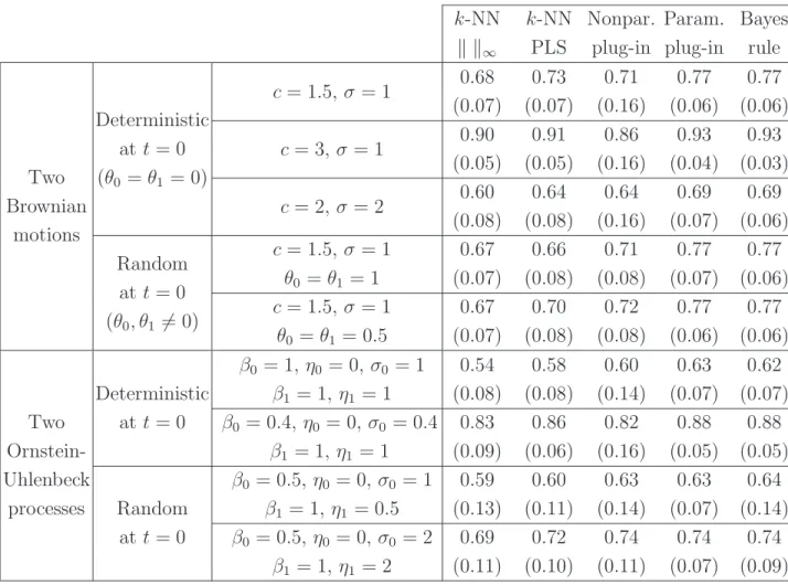
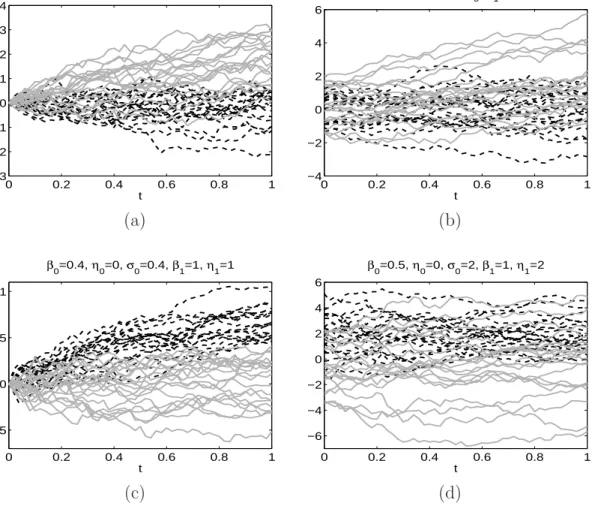
The observations will be realizations of two Ornstein-Uhlenbeck processes and two Brow-nian motions as described in Subsection 2.3. The parameters chosen for the pairs of processes are specified in Table 1 (in Figure 1 we have depicted some trajectories of the
processes used in the simulations). Figure 1
here.
We assume that p = P{Y = 0}, the proportion of observations coming from P0,
is 1/2 and is known in advance. For each i = 0,1 we take a training sample with size ni = 100 and a test sample with size 50 from Pi. The processes are observed at
equidistant times of the interval [0,1], t0 = 0, t1, . . . , tN = 1, with N = 50. We denote
by ∆ = tj −tj−1 the internodal distance. The number of Monte Carlo runs is 1000.
In each run we use the training sample to construct four classifiers: k-NN with the supremum norm and with a PLS-based semimetric (see e.g. Ferraty and Vieu, 2006, p. 30), parametric and nonparametric plug-in as introduced in Subsections 2.3 and 2.4 respectively. The performance of these classifiers is assessed by the proportion of correctly classified observations in the test samples. We also compute this proportion for the Bayes rule associated to each model. The number k of neighbours and the number of PLS directions for projection are chosen via cross-validation from a maximum of 10 neighbours and 5 PLS directions respectively.
When applying the nonparametric plug-in method to the data functions evaluated on the whole interval [0,1] we observed a noticeable boundary effect near 0, especially in the estimation ofv and its derivatives. This made the nonparametric plug-in method perform poorly. In order to avoid this, the Radon-Nikodym derivative for the nonpara-metric plug-in rule has been evaluated on the trajectories restricted to the interval [hn,1],
where hn is the same (and unique) smoothing parameter used in the estimation of the
derivatives ofui and vi. The value of hn has been chosen among{2∆,4∆, . . . ,20∆} via
classifica-tion error with the usual leave-one-out device (every training observaclassifica-tion is classified, as if it were a new incoming observation, using the remaining data as a training sample).
In Table 1 we display the mean and the standard deviation (between parentheses) of the proportion of correct classifications over the 1000 Monte Carlo samples. We see that the parametric plug-in procedure is the one performing best: it is very near the optimum.
As it could be expected, the nonparametric plug-in behaves worse than the para-metric one. Its best performance corresponds to the random start cases ui(0) > 0 for i = 0,1. In these situations, it is the second better classifier. When ui(0) = 0, the
parametric plug-in is still the winner, the k-NN with PLS is the second and the k-NN with the supremum metric and the nonparametric plug-in perform similarly.
It is interesting to note that thek-NN classification method is always reliable (even with the supremum metric, although PLS semimetric yields better results). Thus one of the conclusions of the study is that, when classifying functional data, the k-NN
procedure is generally a safe choice, free of model assumptions. Table 1
here.
4.2
A real data set
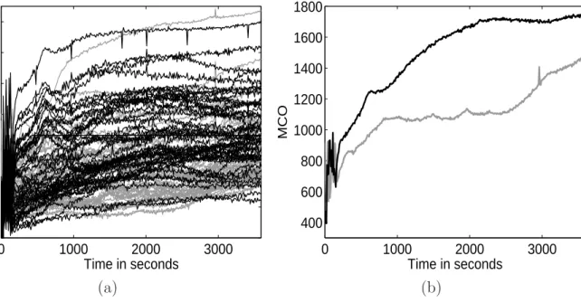
We compare the performance of the k-NN classification procedure with the nonpara-metric plug-in one in the analysis of data from research in experimental cardiology. The experiment was conducted at the Vall d’Hebron Hospital (Barcelona, Spain). See Ruiz-Meana et al. (2003) for biochemical and medical details on the data and Cuevas, Febrero and Fraiman (2004, 2006) for previous analysis of these observations.
The variable under study is the mitochondrial calcium overload (MCO), which mea-sures the level of the mitochondrial calcium ion (Ca2+). This variable was observed every 10 seconds during an hour in isolated mouse cardiac cells. The aim of the study was to assess whether a drug called Cariporide increased the MCO level. The data we analyze here consist of two samples of functions with sizes n0 = 45 (control group) and n1 = 44 (treatment group with Cariporide). In Figure 2 we display (a) all the data and
(b) the group means. Figure 2
here.
In many cases the first three minutes each curve shows oscillations which correspond to normal contractions of the cells. This first part of the curves has been eliminated (as in the original experiments with these data) because it has high variability and depends on uncontrolled factors.
To obtain a better approach of the distributions to normality, we have considered a transformation of the data, X = log(MCO−85). The performance of any of the clas-sification procedures considered is described by the probability of correctly classifying one of the transformed observations, approximated via cross-validation.
Obviously, in this case, we do not have enough information to consider using the parametric plug-in classifier. Consequently we only employ the k-NN (with uniform metric and PLS-based semimetric) and the nonparametric plug-in discrimination rules. The results appear in Table 2. It is interesting to notice that the results in this case, in some sense, are the opposite to those obtained with the simulations. The nonparametric plug-in clearly outperforms the other two and thek-NN with the supremum metric does
better than the k-NN with PLS. Table 2
here. Acknowledgement. The authors want to thank Javier Segura for bringing to our
knowledge some numerical differentiation techniques (in particular, the k-point rule).
5
Appendix
A.1 Parameter estimation for the models of Subsection 2.3 Two Brownian motions
In the simulations of Section 4 the estimator ofcis ˆc= arg mincPN
j=1( ˆm0(tj)−c tj)2,
where mi is the sample mean of the observations coming from Pi. The parameters θi and σ2 are respectively estimated by ˆθi = Pnj=1i (Xj(0;i)−mˆi(0))2/(ni −1) and
ˆ σ2 =P i=0,1 Pni j=1(Xj(1;i)−mˆi(1)−Xi(0;i) + ˆmi(0)) 2 /(n0+n1 −1). Two Ornstein-Uhlenbeck processes
The estimation of the unknown parameters (βi, ηi and σi, i = 0,1) is carried out
via linear least-squares regression between the realizations of the process at consecutive time points. The main idea is that, for i= 0,1 and for any 0 ≤s < t≤1, we have
X(t;i) = X(s;i)e−βi(t−s)+ η
i(1−e−βi(t−s)) +σi
p
1−e−2βi(t−s)Z, (25)
whereZ isN(0,1). The updating formula (25) is valid when X(0;i) is either determin-istic or random. In particular, fori= 0,1,k = 1, . . . , ni and j = 0, . . . , N −1,
Xk(tj+1;i) = aiXk(tj;i) +bi+σi
p
1−e−2βi∆Z
kj, (26)
whereai :=e−βi∆, bi :=ηi(1−e−βi∆) and Zkj are i.i.d. variables N(0,1).
Observe that, by estimating the parameters of the simple linear regression equation (26), we can construct estimators of βi, ηi and σi. When X(0;i) is deterministic, we
compute the least-squares estimators ofaiandbi, that is, the values ˆai and ˆbi minimizing
Pni
k=1
PN−1
j=0 u2kj, where ukj :=Xk(tj+1;i)−(ˆaiXk(tj;i) + ˆbi) are the residuals. Then
ˆ βi =− log(ˆai) ∆ , ηˆi = ˆbi 1−ˆai , σˆi2 = 1 (1−ˆa2 i)(niN −2) ni X k=1 N−1 X j=0 u2kj. (27)
When X(0;i) is random, we can compute ˆβi and ˆσ2i as in (27), but ηi is better
estimated by ˆηi =Pnj=1i PNk=0Xij(tk)/(ni(N + 1)).
A.2 Proofs of the results in 2.4 Proof of Proposition 1
(a) By the functional CLT in (C[0,1],k · k) (see p. 172 in Araujo and Gin´e, 1980) the sequence √n( ˆmn−m) converges weakly. This entails that the sequence k√n( ˆmn−m)k
is bounded in probability which in turn implies (16). Concerning (17) and (18), let us denoteX∗
i(t) =Xi(t)−m(t), t∈[0,1], i= 1,2, . . .. Note that, for t ∈[hn,1−hn],
|m′(t)−mˆ′n(t)| ≤ m′(t)− m(t+hn)−m(t−hn) 2hn + 1 2hnn n X i=1 Xi∗(t+hn) + 1 2hnn n X i=1 Xi∗(t−hn) ≤ m′(t)− m(t+hn)−m(t−hn) 2hn + 1 hnn n X i=1 Xi∗ . (28) The CLT applied to the sequence {X∗
n} allows us to conclude that the second term in
the right-hand side of (28) is OP (n1/2hn)−1
. A second order Taylor expansion of the first term implies that there exist ψn(1) ∈(t−hnt) and ψn(2) ∈(t, t+hn) such that
m′(t)−m(t+hn)−m(t−hn) 2hn = hn 4 m′′(ψn(1))−m′′(ψn(2)) ≤ Lh2 n 4 =O(h 2 n),
whereL is the Lipschitz constant associated with m′′.
Applying a similar reasoning to (18), we obtain that, ift ∈[hn,1−hn], then,
|m′′(t)−mˆ′′n(t)| ≤ m′′(t)− m(t+hn) +m(t−hn)−2m(t) h2 n + 4 1 h2 nn n X i=1 Yi . (29) The CLT implies that the order of the second term in (29) is OP (n1/2h2n)−1
. A second order Taylor’s expansion on t again gives that
m′′(t)−m(t+hn) +m(t−hn)−2m(t) h2 n = m′′(t)−1 2 m ′′(ψ(1) n ) +m′′(ψ(2)n ) ≤ Lhn. (b) Since ˆ Γ(t,1)−Γ(t,1) = 1 n X i (Xi∗(t) +m(t)−mˆn(t))(Xi∗(1) +m(1)−mˆn(1)) ! −Γ(t,1) = 1 n X i Xi∗(t)Xi∗(1)−Γ(t,1) ! + (m(t)−mˆn(t)) 1 n X i Xi∗(1) +(m(1)−mˆn(1)) 1 n X i Xi∗(t) + (m(t)−mˆn(t))(m(1)−mˆn(1)),
then kΓ(ˆ ·,1)−Γ(·,1)k ≤ 1 n X i (Xi∗Xi∗(1)−Γ(·,1)) +km−mˆnk 1 n X i Xi∗(1) +|m(1)−mˆn(1)| 1 n X i Xi∗ +km−mˆnk |m(1)−mˆn(1)| =: Tn(1)+Tn(2)+Tn(3)+Tn(4).
The assumption EkX1k4 < ∞ implies EkXi∗Xi∗(1)k2 < ∞ and thus the sequence
{X∗
iXi∗(1)}satisfies the CLT in the supremum norm. Then, sinceE[Xi∗Xi∗(1)] = Γ(·,1),
we have that Tn(1) = OP(n−1/2). Also Tn(2) = OP(n−1) because the CLT (real case)
im-plies that P
iXi∗(1)/n = OP(n−1/2) and, according to Proposition 1 (a), km−mˆnk = OP(n−1/2).
The CLT applied to{X∗
i}and Proposition 1 (a) yield thatT (3)
n andTn(4) areOP(n−1).
This allows us to conclude (19). The derivatives of Γ(·,1) are handled as those of m. The estimators of Γ(0,·) andσ(·) behave analogously to Γ(·,1). ✷
Proof of Proposition 2
a)According to expression (22) for ˆvn(t), this estimator is a quotient of two convergent
sequences. As that in the denominator, ˆun(0), converges to u(0) > 0, an upper bound
for the overall rate of the quotient is the slowest rate between ˆΓn(0, t) and ˆun(0). Similar
arguments apply for the first and second derivatives.
b) Let t ∈ [δn,1]. The hypothesis on u′ implies that inft≥δnu(t) ≥ O(δn). Since
n−1/2 = o(δ
n), from (19) we obtain that inft≥δnuˆn(t) ≥ OP(δn). Therefore, a direct
calculation based on the expression of ˆvn together with Proposition 1 b) leads to
sup t∈[δn,1] |vˆn(t)−v(t)|=OP 1 δn√n . (30)
The same reasoning, taking into account the relative orders betweenδn and hn leads to
sup t∈[δn,1] |ˆvn′(t)−v′(t)| = OP 1 δnhn√n +O h2 n δn (31) sup t∈[δn,1] |vˆ′′n(t)−v′′(t)| = OP 1 δnh2n√n +O hn δ2 n . (32)
with the definition (23) of ˆvn, we obtain that there exists ψn∈(t, δn) such that |ˆvn(t)−v(t)| ≤ |ˆvn(δn)−v(δn)|+ (δn−t)|vˆn′(δn)−v′(δn)| +1 2(t−δn) 2 |vˆn′′(δn)−v′′(δn)|+ 1 2(t−δn) 2 |v′′(δn)−v′′(ψn)| ≤OP 1 δn√n +OP 1 hn√n +O h2 n +OP δn h2 n √ n +O(hn) +O(δ3n) =OP δn h2 n √ n +O(hn) +O(δn3),
where we have applied (30), (31) and (32) and the fact that v′′ is Lipschitz. Then the first statement in Proposition 2 b) is deduced from here and (30). The remaining two
statements are proved similarly. ✷
Next we state a technical lemma which will be employed to prove Theorem 3.
Lemma 1 Let {Y(t), t ∈[0,1]} be a stochastic process whose mean function m(t) and variance functionσ2(t)satisfy thatm(0) =σ(0) = 0and both have a bounded derivative. Let {δn} be positive numbers which converge to zero. Then
E Z δn 0 | Y(t)|dt=O(δn3/2) and E Z δn 0 Y2(t)dt=O(δ2n).
Proof: Let H be a common upper bound for the derivatives ofm2 and σ2.
Z δn 0 E| Y(t)|dt ≤ Z δn 0 E 1/2(Y2(t))dt= Z δn 0 (m(t)2+σ2(t))1/2dt ≤ (2H)1/2 Z δn 0 t1/2dt=O(δn3/2).
The second statement in the lemma follows analogously. ✷
Proof of Theorem 3: From expressions (8) and (9) we see that f = dµ0/dµ1 is a
function of mi, ui, vi and their derivatives. Statement a) corresponds to the simplest
case in which ui(0) >0. In this situation, the simple structure of the estimators shows
that an upper bound for the convergence rate for logfn(x) is the worst rate for the
estimators involved in its definition, namely that of the estimators v′′
0 and v1′′.
Hence, we concentrate on part b). For simplicity we will omit the sub-index invi for
the rest of the proof. First notice that in the expressions fordµ0/dµ1 which we obtained
in Theorem 2 the second derivatives of v only appear inside integrals. In other words, we only need to care about differences of the type
Z 1 0 Xr(t)(ˆkn(t)ˆvn′′(t)−k(t)v′′(t))dt=OP Z 1 0 Xr(t)k(t)(ˆvn′′(t)−v′′(t))dt , (33)
forr = 1,2. Here k is a function depending on u, v, u′, v′, m and m′ and X is a mixture of the Brownian motions under consideration. Let us analyze the case in Theorem 2 b) for which r = 1 and the function k can be expressed as k =k1/(v((vu′−uv′)2), where k1 is a function which can be written in terms of u, v, u′, v′, m and m′. Therefore, the
assumptions in Theorem 2, imply that k is bounded. LetK be an upper bound of k. We split in two the integral in the right-hand side of (33), over the intervals [0, δn]
and [δn,1]. Now, from (32) in the proof of Proposition 2, we have that
E | Z 1 δn X(t)k(t)(ˆv′′ n(t)−v′′(t))dt| X1, . . . , Xn ≤ OP 1 δnh2n √ n +O hn δ2 n Z 1 δn E(X2(t))dt 1/2 . (34)
With respect to the other integral, we have that
E | Z δn 0 X(t)k(t)(ˆvn′′(t)−v′′(t))dt| X1, . . . , Xn ≤Kkvˆn′′−v′′k E Z δn 0 | X(t)|dt=OP δn1/2 √ n ! +O hn δn1/2 +O(δn5/2), (35)
where the last equality comes from Lemma 1 and Proposition 2 b). Equations (34) and (35) give E | Z 1 0 X(t)k(t)(ˆv′′n(t)−v′′(t))dt| X1, . . . , Xn ≤OP 1 δnh2n √ n +O hn δ2 n +O(δ5/2n ).
Takinghn =δn9/2 and δn =n−1/25 equates the three terms and yields the result. ✷
Proof of Proposition 3: It follows the same steps as the proof of Proposition 1, the
only difference being that if we apply a third order Taylor expansion in (29), we obtain
m′′(t)− m(t+hn) +m(t−hn)−2m(t) h2 n = hn 3! m′′′(ψn1)−m′′′(ψn2) ≤ Lh2 n 3! ,
and the result follows. ✷
Proof of Theorem 4: Let us use the following inequality (see, e.g., Devroye et al.,
1996, p. 93)
ˆ
Ln−L∗ ≤2E(|η(X)−ηn(X)| | Xn),
whereηis given in (5) andηnis obtained substitutingf =dµ0/dµ1by ˆfnin (5). Without
Observe that,f and ˆfnare always positive since they are Radon-Nikodym derivatives
of one probability measure with respect to another. Thus, for any x, we have
|η(x)−ηn(x)|= |
f(x)−fˆn(x)|
(1 + ˆfn(x)(1 +f(x))
≤ |f(x)−fˆn(x)|,
which implies that
ˆ Ln−L∗ ≤2E |f(x)−fˆn(x)| Xn . (36)
We obtain convergence rates (in probability) for the conditional expectation in the right of (36). Since all the cases are similar, let us consider the simple situation in which
m0 6=m1 and Γ0 = Γ1 = Γ with Γ(s, t) =u(min(s, t))v(max(s, t)). Then f −fˆn= dPm0,Γ dPm1,Γ − dPm0,ˆ ˆΓ0 dPmˆ1,ˆΓ1 = dPm0,Γ dPm1,Γ − dPm0,ˆ ˆΓ0 dPmˆ1,ˆΓ0 + dPm0ˆ ,Γ0ˆ dPmˆ1,Γˆ0 1− dPm1,ˆ Γ0ˆ dPmˆ1,Γˆ1 ! . (37) By Theorem 2 (b) and the mean value theorem we have that, for any x,
dPm0,Γ dPm1,Γ
(x)−dPm0,ˆ Γ0ˆ
dPmˆ1,Γˆ0
(x) =ez(z1−z2),
where (using the notation of Theorem 2)
z1 = D1+ D2−2 G(0) v(0) x(0) + 2G(1) v(1) x(1)−2 Z 1 0 x(t) v(t)G ′(t)dt, z2 = Dˆ1;0+ Dˆ2;0−2 ˆ G(0) ˆ v0(0) ! x(0) + 2Gˆ0(1) ˆ v0(1) x(1)−2 Z 1 0 x(t) ˆ v0(t) ˆ G′0(t)dt
and z = λ z1 + (1−λ)z2 for some λ ∈ [0,1]. The subscripts 0 in the expression of z2
mean that the estimation is carried out only with the sample from P0.
Consequently, E |dPm0,Γ dPm1,Γ (X)− dPmˆ0,ˆΓ0 dPm1,ˆ ˆΓ0 (X)| Xn ! ≤E ( e|Z1|+|Z2| " |D1−Dˆ1;0|+ |D2−Dˆ2;0|+ 2 G(0) v(0) − ˆ G(0) ˆ v0(0) ! |X(0)| +2 G(1) v(1) − ˆ G0(1) ˆ v0(1) |X(1)|+ 2 Z 1 0 | X(t)| G′(t) v(t) − ˆ G′ 0(t) ˆ v0(t) dt # Xn ) (38) ≤κ ( |D1−Dˆ1;0|E eAkXk|Xn + |D2−Dˆ2;0|+ 2 max t=0,1 G(t) v(t) − ˆ G0(t) ˆ v0(t) (39) +2 Z 1 0 G′(t) v(t) − ˆ G′ 0(t) ˆ v0(t) dt ! E kXkeAkXk|Xn ) (40)
whereκ = exp(|D1|+|Dˆ1;0|) and A= max |D2|+|Dˆ2;0|, G v + ˆ G0 ˆ v0 , G′ v + ˆ G′ 0 ˆ v0 ! .
Using Propositions 1 and 2 we obtain that the conditional expectations appearing in (39) and (40) are bounded in probability. Then
E |dPdPm0,Γ m1,Γ (X)−dPm0,ˆ ˆΓ0 dPmˆ1,ˆΓ0 (X)| Xn ! =OP max j=1,2|Dj − ˆ Dj;0| +OP max t=0,1 G(t) v(t) − ˆ G0(t) ˆ v0(t) ! +OP Z 1 0 G′(t) v′(t) − ˆ G′ 0(t) ˆ v′ 0(t) dt ! .
To find the convergence rates to 0 of these last three terms we use the expressions of D1, D2 and G appearing in Theorem 2. Some straighforward computations yield
|D1−Dˆ1;0|=OP(kvˆ0′ −v′k), |D2−Dˆ2;0|=OP(kvˆ0−vk), max t=0,1 G(t) v(t) − ˆ G0(t) ˆ v0(t) =OP(kˆv0′ −v′k) and Z 1 0 G′(t) v′(t) − ˆ G′ 0(t) ˆ v′ 0(t) dt=OP(kˆv0′′−v′′k). Thus we get E |dPdPm0,Γ m1,Γ (X)− dPm0ˆ ,Γ0ˆ dPm1ˆ ,Γ0ˆ (X)| Xn ! =OP(kvˆ0′′−v′′k). (41)
Let us now focus on the last term of (37). The analysis is similar to the one carried out above. On the one hand, for any x it holds that
dPm0,ˆ ˆΓ0 dPm1,ˆ ˆΓ0
(x)≤κ e2Bkxk,
where B = max(|Dˆ2;0|,kGˆ0/ˆv0k,kGˆ′0/ˆv0k). On the other hand, for any x it also holds
that 1−dPm1,ˆ Γ0ˆ dPmˆ1,Γˆ1 (x) ≤ |C1−Cˆ1|+ 1 2Cˆ1e Λkxk2 |Cˆ3|x2(0) +|Cˆ2|x2(1) + Z 1 0 x2(t) |Fˆ ′(t)| ˆ v0(t)ˆv1(t) dt ! (42) ≤ |C1−Cˆ1|+ ˆC1ΛeΛkxk 2 kxk2, where Λ = (|Cˆ3|+|Cˆ2|+ R1 0 |Fˆ ′|/(ˆv 0ˆv1))/2. Consequently E dPm0,ˆ Γ0ˆ dPm1,ˆ Γ0ˆ (X)|1−dPm1,ˆ Γ0ˆ dPm1,ˆ Γ1ˆ (X)| Xn ! ≤κn|C1−Cˆ1|E e2BkXk|Xn + ˆC1ΛE kXk2e2BkXk+ΛkXk2 Xn o . (43)
The conditional expectations in (43) and ˆC1areOP(1). The term Λ isOP(maxj=0,1kvˆ′′j− v′′k). The difference |C
1 −Cˆ1| is OP(maxj=0,1kˆvj − vk). Thus the term in (43) is OP(maxj=0,1kvˆj′′−v′′k). This, together with (41) and Proposition 2 (a), yield the desired
result. ✷
References
Abraham, C., Biau, G. and Cadre, B. (2006). On the kernel rule for function classifica-tion. Ann. Inst. Stat. Math. 58, 619–633.
Araujo A. and Gin´e, E. (1980). The Central Limit Theorem for Real and Banach Valued Random Variables. Wiley.
Audibert, J.Y. and Tsybakov, A.B. (2007). Fast learning rates for plug-in classifiers.
Ann. Statist. 35, 608–633.
Ba´ıllo, A., Cuevas, A. and Fraiman, R. (2009). Classification methods for functional data. To appear in Oxford Handbook on Statistics and FDA, F. Ferraty and Y. Romain, eds. Oxford University Press.
C´erou, F. and Guyader, A. (2006). Nearest neighbor classification in infinite dimension.
ESAIM Probab. Stat. 10, 340-355.
Cuevas, A., Febrero, M. and Fraiman, R. (2004). An anova test for functional data.
Comput. Statist. Data Anal. 47, 111–122.
Cuevas, A., Febrero, M. and Fraiman, R. (2006). On the use of the bootstrap for estimating functions with functional data. Comput. Statist. Data Anal. 51, 1063– 1074.
Devroye, L., Gy¨orfi, L. and Lugosi, G. (1996). A Probabilistic Theory of Pattern Recog-nition. Springer, New York.
Duda, R.O., Hart, P.E., Stork, D.G. (2000). Pattern Classification, 2nd edition. Wiley. Ferraty, F. and Vieu, P. (2006). Nonparametric Functional Data Analysis: Theory and
Practice. Springer.
Feldman, J. (1958). Equivalence and perpendicularity of Gaussian processes. Pacific J. Math. 8, 699–708.
Fisher, R.A. (1936). The use of multiple measurements in taxonomic problems. Annals of Eugenics7, 179–188.
Folland, G. B. (1999). Real Analysis Modern Techniques and their Applications. Wiley, New York.
Gautschi, W. (1997). Numerical Analysis. An Introduction. Birkh¨auser. Boston. Hand, D. (2006). Classifier technology and the illusion of progress. Statist. Sci. 21,
Hastie, T., Tibshirani, R. and Friedman, J. (2001). The Elements of Statistical Learning.
Springer. New York.
Herzeg, D. and Cvetkovic, L. (1986). On a numerical differentiation. SIAM J. Numer. Anal. 23, 686–691.
James, G. M., Hastie, T. J. (2001). Functional linear discriminant analysis for irregularly sampled curves. J. Roy. Statist. Soc. Ser. B63, 533–550.
Jørsboe, O. G. (1968). Equivalence or Singularity of Gaussian Measures on Function Spaces. Various Publications Series, No. 4, Matematisk Institut, Aarhus Universitet, Aarhus.
Ramsay, J.O. and Silverman, B.W. (2005). Functional Data Analysis. Second edition. Springer.
Ruiz-Meana, M., Garc´ıa-Dorado, D., Pina, P., Inserte, J., Agull´o, L. and Soler-Soler, J. (2003). Cariporide preserves mitochondrial proton gradient and delays ATP depletion in cardiomyocites during ischemic conditions. Am. J. Physiol. Heart Circ. Physiol. 285, H999-H1006.
Sacks, J. and Ylvisaker, N.D. (1966). Designs for regression problems with correlated errors. Ann. Math. Statist. 37, 66–89.
Segall, A. and Kailath, T. (1975). Radon-Nikodym derivatives with respect to measures induced by discontinuous independent-increment processes. Ann. Probab. 3, 449– 464.
Shin, J. (2008). An extension of Fisher’s discriminant analysis for stochastic processes.
J. Multiv. Anal. 99, 1191–1216.
Stone, C. J. (1977). Consistent nonparametric regression. Ann. Statist. 5, 595–645. Vakhania, N.N. (1975). The topological support of Gaussian measure in Banach space.
Nagoya Math. J. 57, 59–63.
Varberg, D.E. (1961). On equivalence of Gaussian measures. Pacific J. Math. 11, 751–762.
Varberg, D.E. (1964). On Gaussian measures equivalent to Wiener measure. Trans. Amer. Math. Soc. 113, 262–273.
k-NN k k∞ k-NN PLS Nonpar. plug-in Param. plug-in Bayes rule Two Brownian motions Deterministic att = 0 (θ0 =θ1 = 0) c= 1.5,σ = 1 0.68 0.73 0.71 0.77 0.77 (0.07) (0.07) (0.16) (0.06) (0.06) c= 3, σ = 1 0.90 0.91 0.86 0.93 0.93 (0.05) (0.05) (0.16) (0.04) (0.03) c= 2, σ = 2 0.60 0.64 0.64 0.69 0.69 (0.08) (0.08) (0.16) (0.07) (0.06) Random att = 0 (θ0, θ1 6= 0) c= 1.5,σ = 1 θ0 =θ1 = 1 0.67 0.66 0.71 0.77 0.77 (0.07) (0.08) (0.08) (0.07) (0.06) c= 1.5,σ = 1 θ0 =θ1 = 0.5 0.67 0.70 0.72 0.77 0.77 (0.07) (0.08) (0.08) (0.06) (0.06) Two Ornstein-Uhlenbeck processes Deterministic att = 0 β0 = 1, η0 = 0, σ0 = 1 β1 = 1, η1 = 1 0.54 0.58 0.60 0.63 0.62 (0.08) (0.08) (0.14) (0.07) (0.07) β0 = 0.4,η0 = 0, σ0 = 0.4 β1 = 1, η1 = 1 0.83 0.86 0.82 0.88 0.88 (0.09) (0.06) (0.16) (0.05) (0.05) Random att = 0 β0 = 0.5,η0 = 0, σ0 = 1 β1 = 1, η1 = 0.5 0.59 0.60 0.63 0.63 0.64 (0.13) (0.11) (0.14) (0.07) (0.14) β0 = 0.5,η0 = 0, σ0 = 2 β1 = 1, η1 = 2 0.69 0.72 0.74 0.74 0.74 (0.11) (0.10) (0.11) (0.07) (0.09) Table 1: Results of the Monte Carlo study
k-NN k k∞ k-NN PLS Nonpar. plug-in 0.79 0.66 0.85
0 0.2 0.4 0.6 0.8 1 −3 −2 −1 0 1 2 3 4 t c=1.5, σ=1 0 0.2 0.4 0.6 0.8 1 −4 −2 0 2 4 6 t c=1.5, σ=1, θ 0=θ1=1 (a) (b) 0 0.2 0.4 0.6 0.8 1 −0.5 0 0.5 1 t β0=0.4, η0=0, σ0=0.4, β1=1, η1=1 0 0.2 0.4 0.6 0.8 1 −6 −4 −2 0 2 4 6 t β0=0.5, η0=0, σ0=2, β1=1, η1=2 (c) (d)
Figure 1: Some trajectories (P0 in gray andP1 in dotted black) of the processes used in
the Monte Carlo study. In (a) and (b) we have two Brownian motions and in (c) and (d) the processes are Ornstein-Uhlenbeck. In (a) and (c) X(0)|Y =iis 0 and in (b) and (d) it is random.
0 1000 2000 3000 0 500 1000 1500 2000 2500 3000 3500 Time in seconds MCO 0 1000 2000 3000 400 600 800 1000 1200 1400 1600 1800 Time in seconds MCO (a) (b)
Figure 2: Cell data (control group in grey and treatment group in black): (a) all the original observations; (b) sample means.