GF-CLUST: A nature-inspired algorithm for automatic text clustering

(1)

57

GF-CLUST: A NATURE-INSPIRED ALGORITHM FOR AUTOMATIC TEXT CLUSTERING

1_{Athraa Jasim Mohammed,}2_{Yuhanis Yusof &} 2_{Husniza Husni}

1_{University of Technology, Baghdad, Iraq}

2_{Universiti Utara Malaysia, Malaysia}

[email protected]; [email protected]; [email protected]

ABSTRACT

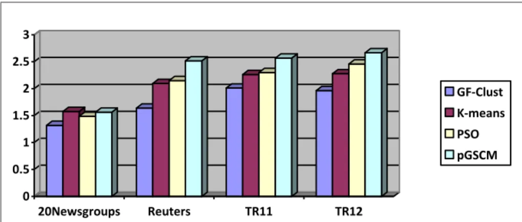
Text clustering is a task of grouping similar documents into a cluster while assigning the dissimilar ones in other clusters. A well-known clustering method which is the K-means algorithm is extensively employed in many disciplines. However, there is a big challenge to determine the number of clusters using K-means. This paper presents a new clustering algorithm, termed Gravity Firefly Clustering (GF-CLUST) that utilizes Firefly Algorithm for dynamic document clustering. The GF-CLUST features the ability of identifying the appropriate number of clusters for a given text collection, which is a challenging problem in document clustering. It determines documents having strong force as centers and creates clusters based on cosine similarity measurement. This is followed by selecting potential clusters and merging small clusters to them. Experiments on various document datasets, such as 20Newgroups, Reuters-21578 and TREC collection are conducted to evaluate the performance of the proposed GF-CLUST. The results of purity, F-measure and Entropy of GF-CLUST outperform the ones produced by existing clustering techniques, such as K-means, Particle Swarm Optimization (PSO) and Practical General Stochastic Clustering Method (pGSCM). Furthermore, the number of obtained clusters in GF-CLUST is near to the actual number of clusters as compared to pGSCM.

Keywords: Firefly algorithm, text clustering, divisive clustering, dynamic clustering.

(2)

58

INTRODUCTION

Text documents, such as articles, blogs and news, are periodically increased in the Web. This increase has made online users to require more time and effort to obtain relevant information. In this context, manual analysis and manual discovery of beneficial information are very difficult. Hence, it is relevant to provide automatic tools for analysing large textual collections. Referring to such needs, data mining tasks, such as classification, association analysis and clustering are commonly integrated in the tools.

Clustering is a technique of grouping similar documents into a cluster and dissimilar documents in a different cluster (Aggarwal, & Reddy, 2014). It is a descriptive task of data mining where the algorithm learns by identifying similarities between items in a collection. According to Gil-Garicia and Pons-Porrata (2010), clustering algorithms are classified into two categories based on prior information (i.e., number of clusters): static and dynamic. In static clustering, a set of objects is classified into a determined number of clusters, while in the dynamic clustering, the objects are automatically grouped based on some criteria to discover the right number of clusters.

Clustering can also be carried out in two ways: soft clustering or hard clustering (Aliguliyev, 2009). In soft clustering, each object is grouped to be a member of any or all clusters with different membership grades, while in the case of hard clustering, the objects are members of a single cluster. Based on the mechanics of constructing the clusters, clustering methods can be divided into two categories: Hierarchical clustering and Partitional clustering (Forsati, Mahdavi, Shamsfard, & Meybodi, 2013; Luo, Li, & Chung, 2009). Hierarchical clustering methods create a tree of clusters, while Partitional clustering methods create a flat of clusters (Forsati, Mahdavi, Shamsfard, & Meybodi, 2013). This study focuses on dynamic, hard and hierarchical clustering.

LITERATURE REVIEW

Previous studies divided clustering algorithms into two main categories: Hierarchical and Partitional (Forsati et al., 2013; Luo et al., 2009). The Hierarchical clustering methods create a hierarchy of clusters (Forsati, Mahdavi, Shamsfard, & Meybodi, 2013). It is an efficient method for document clustering in information retrieval as it provides data-view at different levels and organizes the document collection in a structured manner. Based on the mechanics of constructing a hierarchy, it has two approaches:

(3)

59

Agglomerative and Divisive hierarchical clustering. The Agglomerative clustering approach operates from bottom to top, where every document is assumed as a single cluster. The approach attempts to merge any closest clusters based on dissimilarity matrix. There are three methods that are used for merging: single linkage, complete linkage and average linkage or also known as UPGMA (un-weighted pair group method with arithmetic mean). Details on these methods can be found in previous work, such as Yujian and Liye (2010). On the other hand, divisive clustering builds a tree of multi-level clusters (Forsati, Mahdavi, Shamsfard, & Meybodi, 2013). All objects are initially in a single cluster and at each level, the clusters are split into two clusters. Such an operation is demonstrated in Bisect K-means (Kashef, & Kamel, 2010, 2009). In the splitting process, it employs one of the partitional clustering algorithms that uses an objective function. This objective function has the ability to minimize the distance between a center and objects in one cluster and maximizes the distance between clusters.

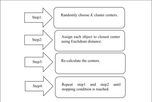
A well-known example of a hard and static partitional clustering is the K-means (Jain, 2010). It initially determines a number of clusters and then assigns objects of a collection into the predefined clusters while trying to minimize the sum of squared error over all clusters. This process continues until a specific number of iterations is achieved. Figure 1 illustrates the steps involved in K-means. The K-means algorithm is easy to implement and efficient. However, it suffers from some drawbacks: random initialization of centers (including the determination of number of clusters) may cause the solution to be trapped into local optima. To overcome such weakness, a research area that employs meta-heuristics has been developed. It optimizes the solution to search for global optimal or near optimal solution using an objective function (Tang, Fong, Yang, & Deb, 2012). Problems are formulated as either a minimum or maximum function (Rothlauf, 2011).

There are two types of Meta-heuristic approaches: single meta-heuristic solution and population meta-heuristic solution (Boussaïd, Lepagnot, & Siarry, 2013). Single meta-heuristic solution initializes one solution and moves away from it, such as implemented in the Simulated Annealing (Kirkpatrick, Gelatt, & Vecchi, 1983) and Tabu Search (Glover, 1986). Population meta-heuristic solution initializes multi solutions and chooses the best solution based on evaluation of solutions at each iteration, such as in Genetic algorithm (Beasley, Bull, & Martin, 1993), Evolutionary programming (Fogel, 1994), Differential Evolution (Aliguliyev, 2009) and nature-inspired algorithms (Bonabeau, Dorigo, & Theraulaz, 1999). The nature-inspired algorithm, also known as Swarm intelligence, is related to the collective behavior of social insects or animals in solving hard problems (Rothlauf, 2011). Swarm intelligence,

(4)

60

includes Particle Swarm Optimization (PSO) (Kennedy, & Eberhart, 1995), Artificial Bee Colony (Mahmuddin, 2008; Mustaffa, Yusof, & Kamaruddin, 2013), and Firefly Algorithm (Yang, 2010).

Figure 1. Steps of K-means (Jain, 2010).

With regards to the population meta-heuristic approach, Aliguliyev (2009) developed a modified differential evolution (DE) algorithm for text clustering that optimized various density based criterion functions: internal, external and hybrid functions. The result indicates that the proposed DE algorithm speeds up the convergence. On the other hand, the PSO, proposed by Kennedy and Eberhart (1995) was used for document clustering in Cui, Potok, & Palathingal (2005). The basic idea of PSO comes from the flock and foraging behavior where each solution has n dimensions search space. The birds do not have search space, so it is called “Particles”. Each particle has a fitness function value that can be computed using a velocity of particles flight direction and distance. The basic PSO clustering algorithm (Cui, Potok, & Palathingal, 2005) is illustrated in Figure 2.

Initially, each particle randomly chooses a number of cluster centers from a vector of document dataset. Then, each particle performs three steps: creating clusters, evaluating clusters and creating new solutions. Creating clusters is done by assigning documents to the closest center. Evaluating clusters is done by evaluating the created clusters using fitness function (i.e., average distance

4

optimal solution using an objective function (Tang, Fong, Yang, & Deb, 2012). Problems are formulated as either a minimum or maximum function (Rothlauf, 2011).

Figure 1. Steps of K-means (Jain, 2010).

There are two types of Meta-heuristic approaches: single heuristic solution and population meta-heuristic solution (Boussaïd, Lepagnot, & Siarry, 2013). Single meta-heuristic solution initializes one solution and moves away from it, such as implemented in the Simulated Annealing (Kirkpatrick, Gelatt, & Vecchi, 1983) and Tabu Search (Glover, 1986). Population meta-heuristic solution initializes multi solutions and chooses the best solution based on evaluation of solutions at each iteration, such as in Genetic algorithm (Beasley, Bull, & Martin, 1993), Evolutionary programming (Fogel, 1994), Differential Evolution (Aliguliyev, 2009) and nature-inspired algorithms (Bonabeau, Dorigo, & Theraulaz, 1999). The nature-inspired algorithm, also known as Swarm intelligence, is related to the collective behavior of social insects or animals in solving hard problems (Rothlauf, 2011). Swarm intelligence, includes Particle Swarm Optimization (PSO) (Kennedy and Eberhart, 1995), Artificial Bee Colony (Mahmuddin, 2008; Mustaffa, Yusof, & Kamaruddin, 2013), and Firefly Algorithm (Yang, 2010).

Randomly choose K cluster centers. Step1:

Step2: Assign each object to closest center _{using Euclidean distance.}

Step3: Re-calculate the centers.

Step4: Repeat step1 and step2 until

stopping condition is reached.

(5)

61

between documents and center (ADDC)) and selecting the best solution from multiple solutions. The last step is creating new solutions which is done by updating the velocity and position of particle. The previous three steps are repeated until one of the stopping conditions is reached; the maximum number of iterations or the average change in center is less than a threshold (predefined value).

Figure 2. Steps in standard PSO clustering (Cui, Potok, & Palathingal, 2005).

Further work in clustering also includes Rashedi, Nezamabadi-pour and Saryazdi (2009) who proposed optimization algorithm that utilizew law of gravity and law of motion known as Gravitation Search Algorithm (GSA). They considered each agent as an object and determined their performance by their masses. The agents move towards heavier masses (the mass is calculated by map of fitness). The heavy masses represent good solutions. Later (Hatamlou, Abdullah, & Nezamabadi-pour, 2012), a hybrid Gravitational Search Algorithm with K-means (GSA-KM) for numerical data clustering was presented. GSA algorithm prevents K-means from trapping into local optima whereas the K-means algorithm speeds up the convergence of GSA. On the other hand, Fuzzy C-means (FCM) algorithm (which is a type of soft clustering) based on gravity and cluster merging is presented in Zhong, Liu, & Li (2010). It tries to find initial centers of clusters and solve the outlier’s sensitivity problem. It also utilizes the law of gravity but the calculation of mass is different where the mass of object p is the number of neighbourhood objects of p.

Each particle, randomly choose K cluster centers. Step1:

Step2:

For each Particle:

- Assign each document to closest center. - Compute the fitness value based on average

distance between documents and center (ADDC).

- Update the velocity and position of particle.

Step3: Repeat step2 until one of stop conditions is reached; the maximum number of iterations or the average change in center is less than threshold (predefined value).

(6)

62

Previous clustering algorithms (Cui, Potok, & Palathingal, 2005; Jain, 2010; Zhong, Liu, & Li, 2010) are denoted as static method which initially requires a pre-defined number of clusters. Hence, such algorithms are not appropriate to cluster data collections that are not accompanied with relevant information (i.e., number of classes or clusters). To date, such issues are solved using two approaches: estimation or by using dynamic swarm based approach. The first approach employs the validity index in clustering, which can drive to select the optimal number of clusters. Initially, it starts by determining a range of clusters (minimum and maximum number of clusters). Then, it performs clustering with the various numbers of clusters and chooses the number of clusters that produces the best quality performance. In the work of Sayed, Hacid and Zighed (2009), the clustering is of hierarchical agglomerative with validity index (VI) where at each level of merging step, it calculates the index of two closest clusters before and after merging. If the VI improves after merging, then merging of the clusters is finalized. This process continues until it reaches optimal clustering solution. Similarly, Kuo and Zulvia (2013) proposed an automatic clustering method, known as Automatic Clustering using Particle Swarm Optimization (ACPSO). It is based on PSO where it identifies number of clusters along with the usage of K-means that adjusts the clustering centers. The ACPSO determines the appropriate number of clusters in the range of [2, Nmax] . The result shows that ACPSO produces better accuracy and consistency compared to Dynamic Clustering Particle Swarm Optimization and Genetic (DCPG) algorithm, Dynamic Clustering Genetic Algorithm (DCGA) and Dynamic Clustering Particle Swarm Optimization (DCPSO). In the work of Mahmuddin (2008), a modified K-means and bees’ algorithm are integrated to estimate the total number of clusters in a dataset. The aim of using bees’ algorithm is to identify as near as possible the right centroids, while K-means is utilized to identify the best cluster. From previous discussions, it is learnt that the estimation approach is suitable for a problem that requires little or no knowledge of it; however, there is difficulty to determine the range of clusters for each dataset (lower and upper bound of number of clusters).

On the other hand, the dynamic swarm based approach can automatically find the appropriate number of clusters in a given data collection, without any support. Hence, it offers a more convenient cluster analysis. Dynamic swarm based approach adapts the mechanism of a specific insect or animal that is found in nature and converts it to heuristics rules. Each swarm employs it like an agent that follows the heuristic rules to carry out the sorting and grouping of objects (Tan, 2012). In literature, there are examples of such an

(7)

63

approach in solving clustering problems, such as Flocking based approach (Cui, Gao, & Potok, 2006; Picarougne, Azzag, Venturini, & Guinot, 2007) and Ant based clustering (Tan, Ting, & Teng, 2011a, 2011b). The Flocking based approach relates to behavior of swarm intelligence (Bonabeau et al., 1999) where a group of flocks swarm move in 2D or 3D search space following the same rules of flocks; get close to similar agents or far away from dissimilar agents (Picarougne, Azzag, Venturini & Guinot, 2007). This approach is computationally expensive as it requires multiple distance computations. On the other hand, the Ant based approach deals with behavior of ants, where each ant can perform sorting and corpse cleaning. This approach works by distributing the data object randomly in the 2D grid (search space), then determining a specific number of ants (agents) that move randomly in this grid to pick up a data item if it does not hold any object (item) and drop the object (item) if it finds similar object. This process continues until it reaches a specific number of iterations (Deneubourg et al., 1991).

Tan, Ting and Teng (2011b) proposed practical General Stochastic Clustering Method (pGSCM) that is a simplification of the Ant based clustering approach. The pGSCM is used to cluster multivariate real world data. The pseudo code of pGSCM is illustrated in Figure 3. The input of pGSCM is a dataset, D, that contains n objects and the output is the number of clusters discovered by pGSCM method, without any prior knowledge. In the initialization of pGSCM, the dissimilarity threshold for n objects is estimated. Then, it creates n bins where each bin includes one object from dataset D. Through the working of pGSCM, it selects two objects randomly from a dataset; if the distance between these two objects is less than their dissimilarity threshold, then the level of support of the two objects is compared. If object i has less support than j, then the lesser one is moved to the greater one and vice versa. At the end of iterations, a number of small and large bins are created. The large bins are selected as output clusters while the small bins are reassigned to large bins (objects in small bins assigned to similar center in large bins). The selected large bins process is based on threshold of 50, n/20 (means the threshold is 5% of the size of dataset, n); this threshold is based on criterion used by Picarougne, Azzag, Venturini, and Guinot (2007). This method performs well compared to the state-of-the-art methods; however, randomly selecting two objects in each iteration may create other issues. There is a chance that in some iterations, the same objects are selected or some objects are not selected at all. Furthermore, the selection process initially requires large number of iterations to increase the probability of selecting different objects.

(8)

64

Figure 3. Pseudo code of pGSCM clustering algorithm (Tan, Ting, & Teng, 2011b).

Of late, a newly inspired meta-heuristic algorithm has appeared, known as Firefly Algorithm (FA). FA was developed and presented at Cambridge University by Xin-She Yang in 2008. Firefly algorithm is related to behavior of firefly insects that produce short and rhythmic flashes (flashing light), where, the rate of rhythmic flashes and amount of time brings two fireflies together. Further, the distance between two fireflies also affects the light, where the light becomes weaker and weaker when the distance increases. Xin-She Yang formulated this mechanism by associating the flashing light with objective function f(x). The value of x is represented by the position of the firefly, where every position has various values of flashing light. Based on the problem (maximization or minimization) that we want to solve, we can deal with the objective function. There is another factor in FA algorithm affected by the distance of two fireflies which is the attractiveness β. This factor is changed based on the distance of two fireflies; when two fireflies are attracted to each

9

Figure 3. Pseudo code of pGSCM clustering algorithm (Tan, Ting, and Teng, 2011b).

Of late, a newly inspired meta-heuristic algorithm has appeared, known as Firefly algorithm (FA). FA was developed and presented at Cambridge University by Xin-She Yang in 2008. Firefly algorithm is related to behavior of firefly insects that produce short and rhythmic flashes (flashing light), where, the rate of rhythmic flashes and amount of time brings two fireflies together. Further, the distance between two fireflies also affects the light, where the light becomes weaker and weaker when the distance increases. Xin-She Yang formulated this mechanism by associating the flashing light with objective function f(x). The value of x is represented by the position of the firefly, where every position has various values of flashing light. Based on the problem (maximization or minimization) that we want to solve, we can deal with the objective function. There is another factor in FA algorithm affected by the distance of two fireflies which is the attractiveness β. This factor is changed based on the distance of two fireflies; when two fireflies are attracted to each other, the highest light will attract

Input: dataset D of n objects. Step1:

Step2: Estimate the dissimilarity threshold for n _objects.

Step3: Initialize n bins by allocating each object in D to _{a bin.}

While iteration <= maxiteration - i= random select (D) - j= random select (D)

- if d(i,j) < min (Ti,Tj) {Ti,Tj is dissimilarity threshold}

- Store the comparison outcome in Vi and Vj. - If c(i) < c(j) move i to j.

- Else move j to i. - End if

- End while Step4:

Step5: Return all non-empty bins as a set of final.

(9)

65

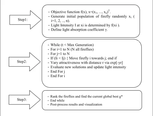
other, the highest light will attract the lower light; this process will cause the changing in the position of two fireflies and lead to change in the value of β. The pseudo code of standard Firefly Algorithm is illustrated in Figure 4.

Figure 4. Pseudo code of standard Firefly algorithm (Yang, 2010).

Firefly Algorithm (Yang, 2010) has been applied in many disciplines and proven to be successful in image segmentation (Hassanzadeh, Vojodi, & Moghadam, 2011) and dispatch problem (Apostolopoulos & Vlachos, 2011). Additionally, the Firefly Algorithm was utilized in numeric data clustering and proven successful. Senthilnath, Omkar, and Mani (2011) used Firefly algorithm in supervised clustering (the class for each object is defined) and also in static manner (the number of clusters is defined). In the process of this algorithm, each firefly at specific location x in 2D search space evaluated the fitness using objective function related to the sum of Euclidean distance on all training data. The result demonstrates that FA can be efficiently used for clustering. But Banati and Bajaj (2013) implemented the Firefly algorithm differently. They used FA as an unsupervised learning (the class for each object is undefined). However, their implementation is still based on static manner, as shown in Senthilnath, Omkar, and Mani’s (2011) work, where the number of clusters is pre-defined.

10

the lower light; this process will cause the changing in the position of two fireflies and lead to change in the value of β. The pseudo code of standard Firefly Algorithm is illustrated in Figure 4.

Figure 4. Pseudo code of standard Firefly Algorithm (Yang, 2010).

Firefly algorithm (Yang, 2010) has been applied in many disciplines and proven to be successful in image segmentation (Hassanzadeh, Vojodi, & Moghadam, 2011) and dispatch problem (Apostolopoulos & Vlachos, 2011). Additionally, the Firefly algorithm was utilized in numeric data clustering and proven successful. Senthilnath, Omkar, and Mani (2011) used Firefly algorithm in supervised clustering (the class for each object is defined) and also in static manner (the number of clusters is defined). In the process of this algorithm, each firefly at specific location x in 2D search space evaluated the fitness using objective function related to the sum of Euclidean distance on all training data. The result demonstrates that FA can be efficiently used for clustering. But Banati and Bajaj (2013) implemented the Firefly algorithm differently. They used FA as an unsupervised learning (the class for each object is undefined). However, their implementation is still based on static

- Objective function f(x), x=(x1, ..., xn)T_.

- Generate initial population of firefly randomly xi (

i=1, 2, .., n).

- Light Intensity I at xi is determined by f(xi ).

- Define light absorption coefficient γ.

Step1:

Step2:

Step3:

- While (t < Max Generation)

- For i=1 to N (N all fireflies)

- For j=1 to N

- If (Ii < Ij) { Move firefly i towards j; end if

- Vary attractiveness with distance r via exp[-yr]

- Evaluate new solutions and update light intensity

- End For j

- End For i

- Rank the fireflies and find the current global best g* - End while

- Post-process results and visualization

(10)

66

In this paper, Firefly Algorithm is proposed to cluster documents automatically using divisive clustering approach, and the algorithm is termed Gravity Firefly Clustering (GF-CLUST). The proposed GF-CLUST integrates the work on Gravitation Firefly Algorithm (GFA) (Mohammed, Yusof, & Husni, 2014a) with the criterion of selection clusters (Picarougne, Azzag, Venturini, & Guinot, 2007). GF-CLUST operates based on random positioning of documents that employs the law of gravity to find the force between documents which is used as the objective function.

METHODOLOGY

The proposed GF-CLUST works in three steps: data pre-processing, development of vector space model and data clustering, as shown in Figure 5. Data Pre-processing

This step is very important in any machine learning system. It can be defined as the process of converting a set of documents from unstructured into a structured form. This process involves three steps as shown in Figure 5: Data cleaning, stop word remover and word stemming. Initially, it starts by selecting texts from each document. The extracted texts are cleaned of special characters and digits. Then, the text undergoes a splitting process that divides each cleaned text into a set of words. Later, it removes words that have length less than three characters, such as in, on, at, etc., and removes stop words, such as propositions, conjunctions, etc. The last step in pre-processing is the stemming process, where all the words are retained as the root (Manning, Raghavan, & Schütze, 2008).

Development of Vector Space Model

This step is commonly used in information retrieval and data mining approach where it represents the utilized data in a vector space. In this work, each cleaned document is represented in 2D space (columns and rows). The column denotes terms, m, extracted from documents, while the rows refer to the documents, n. The term frequency-inverse document frequency (TF-IDF) is an efficient scheme that is used to identify significance of terms in the text, The benefit of utilizing TF-IDF is the balance between the local and global term weighting in a document (Aliguliyev, 2009; Manning, Raghavan, & Schutze, 2008). Equation 1 is used to calculate the TF-IDF.

tfidft,d tft,d*logN/dftt ₍₁₎ (1) R M M G F 2 2 1*  (2) Cdist d T d T d d y eSimilarit Co d d F( i* j) sin ( i* j) ( i)* ₂( j) (3)     m j i i j j i d d d d y eSimilarit Co 1 * ) ( ) * ( sin ₍₄₎    m i t d j tfidfi j d T 1 , ) ( ₍₅₎ 2 ₍ ₎2 ) * (Xi Xj Xi Xj Cdist   ₍₆₎      k j ni i K ni di ci Dis ADDC 1 1 ) * ( (7) 2 1 2 ) ( ) , (     m n jn in i j d d d d Dis ₍₈₎        k c j k N C P Purity ,.., 1 ) * ( (9) j k k j k C Max C P( * )   ₍₁₀₎ ) , ( * ) , ( ) , ( * ) , ( * 2 ( ,..., 1 max ) ( j C k P j C k R j C k P j C k R k C C j C k F            (11) k class of members the of number The j cluster in k class of members the of number The ) , ( _k C_j  R  ₍₁₂₎ j class of members the of number The j cluster in k class of members the of number The ) , ( _k C_j  P  ₍₁₃₎ j j k c k _j j k C C C C j HC       log ) ( 1 (14)    k j j j N C HC H 1 * (15)

http://jict.uum.edu.my

(11)

67 Data Clustering

This step includes two processes: identify centers and create clusters and selection of clusters. The identification of centers is achieved by using GFA (Mohammed, Yusof, & Husni, 2014a), where the GFA employs Newton’s law of gravity to determine the force between documents and uses it as an objective function. Newton’s law of gravity states that “Every point mass attracts every single other point mass by a force pointing along the line intersecting both points. The force is proportional to the product of the two masses and inversely proportional to the square of the distance between them” (Rashedi, Nezamabadi-pour, & Saryazdi, 2009). Equation 2 shows Newton’s law of gravity.

(2)

Figure 5. The process of Gravity Firefly clustering (GF-CLUST).

where F is the force between two masses, G is the gravitational constant, M₁

is the first mass, M₂ is the second mass, R is the distance between two masses.

t d t d t tf N dft tfidf,  , *log / ₍₁₎ R M M G F 2 2 1*  (2) Cdist d T d T d d y eSimilarit Co d d F( i* j) sin ( i* j) ( i)* ₂( j) ₍₃₎     m j i i j j i d d d d y eSimilarit Co 1 * ) ( ) * ( sin ₍₄₎    m i t d j tfidfi j d T 1 , ) ( ₍₅₎ 2 ₍ ₎2 ) * (Xi Xj Xi Xj Cdist   ₍₆₎      k j ni i K ni di ci Dis ADDC 1 1 ) * ( (7) 2 1 2 ) ( ) , (     m n jn in i j d d d d Dis ₍₈₎        k c j k N C P Purity ,.., 1 ) * ( (9) j k k j k C Max C P( * )   ₍₁₀₎ ) , ( * ) , ( ) , ( * ) , ( * 2 ( ,..., 1 max ) ( j C k P j C k R j C k P j C k R k C C j C k F            (11) k class of members the of number The j cluster in k class of members the of number The ) , ( _k C_j  R  ₍₁₂₎ j class of members the of number The j cluster in k class of members the of number The ) , ( _k C_j  P  ₍₁₃₎ j j k c k _j j k C C C C j HC       log ) ( 1 (14)    k j j j N C HC H 1 * (15) 13

Figure 5. The process of Gravity Firefly clustering (GF-Clust)

where F is the force between two masses, G is the gravitational constant, M1 is the first mass, M2 is

the second mass, R is the distance between two masses.

In the GFA (Mohammed, Yusof & Husni, 2014a), the F is the force between two documents as shown in Equation 3 while G represents the cosine similarity between two documents calculated using Equation 4 (Luo, Li & Chung, 2009). The M1 and M2 represent the total weight of the first and second document, and is calculated using Equation 5 (Mohammed, Yusof & Husni, 2014b). The value of R is

based on Cartesian distance (Cdist) between the positions of two documents and is obtained using Equation 6 (Yang, 2010). The representation of documents position in GFA is illustrated in Figure 6,

where xis a random value (for example, in 20Newsgroups dataset, the value is in the range 1-300)

and y is fixed at 0.5. Cdist d T d T d d y eSimilarit Co d d F( i* j) sin ( i* j) ( i)* ₂( j) (3) Documents Collection Data Pre-processing Data Cleaning Stop Word Remover Word Stemming

Vector Space Model

Development

Construct

TFIDF

Data Clustering Identify Centers &

Create Clusters

Selection Clusters Produced Clusters

(12)

68

In the GFA (Mohammed, Yusof, & Husni, 2014a), the F is the force between two documents as shown in Equation 3 while G represents the cosine similarity between two documents calculated using Equation 4 (Luo, Li, & Chung, 2009). The M₁ and M₂ represent the total weight of the first and second document, and is calculated using Equation 5 (Mohammed, Yusof, & Husni, 2014b). The value of R is based on Cartesian distance (Cdist) between the positions of two documents and is obtained using Equation 6 (Yang, 2010). The representation of documents position in GFA is illustrated in Figure 6, where x is a random value (for example, in 20 Newsgroups dataset, the value is in the range 1-300) and y is fixed at 0.5.

(3)

(4)

(5)

(6)

Later, the GFA assigns the value of force as initial light of each firefly (in this paper, the number of fireflies represents number of documents). Every firefly will compete with each other; if a firefly has a brighter light than another, then it will attract the ones with less bright light. The attraction value β between two fireflies changes based on the distance between these fireflies. The position of the less bright firefly will change. Changes of the firefly position will then lead to the change of the force value (objective function in this algorithm that represents the light of each firefly). After a specific number of iterations, GFA identifies firefly (document) with the brightest light and denotes it as an initial cluster center. The pseudo-code for the identification of cluster centers in GFA is presented in Figure 7. Once a center is identified, the process of creating the first cluster starts by finding the most similar documents (i.e., using cosine similarity as in equation 4). Documents that have high similarity to the centroid is located in the first cluster. This approach requires a specific threshold value (in this paper, different threshold value is used for different dataset). Documents that do not belong to the first cluster are ranked (step 17 in GFA process) based on it brightness. This is to find a new center and later, create a new cluster. Such a process is repeated until all documents are grouped accordingly. t d t d t tf N dft tfidf,  , *log / ₍₁₎ R M M G F 2 2 1*  (2) Cdist d T d T d d y eSimilarit Co d d F( i* j) sin ( i* j) ( i)* ₂( j) (3)     m j i i j j i d d d d y eSimilarit Co 1 * ) ( ) * ( sin ₍₄₎    m i t d j tfidfi j d T 1 , ) ( ₍₅₎ 2 ₍ ₎2 ) * (Xi Xj Xi Xj Cdist   ₍₆₎      k j ni i K ni di ci Dis ADDC 1 1 ) * ( (7) 2 1 2 ) ( ) , (     m n jn in i j d d d d Dis ₍₈₎        k c j k N C P Purity ,.., 1 ) * ( (9) j k k j k C Max C P( * )   ₍₁₀₎ ) , ( * ) , ( ) , ( * ) , ( * 2 ( ,..., 1 max ) ( j C k P j C k R j C k P j C k R k C C j C k F            (11) k class of members the of number The j cluster in k class of members the of number The ) , ( _k C_j  R ₍₁₂₎ j class of members the of number The j cluster in k class of members the of number The ) , ( _k C_j  P ₍₁₃₎ j j k c k _j j k C C C C j HC       log ) ( 1 (14)    k j j j N C HC H 1 * (15) t d t d t tf N dft tfidf,  , *log / ₍₁₎ R M M G F 2 2 1*  (2) Cdist d T d T d d y eSimilarit Co d d F( i* j)  sin ( i* j) ( i)* ₂( j) (3)     m j i i j j i d d d d y eSimilarit Co 1 * ) ( ) * ( sin ₍₄₎    m i t d j tfidfi j d T 1 , ) ( ₍₅₎ 2 ₍ ₎2 ) * (Xi Xj Xi Xj Cdist   ₍₆₎      k j ni i K ni di ci Dis ADDC 1 1 ) * ( (7) 2 1 2 ) ( ) , (     m n jn in i j d d d d Dis ₍₈₎        k c j k N C P Purity ,.., 1 ) * ( (9) j k k j k C Max C P( * )   ₍₁₀₎ ) , ( * ) , ( ) , ( * ) , ( * 2 ( ,..., 1 max ) ( j C k P j C k R j C k P j C k R k C C j C k F            (11) k class of members the of number The j cluster in k class of members the of number The ) , ( _k C_j  R ₍₁₂₎ j class of members the of number The j cluster in k class of members the of number The ) , ( _k C_j  P ₍₁₃₎ j j k c k _j j k C C C C j HC       log ) ( 1 (14)    k j j j N C HC H 1 * (15) t d t d t tf N dft tfidf,  , *log / ₍₁₎ R M M G F 2 2 1*  (2) Cdist d T d T d d y eSimilarit Co d d F( i* j) sin ( i* j) ( i)* ₂( j) (3)     m j i i j j i d d d d y eSimilarit Co 1 * ) ( ) * ( sin ₍₄₎    m i t d j tfidfi j d T 1 , ) ( ₍₅₎ 2 ₍ ₎2 ) * (Xi Xj Xi Xj Cdist   ₍₆₎      k j ni i K ni di ci Dis ADDC 1 1 ) * ( (7) 2 1 2 ) ( ) , (     m n jn in i j d d d d Dis ₍₈₎        k c j k N C P Purity ,.., 1 ) * ( (9) j k k j k C Max C P( * )   ₍₁₀₎ ) , ( * ) , ( ) , ( * ) , ( * 2 ( ,..., 1 max ) ( j C k P j C k R j C k P j C k R k C C j C k F            (11) k class of members the of number The j cluster in k class of members the of number The ) , ( _k C_j  R  ₍₁₂₎ j class of members the of number The j cluster in k class of members the of number The ) , ( _k C_j  P  ₍₁₃₎ j j k c k _j j k C C C C j HC       log ) ( 1 (14)    k j j j N C HC H 1 * (15) t d t d t tf N dft tfidf,  , *log / ₍₁₎ R M M G F 2 2 1*  (2) Cdist d T d T d d y eSimilarit Co d d F( i* j) sin ( i* j) ( i)* ₂( j) (3)     m j i i j j i d d d d y eSimilarit Co 1 * ) ( ) * ( sin ₍₄₎    m i t d j tfidfi j d T 1 , ) ( ₍₅₎ 2 ₍ ₎2 ) * (Xi Xj Xi Xj Cdist   ₍₆₎      k j ni i K ni di ci Dis ADDC 1 1 ) * ( (7) 2 1 2 ) ( ) , (     m n jn in i j d d d d Dis ₍₈₎        k c j k N C P Purity ,.., 1 ) * ( (9) j k k j k C Max C P( * )   ₍₁₀₎ ) , ( * ) , ( ) , ( * ) , ( * 2 ( ,..., 1 max ) ( j C k P j C k R j C k P j C k R k C C j C k F            (11) k class of members the of number The j cluster in k class of members the of number The ) , ( _k C_j  R ₍₁₂₎ j class of members the of number The j cluster in k class of members the of number The ) , ( _k C_j  P ₍₁₃₎ j j k c k _j j k C C C C j HC        log ) ( 1 (14)    k j j j N C HC H 1 * (15)

http://jict.uum.edu.my

(13)

69 (a)Initial position of Fireflies

(Documents) b)The Fireflies (documents) position after 1st iteration

(c)The Fireflies (documents)

position after 2nd iteration (d)The Fireflies (documents) position after 5th iteration

(e) The Fireflies (documents)

position after 10th iteration. (f)The Fireflies (documents) position after 20 iterations.

Figure 6. The representation of documents position in GFA.

15

(a)Initial position of Fireflies (Documents) (b)The Fireflies (documents) position after 1st iteration

(c)The Fireflies (documents) position after

2nd iteration (d)The Fireflies (documents) position after 5th iteration

(e) The Fireflies (documents) position after

10th iteration. (f)The Fireflies (documents) position after _{20 iterations.} Figure 6. The representation of documents position in GFA.

15

10th iteration. (f)The Fireflies (documents) position after 20 iterations. Figure 6. The representation of documents position in GFA.

15

10th iteration. (f)The Fireflies (documents) position after _{20 iterations.}

Figure 6. The representation of documents position in GFA.

15

(14)

70

Figure 7. Pseudo code of GFA.

Upon obtaining the clusters, cluster selection process is conducted. This process is carried out by choosing clusters (which include documents greater than 5% of the size of dataset n) that exceed an identified threshold. To date, it is set to 50, n/20 for normal distributed data, such as the 20Newsgroup (20NewsgroupsDataSet, 2006) and Reuters-21578 (Lewis, 1999) (normal distribution means every class includes the same number of documents). This threshold is based on the criteria used by Tan et al. (2011) and the idea of merging clusters is adopted from Picarougne, Azzag, Venturini, and Guinot (2007). The merging of clusters assigns smaller clusters to the bigger ones. On the other hand, the threshold value of 50, n/40 is used for dataset that is not normally distributed, such as the TR11 and TR12, retrieved from TREC collection (TREC, 1999).

RESULTS Data Sets

Four datasets are used in evaluating the performance of GF-Clust. They were obtained from different resources: 20Newsgroup (20NewsgroupsDataSet, 2006), Reuters-21578 (Lewis, 1999) and TREC collection (TREC, 1999). Table 1 displays description of the chosen datasets.

16

Figure 7. Pseudo code of GFA.

Upon obtaining the clusters, cluster selection process is conducted. This process is carried out by choosing clusters (which include documents greater than 5% of the size of dataset n) that exceed an identified threshold. To date, it is set to 50, n/20 for normal distributed data, such as the 20Newsgroup (20NewsgroupsDataSet, 2006) and Reuters-21578 (Lewis, 1999) (normal distribution means every class includes the same number of documents). This threshold is based on the criteria used by Tan et al. (2011) and the idea of merging clusters is adopted from Picarougne, Azzag, Venturini, and Guinot (2007). The merging of clusters assigns smaller clusters to the bigger ones. On the other hand, the threshold value of 50, n/40 is used for dataset that is not normally distributed, such as the TR11 and TR12, retrieved from TREC collection (TREC, 1999).

RESULTS

Data Sets

Four datasets are used in evaluating the performance of GF-Clust. They were obtained from different resources: 20Newsgroup (20NewsgroupsDataSet, 2006), Reuters-21578 (Lewis, 1999) and TREC collection (TREC, 1999). Table 1 displays description of the chosen datasets.

Step1: Generate Initial population of firefly xi where i=1, 2,.., n, n=number of fireflies (documents).

Step2: Initial Light Intensity, I=Force between two document using equation 3.

Step3: Define light absorption coefficient γ, initial γ=1 Step4: Define the randomization parameter α, α=0.2

Step5: Define initial attractiveness Step6: While t < Number of iterations Step7: For i=1 to N

Step8: For j=1 to N Step9: If(Force Ii< Force Ij){

Step10: Calculate distance between i,j using Equation 6. Step11: Calculate attractiveness using equation below . Step12: Move document i to j using Equation

Step13: Update force between two documents (light intensity). Step14: End For j

Step15: End For i Step16: Loop

Step17: Rank to identify center (brightest light).

(15)

71 Table 1

Description of Datasets

Datasets Source No. of

Doc. Classes Min class size class sizeMax No. of Terms 20Newsgroups 20Newsgroups 300 3 100 100 2275 Reuters-21578 Reuters-21578 300 6 50 50 1212

TR11 TREC 414 9 6 132 6429

TR12 TREC 313 8 9 93 5804

The first dataset, named 20Newsgroups, contains 300 documents separated in three classes that include hardware, baseball and electronics. Each class involves 100 documents and 2,275 number of terms. The second dataset which is the Reuters-21578 contains 300 documents distributed in six classes which are the ‘earn’, ‘sugar’, ‘trade’, ‘ship’, ‘money-supply’ and ‘gold’. Each class includes 50 documents and 1,212 number of terms. The third dataset is known as TR11 and is derived from TREC collection. It includes 414 documents distributed in nine classes. The smallest class size is six while the largest class includes 132 documents and the collection comprises 6,429 terms. The fourth dataset called TR12 is also obtained from TREC collection. It includes 313 documents with eight classes and 5,804 terms. The smallest class is nine documents while the largest contains 93 documents.

Evaluation Metrics

In order to evaluate the performance of the GF-Clust against state-of-the-art methods, K-means (Jain, 2010), PSO (Cui, Potok, & Palathingal, 2005) and pGSCM (Tan, Ting, & Teng, 2011a), four evaluation metrics are employed. These metrics include the ADDC, Purity, F-measure and Entropy (Forsati, Mahdavi, Shamsfard, & Meybodi, 2013; Murugesan, & Zhang, 2011). The first metric, ADDC, measures the compactness of the obtained clusters. A smaller value of ADDC indicates a better cluster and it satisfies the optimization constrains (Forsati, Mahdavi, Shamsfard, & Meybodi, 2013). The ADDC can be defined as Equations 7 and 8.

(7) (8) t d t d t tf N dft tfidf,  , *log / ₍₁₎ R M M G F 2 2 1*  (2) Cdist d T d T d d y eSimilarit Co d d F( i* j) sin ( i* j) ( i)* ₂( j) (3)     m j i i j j i d d d d y eSimilarit Co 1 * ) ( ) * ( sin ₍₄₎    m i t d j tfidfi j d T 1 , ) ( ₍₅₎ 2 ₍ ₎2 ) * (Xi Xj Xi Xj Cdist   ₍₆₎      k j ni i K ni di ci Dis ADDC 1 1 ) * ( (7) 2 1 2 ) ( ) , (     m n jn in i j d d d d Dis ₍₈₎        k c j k N C P Purity ,.., 1 ) * ( (9) j k k j k C Max C P( * )   ₍₁₀₎ ) , ( * ) , ( ) , ( * ) , ( * 2 ( ,..., 1 max ) ( j C k P j C k R j C k P j C k R k C C j C k F            (11) k class of members the of number The j cluster in k class of members the of number The ) , ( _k C_j  R ₍₁₂₎ j class of members the of number The j cluster in k class of members the of number The ) , ( _k C_j  P ₍₁₃₎ j j k c k _j j k C C C C j HC       log ) ( 1 (14)    k j j j N C HC H 1 * (15) t d t d t tf N dft tfidf,  , *log / ₍₁₎ R M M G F 2 2 1*  (2) Cdist d T d T d d y eSimilarit Co d d F( i* j) sin ( i* j) ( i)* ₂( j) (3)     m j i i j j i d d d d y eSimilarit Co 1 * ) ( ) * ( sin ₍₄₎    m i t d j tfidfi j d T 1 , ) ( ₍₅₎ 2 ₍ ₎2 ) * (Xi Xj Xi Xj Cdist   ₍₆₎      k j ni i K ni di ci Dis ADDC 1 1 ) * ( (7) 2 1 2 ) ( ) , (     m n jn in i j d d d d Dis ₍₈₎        k c j k N C P Purity ,.., 1 ) * ( (9) j k k j k C Max C P( * )   ₍₁₀₎ ) , ( * ) , ( ) , ( * ) , ( * 2 ( ,..., 1 max ) ( j C k P j C k R j C k P j C k R k C C j C k F            (11) k class of members the of number The j cluster in k class of members the of number The ) , ( _k C_j  R  ₍₁₂₎ j class of members the of number The j cluster in k class of members the of number The ) , ( _k C_j  P  ₍₁₃₎ j j k c k _j j k C C C C j HC       log ) ( 1 (14)    k j j j N C HC H 1 * (15)

http://jict.uum.edu.my

(16)

Journal of ICT, 15, No. 1 (June) 2016, pp: 57–81

72

Where, K refers to number of clusters, n_i refers to number of documents in cluster i, c_i refers to center of cluster I, d_i refers to document in cluster i,

and Dis(c_i, d_i) is Euclidian distance (Murugesan, & Zhang, 2011) which is

calculated using Equation 8.

Purity is defined as the weighted sum of all cluster purity as shown in Equation 9. Cluster purity is calculated based on the largest class of documents assigned to a specific cluster as shown in Equation 10. The larger the value of purity, the better a clustering solution is Entropy (Forsati, Mahdavi, Shamsfard, & Meybodi, 2013; Murugesan, & Zhang, 2011).

(9)

(10) On the other hand, the F-measure metric measures the accuracy of the clustering solution as shown in Equation 11. It can be obtained by calculating two important metrics that are mostly used in evaluation of information retrieval system which are recall and precision. Recall is the division of the number of documents from specific class in specific cluster over the number of that class in whole dataset as shown in Equation 12;, while Precision is the division of the number of documents from specific class in specific cluster over size of that cluster as shown in Equation 13. Larger value of F-measure leads to a better clustering solution Entropy (Forsati, Mahdavi, Shamsfard, & Meybodi, 2013; Murugesan, & Zhang, 2011).

(11)

(12)

₍₁₃₎

The Entropy measures the goodness of clusters and randomness Entropy (Forsati, Mahdavi, Shamsfard, & Meybodi, 2013; Murugesan, & Zhang, 2011). It also can measure the distribution of classes in each cluster. The clustering solution reaches its high performance when clusters contain documents from a single class. In this situation, the entropy value of clustering solution will be zero. A smaller value of entropy demonstrates a better cluster performance. Equations 14 and 15 are used to compute the Entropy.

R G F 2 (2) Cdist d T d T d d y eSimilarit Co d d F( i* j) sin ( i* j) ( i)* ₂( j) (3)     m j i i j j i d d d d y eSimilarit Co 1 * ) ( ) * ( sin ₍₄₎    m i t d j tfidfi j d T 1 , ) ( ₍₅₎ 2 ₍ ₎2 ) * (Xi Xj Xi Xj Cdist   ₍₆₎      k j ni i K ni di ci Dis ADDC 1 1 ) * ( (7) 2 1 2 ) ( ) , (     m n jn in i j d d d d Dis ₍₈₎        k c j k N C P Purity ,.., 1 ) * ( (9) j k k j k C Max C P( * )   ₍₁₀₎ ) , ( * ) , ( ) , ( * ) , ( * 2 ( ,..., 1 max ) ( j C k P j C k R j C k P j C k R k C C j C k F            (11) k class of members the of number The j cluster in k class of members the of number The ) , ( _k C_j  R ₍₁₂₎ j class of members the of number The j cluster in k class of members the of number The ) , ( _k C_j  P ₍₁₃₎ j j k c k _j j k C C C C j HC       log ) ( 1 (14)    k j j j N C HC H 1 * (15) R G F 2  (2) Cdist d T d T d d y eSimilarit Co d d F( i* j) sin ( i* j) ( i)* ₂( j)₍₃₎     m j i i j j i d d d d y eSimilarit Co 1 * ) ( ) * ( sin ₍₄₎    m i t d j tfidfi j d T 1 , ) ( ₍₅₎ 2 ₍ ₎2 ) * (Xi Xj Xi Xj Cdist   ₍₆₎      k j ni i K ni di ci Dis ADDC 1 1 ) * ( (7) 2 1 2 ) ( ) , (     m n jn in i j d d d d Dis ₍₈₎        k c j k N C P Purity ,.., 1 ) * ( (9) j k k j k C Max C P( * )   ₍₁₀₎ ) , ( * ) , ( ) , ( * ) , ( * 2 ( ,..., 1 max ) ( j C k P j C k R j C k P j C k R k C C j C k F            (11) k class of members the of number The j cluster in k class of members the of number The ) , ( _k C_j  R ₍₁₂₎ j class of members the of number The j cluster in k class of members the of number The ) , ( _k C_j  P  ₍₁₃₎ j j k c k _j j k C C C C j HC        log ) ( 1 (14)    k j j j N C HC H 1 * (15) t d t d t tf N dft tfidf,  , *log / ₍₁₎ R M M G F 2 2 1*  (2) Cdist d T d T d d y eSimilarit Co d d F( i* j) sin ( i* j) ( i)* ₂( j)₍₃₎     m j i i j j i d d d d y eSimilarit Co 1 * ) ( ) * ( sin ₍₄₎    m i t d j tfidfi j d T 1 , ) ( ₍₅₎ 2 ₍ ₎2 ) * (Xi Xj Xi Xj Cdist   ₍₆₎      k j ni i K ni di ci Dis ADDC 1 1 ) * ( (7) 2 1 2 ) ( ) , (     m n jn in i j d d d d Dis ₍₈₎        k c j k N C P Purity ,.., 1 ) * ( (9) j k k j k C Max C P( * )   ₍₁₀₎ ) , ( * ) , ( ) , ( * ) , ( * 2 ( ,..., 1 max ) ( j C k P j C k R j C k P j C k R k C C j C k F            (11) k class of members the of number The j cluster in k class of members the of number The ) , ( _k C_j  R ₍₁₂₎ j class of members the of number The j cluster in k class of members the of number The ) , ( _k C_j  P ₍₁₃₎ j j k c k j j k C C C C j HC       log ) ( 1 (14)    k j j j N C HC H 1 * (15) t d t d t tf N dft tfidf,  , *log / ₍₁₎ R M M G F 2 2 1*  (2) Cdist d T d T d d y eSimilarit Co d d F( i* j) sin ( i* j) ( i)* ₂( j)₍₃₎     m j i i j j i d d d d y eSimilarit Co 1 * ) ( ) * ( sin ₍₄₎    m i t d j tfidfi j d T 1 , ) ( ₍₅₎ 2₍ ₎2 ) * (Xi Xj Xi Xj Cdist   ₍₆₎      k j ni i K ni di ci Dis ADDC 1 1 ) * ( (7) 2 1 2 ) ( ) , (     m n jn in i j d d d d Dis ₍₈₎        k c j k N C P Purity ,.., 1 ) * ( (9) j k k j k C Max C P( * )   ₍₁₀₎ ) , ( * ) , ( ) , ( * ) , ( * 2 ( ,..., 1 max ) ( j C k P j C k R j C k P j C k R k C C j C k F            (11) k class of members the of number The j cluster in k class of members the of number The ) , ( _k C_j  R ₍₁₂₎ j class of members the of number The j cluster in k class of members the of number The ) , ( _k C_j  P ₍₁₃₎ j j k c k _j j k C C C C j HC       log ) ( 1 (14)    k j j j N C HC H 1 * (15) t d t d t tf N dft tfidf,  , *log / ₍₁₎ R M M G F 2 2 1*  (2) Cdist d T d T d d y eSimilarit Co d d F( i* j) sin ( i* j) ( i)* ₂( j)₍₃₎     m j i i j j i d d d d y eSimilarit Co 1 * ) ( ) * ( sin ₍₄₎    m i t d j tfidfi j d T 1 , ) ( ₍₅₎ 2 ₍ ₎2 ) * (Xi Xj Xi Xj Cdist   ₍₆₎      k j ni i K ni di ci Dis ADDC 1 1 ) * ( (7) 2 1 2 ) ( ) , (     m n jn in i j d d d d Dis ₍₈₎        k c j k N C P Purity ,.., 1 ) * ( (9) j k k j k C Max C P( * )   ₍₁₀₎ ) , ( * ) , ( ) , ( * ) , ( * 2 ( ,..., 1 max ) ( j C k P j C k R j C k P j C k R k C C j C k F            (11) k class of members the of number The j cluster in k class of members the of number The ) , ( _k C_j  R ₍₁₂₎ j class of members the of number The j cluster in k class of members the of number The ) , ( _k C_j  P ₍₁₃₎ j j k c k _j j k C C C C j HC       log ) ( 1 (14)    k j j j N C HC H 1 * (15)