Automated Test Case Generation as a Many-Objective Optimisation Problem with Dynamic Selection of the Targets

1

Automated Test Case Generation as a

Many-Objective Optimisation Problem with

Dynamic Selection of the Targets

Annibale Panichella

, Fitsum Meshesha Kifetew

, Paolo Tonella

†_{Fondazione Bruno Kessler, Trento, Italy}

[email protected], [email protected], [email protected]

Abstract—

The test case generation is intrinsically a multi-objective problem, since the goal is covering multiple test targets (e.g., branches). Existing search-based approaches either consider one target at a time or aggregate all targets into a single fitness function (whole-suite approach). Multi and many-objective optimisation algorithms (MOAs) have never been applied to this problem, because existing algorithms do not scale to the number of coverage objectives that are typically found in real-world software. In addition, the final goal for MOAs is to find alternative trade-off solutions in the objective space, while in test generation the interesting solutions are only those test cases covering one or more uncovered targets.

In this paper, we present DynaMOSA (Dynamic Many-Objective Sorting Algorithm), a novel many-objective solver specifically designed to address the test case generation problem in the context of coverage testing. DynaMOSA extends our previous many-objective technique MOSA (Many-Objective Sorting Algorithm) with dynamic selection of the coverage targets based on the control dependency hierarchy. Such extension makes the approach more effective and efficient in case of limited search budget.

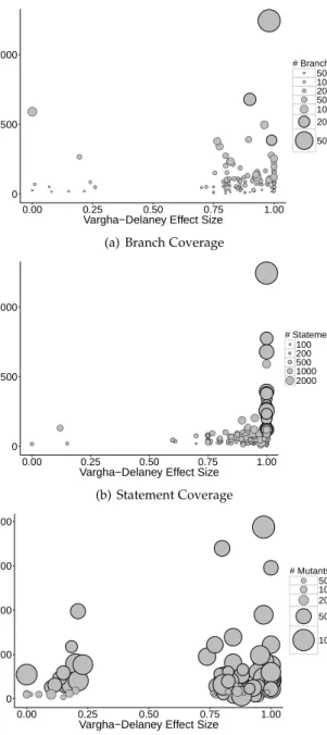
We carried out an empirical study on 346 Java classes using three coverage criteria (i.e., statement, branch, and strong mutation coverage) to assess the performance of DynaMOSA with respect to the whole-suite approach (WS), its archive-based variant (WSA) and MOSA. The results show that DynaMOSA outperforms WSA in 28% of the classes for branch coverage (+8% more coverage on average) and in 27% of the classes for mutation coverage (+11% more killed mutants on average). It outperforms WS in 51% of the classes for statement coverage, leading to +11% more coverage on average. Moreover, DynaMOSA outperforms its predecessor MOSA for all the three coverage criteria in 19% of the classes with +8% more code coverage on average.

Index Terms—Evolutionary Testing; Many-Objective Optimisation; Automatic Test Case Generation

F

1

I

Automated structural test case generation aims at producing a set of test cases that maximises coverage of the test goals in the software under test according to the selected adequacy testing criterion (e.g., branch coverage). Search-based test case generators use meta-heuristic optimisation algorithms, such as genetic algorithms (GA), to produce new test cases from the previously generated (initially, random) ones, so as to reduce and eventually nullify their distance from each of the yet uncovered targets [52], [37]. The search for a test sequence and for test input data that bring the test execution closer to the current coverage target is guided by a fitness function, which quantifies the distance between the execution trace of a test case and the coverage target. The actual computation of such a distance depends on the type of coverage criterion under consideration. For instance, for branch coverage, the distance is based on the number of control dependencies that separate the execution trace from the target (approach level) and on the variable values evaluated at the conditional expression where the execution diverges from the target (branch distance).

In traditional evolutionary testing, to cover all targets a meta-heuristic algorithm is applied multiple times, each

time with a different target, until all targets are covered or the total search budget is consumed. The final test suite is thus composed of all the test cases that cover one or more targets, including those that accidentally cover previously uncovered targets (collateral coverage).

Searching for one target at a time is problematic in several respects. First of all, targets may require higher or lower search effort depending on how difficult it is to produce test cases that cover them. Hence, uniformly distributing the search budget across all targets might be largely sub-optimal. Even worse, the presence of unfeasible targets wastes entirely the search time devoted to their coverage. Thewhole-suite(WS) approach [17], [3] to test case generation is a recent attempt to address these issues. WS optimises entire test suites, not just individual test cases, and makes use of a single fitness value that aggregates the fitness values measured for the test cases contained in a test suite, so as to take into consideration all coverage targets simultaneously. In fact, each test case in a test suite is associated with the target closest to its execution trace. The sum over all test cases of such minimum distances from the targets provides the overall, test-suite-level fitness. The additive combination of multiple targets into a single, scalar objective function is known as sum scalarization in

the theory of optimisation [11]. The aim is to apply single-objective algorithms, like GA, to an intrinsically multi-objective problem.

While being more effective than targeting one target at a time, the WS approach suffers all the well-known problems of sum scalarization in many-objective optimi-sation, among which the inefficient convergence occurring in the non-convex regions of the search space [11]. On the other hand, there are single-objective problem instances on which many-objective algorithms have been shown to be much more convenient than the single-objective approach. In fact, reformulating a complex single-objective problem as a many-objective problem defined on multiple but simpler objectives can reduce the probability that the search remains trapped in local optima, eventually leading to faster conver-gence [30], [21]. However, there are two main challenges to address when applying many-objective optimisation to test case generation: (i) none of the available multi or many-objective solvers can scale to the number of many-objectives (targets) typically found in coverage testing [3]; and (ii) multi and many-objective solvers are designed to increase the diversity of the solutions, not just to fully achieve each objective individually (reducing to zero its distance from the target), as required in test case generation [33].

To overcome the aforementioned limitations, in our pre-vious work [42] we introduced MOSA (Many-Objective Sorting Algorithm), a many-objective GA tailored to the test case generation problem. MOSA has three main features: (i) it uses a novelpreference criterioninstead of ranking the solutions based on their Pareto optimality; (ii) it focuses the search only on the yet uncovered coverage targets; (iii) it saves all test cases satisfying one or more previously uncovered targets into an archive, which contains the final test suite when the search ends.

Recently, Rojas et al. [48] developed the Whole Suite with Archive approach (WSA), a hybrid strategy that in-corporates some of MOSA’s routines inside the traditional WS approach. While WSA still applies the sum scalarization and works at the test suite level, it incorporates an archive strategy which operates at the test case level. Moreover, it also focuses the search only on the yet to cover targets. From an empirical point of view, WSA has been proved to be statistically superior to WS and to the one-target at a time approaches. However, from a theoretical point of view, it does not evolve test suites anymore since the final test suite given to developers is artificially synthesised by taking those test cases stored in the archive rather than returning the best individual (i.e., test suite) from the last generation of GAs [48]. Rojas et al. [48] arose the following still unanswered questions: (1)To what extent do the benefits of MOSA stem from the many-objective reformulation of the problem or from the use of the archiving mechanism?(2)How does MOSA performs compared to WSA since both of them implement an archiving strategy?

In this paper, we provide an in-depth analysis of many-objective approaches to test case generation, thus, answer-ing the aforementioned open questions. First, we present DynaMOSA (Many-Objective Sorting Algorithm with Dy-namic target selection) which extends MOSA with the capa-bility to dynamically focus the search on a subset of the yet uncovered targets, based on the control dependency

hierarchy. Thus, uncovered targets that are reachable from other uncovered targets positioned higher in the hierarchy are removed from the current vector of objectives. They are reinserted in the objective vector dynamically, when their parents are covered. Since DynaMOSA optimises a subset of the objectives considered by MOSA using the same many-objective algorithm and preference criterion, DynaMOSA is ensured to be equally or more efficient than MOSA.

Second, we conduct a large empirical study involving 346 Java classes sampled from four different datasets [18], [53], [49], [42] and considering three well known test ad-equacy criteria: statement coverage, branch coverage and mutation coverage. We find that DynaMOSA achieves sig-nificantly higher coverage than WSA in a large number of classes (27% and 28% for branch and mutation coverage respectively) with an average increment, for classes where statistically significant differences were observed, of +8% for branch coverage and +11% for mutation coverage. It also produces higher statement coverage than WS1in 51% of the classes, for which we observe +11% of covered statements on average. As predicted by the theory, DynaMOSA also improves MOSA for all the three criteria. This happens in 19% of the classes with an average coverage improvement of 8%.

This paper extends our previous work [42] with the following novel contributions:

1) DynaMOSA: a novel algorithm for dynamic target selection, which is theoretically proven as subsum-ing MOSA.

2) Larger scale experiments: one order of magnitude more classes are considered in the new experiments. 3) Empirical comparison of DynaMOSA with MOSA and WSA to provide support to the usage of many-objective solvers in addition to the archiving strat-egy, which is implemented in all the three ap-proaches.

4) Empirical assessment of the selected algorithms with respect to different testing criteria, i.e., branch coverage, statement coverage and strong mutation coverage.

5) Direct comparison with Pareto dominance ranking based algorithms, i.e., NSGA-II enriched with an archiving strategy.

6) Empirical assessment of our novel preference cri-terion, to understand if the higher effectiveness of DynaMOSA is due to the preference criterion alone or to its combination with dominance ranking. The remainder of this paper is organised as follows. Section 2 presents the reformulation of the test case gen-eration problem as a many-objective problem. Section 3 presents the many-objective test generator MOSA, followed by its extension, DynaMOSA, with dynamic selection of the coverage targets. Section 4 presents the description of the experiments we conducted for the evaluation of the proposed algorithm. Section 5 reports the results obtained from the experiments, while Sections 6 and 7 provide addi-tional empirical analyses and discuss the threats to validity,

1. For statement coverage, we consider WS as baseline since no implementation of WSA is available.

respectively. Section 8 summarises the research works most closely related to ours. Section 9 draws conclusions and identifies possible directions for future work.

2

P

F

This section presents our many-objective reformulation of the structural coverage problem. First the single-objective formulation used in the whole-suite approach [17] is de-scribed, followed by our many-objective reformulation, highlighting its main differences and peculiarities.

2.1 Single Objective Formulation

In the whole-suite approach, a candidate solution is a test suite consisting of a variable number of individual test cases, where each test case is a sequence of method calls of variable length. The fitness function measures how close the candidate test suite is to satisfy allcoverage targets(aka, test goals). It is computed with respect to full coverage (e.g., full branch coverage), as the sum of the individual distances to all coverage targets (e.g., branches) in the program under test. More formally, the problem of finding a test suite that satisfies all test targets has been defined as follows:

Problem 2.1: Let U = {u1, . . . , uk} be the set of structural test targets of the program under test. Find a test suite T =

{t1, . . . , tn}that minimises the fitness function: minfU(T) =X

u∈U

d(u, T) (1)

where d(u, T) denotes the minimal distance for the target u

according to a specific distance function.

In general, the function to minimise d is such that

d(u, T) = 0if and only if the target goal is covered when a test suiteT is executed. The difference between the various coverage criteria affects the specific distance function d

used to express how distant the execution traces are from covering the test targets in U when all test cases inT are executed.

In Branch Coverage, the test targets to cover are the conditional statement branches in the class under test. Therefore, Problem 2.1 can be instantiated as finding a test suite that covers all branches, using as function dthe traditional branch distance [37] for each individual branch to be covered. More formally [17]:

Problem 2.2: Let B = {b1, . . . , bk} be the set of branches in a class. Find a test suite T = {t1, . . . , tn} that covers all the feasible branches, i.e., one that minimises the following fitness function:

minfB(T) =|M| − |MT|+X

b∈B

d(b, T) (2)

where|M|is the total number of methods,|MT|is the number of executed methods by all test cases inT andd(b, T)denotes the minimal normalised branch distance for branchb∈B.

The term |M| − |MT| accounts for the entry edges of the methods that are not executed by T. The minimal

normalised branch distanced(b, t) for each branch b ∈ B

is defined as [17]: d(b, t) =         

0 if b has been covered

Dmin(t∈T, b)

Dmin(t∈T, b) + 1 if the predicate has been executed at least twice

1 otherwise

(3) whereDmin(t∈T, b)is the minimal non-normalised branch

distance, computed according to any of the available branch distance computation schemes [37]; minimality here refers to the possibility that the predicate controlling a branch is executed multiple times within a test case or by different test cases. The minimum is taken across all such executions. InStatement Coverage, the optimal test suite is the one that executes all statements in the code. To reach a given statement s, it is sufficient to execute a branch on which such a statement is directly control dependent. Thus, the distance functiondfor a statementscan be measured using the branch distances for the branches to be executed in order to reachs. More specifically, the problem is [17]:

Problem 2.3: LetS ={s1, . . . , sk}be the set of statements in a class. Find a test suite T = {t1, . . . , tn} that covers all the

feasible statements, i.e., one that minimises the following fitness function:

minfS(T) =|M| − |MT|+ X

b∈BS

d(b, T) (4)

where|M|is the total number of methods,|MT|is the number of

executed methods by all test cases inT;BS is the set of branches that hold a direct control dependency on the statements in S; andd(b, T)denotes the minimal normalised branch distance for branchb∈BS.

In Strong Mutation Coverage, the test targets to cover are mutants, i.e., variants of the original class obtained by injectingartificialmodifications (mimicking real faults) into them. Therefore, the optimal test suite is the one which is able to cover (kill, in the mutation analysis jargon) all mutants. A test case strongly kills a mutant if and only if the observable object state or the method return values differ between original and mutated class under test. Such a condition is usually checked by means of automatically generated assertions, which assert the equality of method return values and object state with respect to those observed when the original class is tested. Hence, such assertions fail when evaluated on the mutant if a different return value or object state is produced. An effective fitness functionf

for strong mutation coverage can be defined based on the notions of infection and propagation. The execution state of a mutated class instance is regarded asinfectedif it differs from the execution state of the original class when compared immediately after the mutated statement. This ensures that the mutant is producing some immediate effect on the class attributes or method variables, but it does not ensure that such an effect will propagate to an externally observable difference. Infectionpropagationaccounts for the possibility of observing a different state between mutant and original class in the statements that follow the mutated one along the execution trace. The corresponding formal definition is the following [19]:

Problem2.4: LetM ={m1, . . . , mk}be the set of mutants for

a class. Find a test suiteT ={t1, . . . , tn}that kills all mutants, i.e., one that minimises the following fitness function:

minfM(T) =fB_M(T) + X

m∈M

(di(m, T) +dp(m, T)) (5) wherefB_M(T)is the whole-suite fitness function for all branches inT holding a direct control dependency on a mutant in M;di

estimates the distance toward a state infection; anddpdenotes the

propagation distance.

From an optimisation point of view, in the whole-suite approach the fitness function f considers all the targets at the same time and aggregates all corresponding dis-tances into a unique fitness function by summing up the contributions from the individual target distances, i.e., the minimum distance from each individual target. In other words, multiple search targets are conflated into a single search target by means of an aggregated fitness function. Using this kind of approach, often namedscalarization[11], a problem which involves multiple targets is transformed into a traditional single-objective, scalar one, thus allowing for the application of single-objective meta-heuristics such as standard GA.

2.2 Many-Objective Formulation

In this paper, we reformulate the coverage criteria for test case generation as many-objective optimisation problems, where the objectives to be optimised are the individual distances from all the test targets in the class under test. More formally, in this paper we consider the following reformulation:

Problem2.5: LetU ={u1, . . . , uk}be the set of test targets to cover. Find a set of non-dominated test casesT ={t1, . . . , tn}

that minimise the fitness functions for all test targetsu1, . . . , uk,

i.e., minimising the followingkobjectives:

     minf1(t) =d(u1, t) .. . minfk(t) =d(uk, t) (6)

where each d(ui, t) denotes the distance of test case t from

covering the test target ui. Vector hf1, . . . , fki is also named

a fitness vector.

According to this new generic reformulation, branch coverage, statement coverage and strong mutation coverage can be reformulated as follows:

Problem 2.6: LetB ={b1, . . . , bk}be the set of branches of a class. Find a set of non-dominated test casesT = {t1, . . . , tn}

that minimises the fitness functions for all branchesb1, . . . , bk, i.e., minimising the followingkobjectives:

     minf1(t) =al(b1, t) +d(b1, t) .. . minfk(t) =al(bk, t) +d(bk, t) (7)

where each d(bj, t) denotes the normalised branch distance for the branch, executed by t, which is closest to bj (i.e., which is at minimum number of control dependencies frombj), while al(bj, t)is the corresponding approach level (i.e., the number of control dependencies between the closest executed branch andbj).

Problem 2.7: LetS ={s1, . . . , sk}be the set of statements in

a class. Find a set of non-dominated test casesT ={t1, . . . , tn}

that minimises the fitness functions for all statementss1, . . . , sk, i.e., minimising the followingkobjectives:

     minf1(t) =al(s1, t) +d(b(s1), t) .. . minfk(t) =al(sk, t) +d(b(sk), t) (8)

where each d(b(sj), t) denotes the normalised branch distance

of test case t for the branch closest to b(sj), the branch that

directly controls the execution of statement sj, while al(sj, t) is the corresponding approach level.

Problem2.8: LetM ={m1, . . . , mk}be the set of mutants for a class. Find a set of non-dominated test casesT ={t1, . . . , tn}

that minimises the fitness functions for all mutantsm1, . . . , mk, i.e., minimising the followingkobjectives:

             minf1(t) =al(m1, t) +d(b(m1), t) +di(m1, t)+ +dp(m1, t) .. . minfk(t) =al(mk, t) +d(b(mk), t) +di(mk, t)+ +dp(mk, t) (9)

where d(b(mj), t)and al(mj, t)denote the normalised branch distance and the approach level of test case t for mutant mj

respectively;di(mj, t)is the distance from state infection, while dp(mj, t)measures the propagation distance.

In this formulation, a candidate solution is a test case, not a test suite, which is scored by a single objective vector containing the distances from all yet uncovered test targets. Hence, the fitness is a vector ofkvalues, instead of a single aggregate score. In many-objective optimisation, candidate solutions are evaluated in terms of Pareto dominance and Pareto optimality[11]:

Definition 1: A test case xdominates another test casey (also writtenx≺y) if and only if the values of the objective function vector satisfy the following conditions:

∀i∈ {1, . . . , k} fi(x)≤fi(y) and

∃j∈ {1, . . . , k}such thatfj(x)< fj(y)

Conceptually, the definition above indicates that x is preferred to (dominates)yif and only ifxis strictly better on one or more objectives and it is not worse for the remaining objectives. For example, in branch coveragexis preferred to (dominates)yif and only ifxhas a lower branch distance + approach level for one or more branches and it is not worse for the remaining branches.

Figure 1 provides a graphical interpretation of Pareto dominance for a simple case with two test targets to cover, i.e., the problem is bi-objective. All test cases in the grey rectangle (AandC) are dominated byD, becauseDis better for both the two objectivesf1 and f2. On the other hand, the test caseD does not dominateB because it is closer to coverf1 than B, but it is worse than B on the other test target,f2. Moreover, D does not dominateE because it is worse for the test target f1. Similarly, the test caseB does

not dominateDandEbut it dominatesA. Thus,B,D, and

0 0.2 0.4 0.6 0.8 1 1.2 1.4 0 0.2 0.4 0.6 0.8 1 B A C D E f2=al(b2, t) +d(b2, t) f1 = al ( b1 , t ) + d ( b1 , t )

Fig. 1. Graphical interpretation of Pareto dominance.

Care dominated by eitherDorB. The test caseB satisfies (covers) the targetf2, thus, it is a candidate to be included in the final test suite.

Among all possible test cases, the optimal test cases are those non-dominated by any other possible test case:

Definition2: A test casex∗is Pareto optimal if and only if it is not dominated by any other test case in the space of all possible test cases (feasible region).

Single-objective optimisation problems have typically one solution (or multiple solutions with the same optimal fitness value). On the other hand, solving a multi-objective problem may lead to a set of Pareto-optimal test cases (with different fitness vectors), which, when evaluated, cor-respond to trade-offs in the objective space. While in many-objective optimisation it may be useful to consider all the trade-offs in the objective space, especially if the number of objectives is small, in the context of coverage testing we are interested in finding only the test cases that contribute to maximising the total coverage by covering previously uncovered test targets, i.e., test cases having one or more objective scores equal to zero:fi(t) = 0, as testBin Figure 1. These are the test cases that intersect any of themCartesian axes of the vector space where fitness vectors are defined. Such test cases are candidates for inclusion in the final test suite and represent a specific sub-set of the Pareto optimal solutions.

3

A

Search algorithms aimed at optimising more than three objectives have been widely investigated for classical nu-merical optimisation problems. A comprehensive survey of such algorithms can be found in a recent paper by Li et al.[34]. The following subsections provide a discussion of the most relevant related works on many-objective optimi-sation and highlight how our novel many-objective algo-rithm overcomes their limitations in the context of many-objective structural coverage. In particular, Section 3.1 pro-vides an overview on traditional many-objective algorithms, while Section 3.2 presents the many-objective algorithms

that we have developed for solving the many-objective reformulation of structural coverage criteria.

3.1 Existing Many-Objective Algorithms

Multi-objective algorithms, such as the Non-dominated Sorting Genetic Algorithm II (NSGA-II) [13] and the improved Strength Pareto Evolutionary Algorithm (SPEA2) [63], have been successfully applied within the software engineering community to solve problems with two or three objectives, including software refactoring, test case prioritisation, etc. However, such classical multi-objective evolutionary algorithms present scalability issues because they are not effective in solving optimisation problems with more than three-objectives [34].

To overcome their limitations, a number of many-objective algorithms have been recently proposed in the evolutionary computation community, which modify multi-objective solvers to increase the selection pressure. Ac-cording to Li et al. [34], existing many-objective solvers can be categorised into seven classes: relaxed dominance based, diversity-based, aggregation-based,indicator-based, refer-ence set based, preference-based, and dimensionality reduction approaches. For example, Laumanns et al. [33] proposed the usage of -dominance (-MOEA), which is a relaxed version of the classical dominance relation that enlarges the region of the search space dominated by each solution, so as to increase the likelihood for some solutions to be dominated by others [34]. Although this approach is helpful in obtaining a good approximation of an exponentially large Pareto front in polynomial time, it presents drawbacks and in some cases it can slow down the optimisation process significantly [27].

Yang et al. [58] introduced a Grid-based Evolutionary Algorithm (GrEA) that divides the search space into hyper-boxes of a given size and uses the concepts of grid domi-nance and grid distance to improve diversity among indi-viduals by determining their mutual relationship in a grid environment. Zitzler and K ¨unzli [62] proposed the usage of the hypervolume indicator instead of Pareto dominance when selecting the best solutions to form the next gener-ation. Even if the new algorithm, named IBEA (Indicator Based Evolutionary Algorithm), was able to outperform NSGA-II and SPEA2, the computation cost associated with the exact calculation of the hypervolume indicator in a high-dimensional space (i.e., with more than five objectives) is too expensive, making it unfeasible with hundreds of objectives as in the case of structural test coverage (e.g., in mutation coverage a class/program may have hundreds of mutants). Zhang and Li [61] proposed a Decomposition based Multi-objective Evolutionary Algorithm (MOEA/D), which decomposes a single many-objective problem into many single-objective sub-problems by employing a series of weighting vectors. Specifically, each sub-problem is ob-tained by using a specific weighting vector that aggregates different objectives using a weighted-sum approach. Differ-ent weighting vectors assign differDiffer-ent importance (weights) to objectives, thus, delimiting the searching direction of these aggregation-based algorithms. However, the selection of weighting vectors is still an open problem especially for problems with a very large number of objectives [34].

Di Pierro et al. [14] used a preference order-approach (POGA) as an optimality criterion in the ranking phase of NSGA-II. This criterion considers the concept of efficiency of order in subsets of objectives and provides a higher selection pressure towards the Pareto front than Pareto dominance-based algorithms.

Deb and Jain [12] proposed NSGA-III, an improved version of the classical NSGA-II algorithm, where the crowding distance is replaced with a reference-set based niche-preservation strategy. It results in a new Pareto rank-ing/sorting based algorithm that produces well-spread and diversified solutions.

Yuan et al. [59] developed θ-NSGA-III, which enriches the non-dominated sorting scheme with the concepts ofθ -dominance to rank solutions in the environmental selection phase, so as to ensure both convergence and diversity.

All the many-objective algorithms mentioned above have been investigated mostly for numerical optimisation problems with less than 15 objectives. Moreover, they are designed to produce a rich set of optimal trade-offs between different optimisation goals, by considering both proximity to the real Pareto optimal set and diversity between the obtained trade-offs [33]. As explained in Section 2.2, this is not the case of structural coverage for test case gener-ation. The interesting solutions for this problem are test cases having one or more objective scores equal to zero (i.e., fi(t) = 0). Trade-offs between objectives scores are

useful just for maintaining diversity during the optimisa-tion process. Hence, there are two main peculiarities that have to be considered in many-objective structural coverage as compared to more traditional many-objective problems. First, not all non-dominated test cases have a practical utility since they represent trade-offs between objectives. Instead, in structural coverage the search has to focus on a specific sub-set of the non-dominated solutions: those solutions (test cases) that satisfy one or more coverage targets. Second, for a given level of structural coverage, shorter test cases (i.e., test cases with a lower number of statements) are preferred to reduce the oracle cost [6], [17] and to avoid the bloat phenomenon [17].

3.2 The Proposed Many-Objective Algorithms

Previous research in many-objective optimisation [55], [34] has shown that many-objective problems are particu-larly challenging because of the dominance resistance phe-nomenon, i.e., most of the solutions are incomparable since the proportion of non-dominated solutions increases expo-nentially with the number of objectives. As a consequence, it is not possible to assign a preference among individuals for selection purposes and the search process becomes equiva-lent to a random one [55]. Thus, problem/domain specific knowledge is needed to impose an order of preference over test cases that are non-dominated according to the traditional non-dominance relation. For test case generation, this means focusing the search effort on those test cases that are closer to one or more uncovered targets (e.g., branches) of the program. To this aim, we propose the following preference criterionin order to impose an order of preference among non-dominated test cases:

Algorithm 1:NSGA-II

Input:

U={u1, . . . , um}the set of coverage targets of a program. Population sizeM

Result:A test suiteT

1 begin

2 t←−0// current generation

3 Pt←−RANDOM-POPULATION(M)

4 whilenot (search budget consumed)do

5 Qt←−GENERATE-OFFSPRING(Pt) 6 Rt←−PtSQt 7 F←−FAST-NONDOMINATED-SORT(Rt) 8 Pt+1←− ∅ 9 d←−1 10 while|Pt+1|+|Fd|6Mdo 11 CROWDING-DISTANCE-ASSIGNMENT(Fd) 12 Pt+1←−Pt+1SFd 13 d←−d+ 1

14 Sort(Fd) //according to the crowding distance 15 Pt+1←−Pt+1 S Fd[1 : (M− |Pt+1|)] 16 t←−t+ 1

17 S←−Pt

Definition3: Given a coverage targetui, a test casexis preferred over another test case y (also written x ≺ui y) if and only if

the values of the objective function for ui satisfy the following condition:

fi(x)< fi(y) OR fi(x) =fi(y)∧size(x)< size(y) where fi(x) denotes the objective score of test case x for

coverage targetui(see Section 2), andsizemeasures the test case length (number of statements). Thebest test casefor a given coverage targetuiis the one preferred over all the

oth-ers for such target (x_best ≺ui y, ∀y ∈T). Theset of best test

casesacross all uncovered targets ({x| ∃i:x≺u_i y, ∀y ∈ T}) defines a subset of the Pareto front that is given priority over the other non-dominated test cases in our algorithms. When there are multiple test cases with the same minimum fitness value for a given coverage targetui, we use the test case length (number of statements) as a secondary prefer-ence criterion. We opted for this secondary criterion since generated tests require human effort to check the candidate assertions (oracle problems). Therefore, minimising the test cases is a valuable (secondary) objective to achieve [6], [17] since smaller tests involve a lower number of method calls (and corresponding covered paths) to manually analyse.

Our preference criterion provides a way to distinguish between test cases in a set of non-dominated ones, i.e., in a set where test cases are incomparable according to the tradi-tional non-dominance relation, and it increases the selection pressure by giving higher priority to the best test cases with respect to the currently uncovered targets. Since none of the existing many-objective algorithms considers this prefer-ence ordering, which is a peculiarity of test case generation, in this paper we define our novel many-objective GA by incorporating the proposed preference criterion in the main loop of NSGA-II, a widely known Pareto efficient multi-objective genetic algorithm designed by Debet al.[13].

In a nutshell, NSGA-II starts with an initial set of random solutions (random test cases), also calledchromosomes, which represents a random sample of the search space (line 3 of Algorithm 1). The population then evolves through a series of generations to find better test cases. To produce the next generation, NSGA-II first creates new test cases,

calledoffsprings, by combining parts from two selected test cases (parents) in the current generation using thecrossover operator and randomly modifying test cases using the mu-tationoperator (function GENERATE-OFFSPRING, at line 5 of Algorithm 1). Parents are selected according to aselection operator, which uses Pareto optimality to give higher chance of reproduction to non-dominated (fittest) test cases in the current population. Thecrowding distance is used in order to make a decision about which test cases to select: non-dominated test cases that are far away from the rest of the population have higher probability of being selected (lines 10-15 of Algorithm 1). Furthermore, NSGA-II uses the FAST-NONDOMINATED-SORT algorithm to preserve the test cases forming the current Pareto frontier in the next generation (elitism). After some generations, NSGA-II converges to “stable” test cases, which represent the Pareto-optimal solutions to the problem.

The next sections describe in detail our proposed many-objective algorithms starting from NSGA-II, first describing the MOSA algorithm followed by its extension, DynaMOSA. 3.2.1 MOSA: a Many Objective Sorting Algorithm

MOSA (Many Objective Sorting Algorithm) replaces the tra-ditionalnon-dominated sortingwith a new ranking algorithm based on ourpreference criterion. As shown in Algorithm 2, MOSA shares the initial steps of NSGA-II: it starts with an initial set of randomly generated test cases that forms the initial population (line 3 of Algorithm 2); then, it cre-ates new test cases using crossover and mutation (function GENERATE-OFFSPRING, at line 6 of Algorithm 2).

Selection. Differently from NSGA-II, in MOSA the selec-tion is performed by considering both the non-dominance relation and the proposed preference criterion (function PREFERENCE-SORTING, at line 9 of Algorithm 2). In particular, the PREFERENCE-SORTING function, whose pseudo-code is provided in Algorithm 3, determines the test case with the lowest objective score (e.g., branch distance + approach level for branch coverage) for each uncovered tar-getui∈U, i.e., the test case that is closest to coverui(lines

2-6 of Algorithm 3). All these test cases are assigned rank 0 (i.e., they are inserted into the first non-dominated front F0), so as to give them a higher chance of surviving in to

the next generation (elitism). The remaining test cases (those not assigned to the first rank) are then ranked according to the traditional non-dominated sorting algorithm used by NSGA-II [13], starting with a rank equal to 1 and so on (line 11-15 of Algorithm 3). To speed-up the ranking procedure, the traditional non-dominated sorting algorithm is applied only when the number of test cases in F0 is smaller than

the population sizeM (condition in line 8). Instead, when the condition |_F0| > M is satisfied, the PREFERENCE-SORTING function returns only two fronts: the first front (rank 0) with all test cases selected by ourpreference criterion; and the front with rank 1 that contains all remaining test cases inT, i.e.,F1=T−F0.

Dominance. It is important to notice that the routine FAST-NONDOMINATED-SORT assigns the ranks to the remaining test cases by considering only the non-dominance relation for theuncoveredtargets, i.e., by focusing the search toward the interesting sub-region of the remaining search space. Such non-dominance relation is computed by a

Algorithm 2:MOSA

Input:

U={u1, . . . , um}the set of coverage targets of a program. Population sizeM

Result:A test suiteT

1 begin

2 t←−0// current generation

3 Pt←−RANDOM-POPULATION(M)

4 archive←−UPDATE-ARCHIVE(Pt,∅)

5 whilenot (search budget consumed)do

6 Qt←−GENERATE-OFFSPRING(Pt)

7 archive←−UPDATE-ARCHIVE(Qt, archive)

8 Rt←−PtSQt 9 F←−PREFERENCE-SORTING(Rt) 10 Pt+1←− ∅ 11 d←−0 12 while|Pt+1|+|Fd|6Mdo 13 CROWDING-DISTANCE-ASSIGNMENT(Fd) 14 Pt+1←−Pt+1SFd 15 d←−d+ 1

16 Sort(Fd) //according to the crowding distance 17 Pt+1←−Pt+1 S Fd[1 : (M− |Pt+1|)] 18 t←−t+ 1

19 T←−archive

Algorithm 3:PREFERENCE-SORTING

Input:

A set of candidate test casesT

Population sizeM

Result:Non-dominated ranking assignmentF

1 begin

2 F0// first non-dominated front 3 forui∈Uanduiis uncovereddo

4 // for each uncovered target we select the best test case

according to the preference criterion

5 tbest←−test case inTwith minimum objective score forui 6 F0←−F0S{tbest} 7 T←−T−F0 8 if|F0|> Mthen 9 F1←−T 10 else 11 U∗←− {g∈U: uis uncovered} 12 E←−FAST-NONDOMINATED-SORT(T ,{u∈U∗}) 13 d←−0//first front inE

14 forAll non-dominated fronts inEdo

15 Fd+1←−Ed

specific dominance comparator which iterates over all the uncovered targets when deciding whether two test cases

t1 and t2 do not dominate each other or whether one (e.g., t1) dominates the other (e.g., t2). While the original dominance comparator defined by Deb et al.[13] iterates all over the objectives (targets), in MOSA we use thedominance comparator depicted in Algorithm 4. Such a comparator iterates only over the uncoveredtargets (loop condition in line 4 of Algorithm 4). Moreover, as soon as it finds two uncovered targets for which two test casest1andt2do not dominate each other (lines 11-12 Algorithm 4), the iteration is terminated without analysing further uncovered targets.

Crowding distance. Once a rank is assigned to all can-didate test cases, thecrowding distanceis used to give higher probability of being selected to some test cases in the same front. As measure for the crowding distance, we use the sub-vector dominance assignmentproposed by K ¨oppen et al. [31] for many-objective optimisation problems. Specifically, the loop at line 12 in Algorithm 2 and the following lines 16 and 17 add as many test cases as possible to the next generation, according to their assigned ranks, until reaching

Algorithm 4:DOMINANCE-COMPARATOR

Input:

Two test cases to comparet1andt2

U={u1, . . . , um}the set of coverage targets of a program.

1 begin

2 dominates1←−false

3 dominates2←−false

4 forui∈Uanduiis uncovereddo

5 f1 i ←−values ofuifort1 6 f2 i ←−values ofuifort2 7 iff1 i < fi2then 8 dominates1←−true 9 iff2 i < fi1then 10 dominates2←−true

11 ifdominates1 == true & dominates2 == truethen

12 break

13 ifdominates1 == dominates2then

14 //t1andt2do not dominate each other 15 else

16 ifdominates1 == truethen

17 //t1dominatest2

18 else

19 //t2dominatest1

Algorithm 5:UPDATE-ARCHIVE

Input:

A set of candidate test casesT

An archiveA

Result:An updated archiveA

1 begin

2 forui∈Udo 3 tbest←− ∅ 4 best length←− ∞ 5 ifuialready coveredthen

6 tbest←−test case inAcoveringui

7 best length←−number of statements intbest 8 fortj∈Tdo

9 score←−objective score oftjfor targetui 10 length←−number of statements intj 11 ifscore== 0andlength≤best lengththen

12 replacetbestwithtjinA

13 tbest←−tj

14 best length←−length

15 returnA

the population size. The algorithm first selects the non-dominated test cases from the first front (F0); if the number

of selected test cases is lower than the population sizeM, the loop selects more test cases from the second front (F1),

and so on. The loop stops when adding test cases from current frontFd exceeds the population sizeM. At end of

the loop (lines 16-17), when the number of selected test cases is lower than the population sizeM, the algorithm selects the remaining test cases from the current frontFdaccording

to the descending order of crowding distance.

Archiving. As a further peculiarity with respect to other many-objective algorithms, MOSA uses a second popula-tion, calledarchive, to keep track of the best test cases that cover targets of the program under test. Specifically, when-ever new test cases are generated (either at the beginning of search or when creating offsprings) MOSA stores those tests that satisfy previously uncovered targets in thearchive as candidate test cases to form the final test suite (line 4 and 7 of Algorithm 2). To this aim, function UPDATE-ARCHIVE (reported in Algorithm 5 for completeness) updates the set

of test cases stored in thearchivewith the new generated test cases. This function considers both the covered targets and the length of test cases when updating thearchive: for each covered targetui it stores the shortest test case coveringui

in thearchive.

In summary, generation by generation MOSA focuses the search towards the uncovered targets of the pro-gram under test (both PREFERENCE-SORTING and FAST-NONDOMINATED-SORT routines analyse the objective scores of the candidate test cases considering the uncovered targets only); it also stores the shortest covering test cases in an external data structure (i.e., thearchive) to form the final test suite. Finally, since MOSA uses the crowding distance when selecting the test cases, it promotes diversity, which represents a key factor to avoid premature convergence toward sub-optimal regions of the search space [28]. 3.2.2 Graphical Interpretation

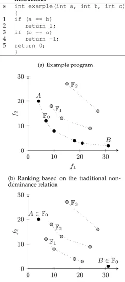
Let us consider the simple program shown in Figure 2-a. Let us assume that the coverage criterion is branch coverage and that the uncovered targets are the true branches of state-ments 1 and 3, whose branch predicates are(a == b)and

(b == c) respectively. According to the proposed many-objective formulation, the corresponding problem has two residual optimisation objectives, which are f1 = al(b1) +

d(b1) = abs(a−b)and f2 =al(b2) +d(b2) = abs(b−c).

Hence, any test case produced at a given generation g

corresponds to some point in a two-dimensional objective space as shown in Figure 2-b and 2-c. Unless bothaandbare equal, the objective functionf1computed using the combi-nation of approach level and branch distance is greater than zero. Similarly, functionf2is greater than zero unlessband care equal.

Let us consider the scenario reported in Figure 2-b where no test case is able to cover the two uncovered branches (i.e., in all cases f1 > 0 and f2 > 0). If we use the

traditional non-dominance relation between test cases, all test cases corresponding to the black points in Figure 2-b are non-dominated and form the first non-dominated front F0. Therefore, all such test cases have the same probability

of being selected to form the next generation, even if test case A is the closest to the Cartesian axis f2 (i.e., closest

to cover branch b2) and test case B is the closest to the

Cartesian axis f1 (branch b1). Since there is no preference among test cases in F0, it might happen that A and/or B are not kept for the next generation, while other, less useful test cases inF0 are preserved. This scenario is quite

common in many-objective optimisation, where the number of non-dominated solutions increases exponentially with the number of objectives [55]. However, from the branch coverage point of view the two test casesAandBare better (fitter) than all other test cases, because they are the closest to covering each of the two uncovered branches.

Our novel preference criteriongives a higher priority to test casesAandB with respect to all other test cases, guar-anteeing their survival in the next generation. In particular, using the new ranking algorithm proposed in this paper (see Algorithm 3), the first non-dominated frontF0will contain

only test cases A and B (see Figure 2-c), while all other test cases will be assigned to other, successive fronts. When there are multiple test cases that are closest to one axis,

Instructions

s int example(int a, int b, int c) { 1 if (a == b) 2 return 1; 3 if (b == c) 4 return -1; 5 return 0; }

(a) Example program

0 10 20 30 0 10 20 30 F0 A B F1 F2 f1 f2

(b) Ranking based on the traditional non-dominance relation 0 10 20 30 0 10 20 30 A∈F0 B∈F0 F1 F2 F3 f1 f2

(c) Ranking based on the proposed

prefer-ence criterion

Fig. 2. Graphical comparison between the non-dominated ranks assign-ment obtained by the traditionalnon-dominated sorting algorithmand the ranking algorithm based on thepreference criterionproposed in this paper.

associated with a given uncovered branch, the preference criterionprovides a further strategy to impose an order to the non-dominated test cases by assigning rank 0 to the shortest test case only.

3.2.3 DynaMOSA: Dynamic Selection of the Optimisation Targets

One main limitation in MOSA is that it considers all cover-age targets as independent objectives to optimise since the first generation. However, there exist structural dependen-cies among targets that should be considered when deciding which targets/objectives to optimise. For example, some targets can be satisfied if and only if other related targets are already covered.

To better explain this concept, let us consider the exam-ple in Figure 3. The four branches to be covered,b1, b2, b3, b4,

are not independent from each other. In fact, coverage of

b2, b3can be achieved only afterb1has been covered, since

Instructions

s int example(int a, int b, int c) { int x = 0; 1 if (a == b) //b1 2 if (a > c) //b2 3 x = 1; 4 else //b3 5 x = 2; 6 if (b == c) //b4 7 x = -1; 8 return x; }

(a) Example program

� � � � ���� � ���� � ���� � ����

(b) Control dependency graph

Fig. 3. Sinceb1holds a control dependency onb2, b3, targetsb2, b3are

dynamically selected only onceb1is covered.

the former targets are under the control of the latter. In other words, there is a control dependency betweenb1and

b2, b3, which means that the execution of b2, b3 depends

on the outcome of the condition at node 2, which in turn is evaluated only once target b1 is covered. If no test case coversb1, the ranking in MOSA is determined by the fitness

function f1 = d(b1). When tests are evaluated for the two dependent branches b2 and b3, the respective fitness functions will be equal tof1+ 1, since the only difference

from coverage ofb1consists of a higher approach level (in

this case, +1), while the branch distancedis the same. Since the values off2andf3are just shifted by a constant amount (the approach level) with respect tof1, the test case ranking

is the same as the one obtained when consideringf1alone. This means that taking into account objectivesf2, f3during preference sorting is useless, since they do not contribute to the final ranking.

The example illustrated above shows that coverage tar-gets can be organised into a priority hierarchy based on the following concepts in standard flow analysis:

Definition 4 (Dominator): A statement s1 dominates another

statements2if every execution path tos2passes throughs1.

Definition5(Post-dominator): A statements1post-dominates another statements2 if every execution path froms2 to the exit point (returnstatement) passes throughs1.

Definition6(Control dependency): There is a control depen-dency between program statements1 and program statements2

iff: (1)s2is not a postdominator ofs1and (2) there exists a path

in the control flow graph between s1 and s2 whose nodes are postdominated bys2.

Condition (1) in the definition of control dependency en-sures thats2is not necessarily executed afters1. Condition (2) ensures that once a specific path is taken between s1

ands2, the execution ofs2becomes inevitable. Hence,s1is

a decision point whose outcome determines the inevitable execution ofs2.

Definition 7 (Control dependency graph): The graphG =

hN, E, si, consisting of nodes n ∈ N that represent program statements and edges e ∈ E ⊆ N ×N that represent control dependencies between program statements, is called control de-pendency graph. Nodes∈N represents the entry node, which is connected to all nodes that are not under the control dependency of another node.

The definition of control dependency given above can be easily extended from program statements to arbitrary coverage targets. For instance, given two branches to be covered, b1, b2, we say b1 holds a control dependency on b2 ifb1 is postdominated by a statements1which holds a

control dependency on a nodes2that postdominatesb2. In DynaMOSA, the control dependency graph is used to derive which targets are independent from any others (targets that are free of control dependencies) and which ones can be covered only after satisfying previous targets in the graph. The difference between DynaMOSA and MOSA are illustrated in Algorithms 6. At the beginning the search process, DynaMOSA selects as initial set of objectives only those targets that are free of control dependencies (line 2). Once the initial population of random test cases is generated (line 4), the current set of targets U∗ is update using the routine UPDATE-TARGET highlighted in Algorithm 7. This routine is also called at each iteration in order to update the current set of targetsU∗to consider at each generation depending on the results of the execution of the offspring (line 10 in Algorithms 6). Therefore, fitness evaluation (line 8), preference sorting (line 12), and crowding distance (line 16) are computed only considering the targets inU∗⊆U.

The routine UPDATE-TARGET is responsible for dy-namically updating the set of selected targets U∗ so as to include any uncovered targets that are control dependent on the newly covered target. It iterates over all targets in

U∗ ⊆ U (loop in lines 2-6 of Algorithm 7) and in case of newly covered targets (condition in line 3) it visits the con-trol flow graph to find all concon-trol dependent targets. Indeed, Algorithm 7 uses a standard graph visit algorithm, which stops its visit whenever an uncovered target is encountered (lines 7-13). In such a case, the encountered target is added to the set of targetsU∗, to be considered by DynaMOSA in the next generation. If the encountered target is covered, the visit continues recursively until the first uncovered target is found or all targets have been already visited (lines 9-11). This ensures that only the first uncovered target, en-countered after visiting a covered target, is added to U∗. All following uncovered targets are just ignored, since the graph visit stops2_.

2. For simplicity, we only consider the case of targets associated with graph edges, but the same algorithm works if targets are associated with nodes

Algorithm 6:DynaMOSA

Input:

U={u1, . . . , um}the set of coverage targets of a program. Population sizeM

G=hN, E, si: control dependency graph of the program

φ:E→U: partial map between edges and targets

Result:A test suiteT

1 begin

2 U∗←−targets inUwith not control dependencies

3 t←−0// current generation

4 Pt←−RANDOM-POPULATION(M)

5 archive←−UPDATE-ARCHIVE(Pt,∅) 6 U∗←−UPDATE-TARGETS(U∗, G, φ)

7 whilenot (search budget consumed)do

8 Qt←−GENERATE-OFFSPRING(Pt)

9 archive←−UPDATE-ARCHIVE(Qt, archive)

10 U∗←−UPDATE-TARGETS(U∗, G, φ) 11 Rt←−PtSQt 12 F←−PREFERENCE-SORTING(Rt,U∗) 13 Pt+1←− ∅ 14 d←−0 15 while|Pt+1|+|Fd|6Mdo 16 CROWDING-DISTANCE-ASSIGNMENT(Fd,U∗) 17 Pt+1←−Pt+1SFd 18 d←−d+ 1

19 Sort(Fd) //according to the crowding distance 20 Pt+1←−Pt+1 S Fd[1 : (M− |Pt+1|)] 21 t←−t+ 1

22 T←−archive

Algorithm 7:UPDATE-TARGETS

Input:

G=hN, E, si: control dependency graph of the program

U∗⊆U: current set of targets

φ:E→U: partial map between edges and targets

Result:

U∗: updated set of targets to optimise

1 begin

2 foru∈U∗do 3 ifuis coveredthen 4 U∗←−U∗− {u}

5 eu←−edge inGfor the targetu

6 visit(eu)

7 Functionvisit(eu∈E)

8 foreach unvisiteden∈Econtrol dependent oneudo 9 ifφ(en)is not coveredthen

10 U∗←−U∗∪ {φ(en)}

11 setenas visited

12 else

13 visit(en)

In this way, the ranking performed by MOSA remains unchanged (a formal proof of this is provided below), while convergence to the final test suite is achieved faster, since the number of objectives to be optimised concurrently is kept smaller. Intuitively, the ranking of MOSA is unaffected by the exclusion of targets that are controlled by uncovered targets because such excluded targets induce a ranking of the test cases which is identical to the one induced by the controlling nodes.

There are two main conditions that must be satisfied to justify the dynamic selection of the targets produced by the execution of Algorithm 6:

1) Since at each generation, the set U∗ used by Dy-naMOSA contains all targets with minimum ap-proach level, for each remaining targetuiinU−U∗

there should exist a target u∗ ∈ U∗ such that

2) The computation cost of the routine UPDATE-TARGETS in Algorithm 7 should be negligible if compared to cost of computing preference sorting and crowding distance for the all uncovered targets. The first condition is ensured by Theorem 1, presented in the following. The second is not ensured theoretically, but it was found empirically to hold in practice.

DynaMOSA generates test cases with minimum distance from U∗, the set of uncovered targets directly reachable through a control dependency edge of one or more test case execution trace. On the other hand, MOSA generates test cases with minimum distance from the full set of uncovered targets, U. The two minimisation processes are equivalent if and only if the test cases at minimum distance from the elements ofU∗are also the test cases at minimum distance fromU. The following Theorem provides a theoretical justi-fication for the dynamic selection of a subset of the targets produced by the execution of Algorithm 7, by proving that the two sets of test cases optimised respectively by MOSA (Tmin) and DynaMOSA (T0) are the same.

Theorem1: LetUbe the set of all uncovered targets;Tminthe set

of test cases with minimum approach level fromUandT0the test cases with approach level zero;U∗be the set of uncovered targets at approach level zero from one or more test casest∈T0, then the

two sets of test casesTminandT0are the same, i.e.,Tmin=T0.

Proof: Since the approach level is always greater than or equal to zero, the approach level of the elements ofT0 is ensured to be

minimum. Hence,T0⊆Tmin. Let us now prove by contradiction that there cannot exist any uncovered target u associated with a test casetwhose approach level fromuis strictly greater than zero, such thattdoes not belong toT0. Let us consider the shortest path from the execution trace ofttouin the control dependency graph. The first nodeu0in such path belongs toU∗, since it is an uncovered target and it has approach level zero from the trace of

t. Indeed, it is an uncovered target because otherwise the test case

t0 that covers it would have an execution trace closer touthant. Since it satisfies the relation approach level(t, u0) = 0, test caset

must be an element ofT0. Hence,Tmincannot contain any test case not inT0and the equalityTmin=T0must hold.

Since the same set of test cases are at minimum distance from eitherU or U∗, the test case selection performed by MOSA, based on the distance of test cases fromU, is algo-rithmically equivalent to the test case selection performed by DynaMOSA, based on the distance of test cases fromU∗. The fact that DynaMOSA iterates over a lower number of targets (U∗ ⊆ U) with respect to MOSA has direct consequences on the computational cost of each single gen-eration. In fact, in each generation the two many-objective algorithms share two routines: the PREFERENCE-SORTING and the CROWDING-DISTANCE-ASSIGNMENT routines, as shown in Algorithms 2 and 6. For the fronts following the first one, the routine PREFERENCE-SORTING relies on the traditional FAST-NON-DOMINATED-SORT by Deb et al. [13] , which has an overall computation complexity of

O(M2_×N)

where M is the size of the population and

N is the number of objectives. Thus, for MOSA the cost of such routine is O(M2 _{× |U|) where U is the set of}

uncovered targets in a given generation. For DynaMOSA, the computational cost is reduced to O(M2× |U∗_{|) with} U∗ ⊆U being the set of uncovered targets with minimum

approach level. For trivial classes where all targets have no structural dependencies (i.e., classes with only branchless methods), the cost of PREFERENCE-SORTING will be the same since U∗ = U. However, for non-trivial classes we would expectU∗ ⊂U leading to a reduced computational complexity.

A similar analysis can be performed for the other shared routine, i.e., CROWDING-DISTANCE-ASSIGNMENT. Ac-cording to K ¨oppen et al. [31], the cost of such a routine when using the sub-vector dominance assignment is O(M2 _×N)

whereM is the size of the population whileNis the number of objectives. Therefore, for MOSA the cost of such routine isO(M2_{× |U|)}

whereUis the set of uncovered targets in a given generation; while for DynaMOSA it isO(M2× |U∗_|).

For non-trivial classes, DynaMOSA will iterate over a lower number of targets as long as the conditionU∗⊂U holds.

Moreover, MOSA requires to compute the fitness scores (e.g., approach level and branch distances in branch cover-age) for all uncovered targetsU and for each newly gener-ated test case. In particular, for each test case MOSA requires to compute the distances between execution traces and all targets inU. Instead, DynaMOSA focuses only on coverage targets with minimum approach levels, thus, requiring to compute the fitness scores forU∗⊆Uonly.

The additional operations of DynaMOSA with respect to MOSA are the construction of the intra-procedural control dependency graph and its visit for target selection. The cost for intra-procedural control dependency graph construction is paid just once for all test case generation iterations and the computation of the graph can be carried out offline, before running the algorithm. The visit of the control de-pendency graph for coverage target selection can be per-formed very efficiently (for structured programs the graph is a tree). As a consequence, the saving in the computa-tion of PREFERENCE-SORTING, CROWDING-DISTANCE-ASSIGNMENT and fitness scores performed by DynaMOSA vs. MOSA is expected to dominate the overall execution time of the two algorithms, while the visit of the control dependency graph performed by DynaMOSA is expected to introduce a negligible overhead. This was confirmed by our experiments. In fact, in our experiments the intra-procedural control dependency graphs of the methods under test and their visit consumed a negligible amount of execution time in comparison with the time taken by the extra computa-tions performed by MOSA.

4

E

E

This section details the empirical study we carried out to evaluate the proposed many-objective test case generation algorithms with respect to three testing criteria: (i) branch coverage, (ii) statement coverage, and (iii) strong-mutation coverage.

4.1 Subjects

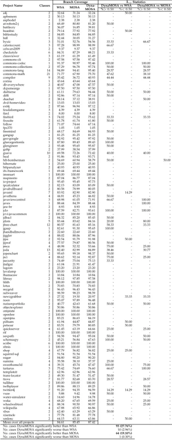
Thecontextof our study is a random selection of classes from four test benchmarks: (i) the SF110 corpus [18]; (ii) the SBST tool contest 2015 [53]; (iii) the SBST tool contest 2016 [49]; and (iv) the benchmark used in our previous conference paper [42].

The SF110 benchmark3 _{is a corpus of Java classes} com-posed of a representative sample of 100 projects from the SourceForge.net repository, augmented with 10 of the most popular projects in the repository, for a total of 23,886 classes. We selected this benchmark since it has been widely used in the literature to assess test case generation tools [18], [51], [48]. However, Shamshiri et al. [51] showed that the vast majority of classes in the FS110 corpus are trivial to cover fully, even with random search algorithms. In fact, they observed that most of the classes in this corpus do not require the usage of evolutionary algorithms. Hence, for our evaluation we selected only non-trivial classes from this benchmark. To this aim, we first computed the McCabe’s cyclomatic complexity [36] for each method in FS110 by means of the extendedCKJMlibrary4. The McCabe’s cyclo-matic complexity of a method is defined as the number of independent paths in the control flow graph and can be shown (for structured programs) to be equal to the number of branches plus one. We found that 56% of the classes in SF110 are trivial, containing only methods with cyclomatic complexity equal to 1. These are branchless methods that can be fully covered by a simple method call. Therefore, we pruned this benchmark by removing all classes whose methods have a cyclomatic complexity lower than five5. This filtering resulted in a smaller benchmark composed of 96 projects and 23% of classes from the original SF110 corpus. Among those 96 projects, 18 projects contain only a single non-trivial class after our filter. For our experiment, we randomly sampled 2 classes from each of the 78 projects containing multiple non-trivial classes, and we selected the available non-trivial classes from each of the remaining 18 projects. In addition, we randomly sampled two further classes for each of the most popular projects (11 projects), and one additional class for each of the eight larger projects in the repository. This resulted in 204 non-trivial classes.

From the latest two editions of the SBST unit test tool contests [53], [49] we selected 97 subjects: 46 classes from the third edition [53] and 51 classes from the fourth edition [49] of the contest. From the original set of classes in the two competitions, we removed all duplicate classes belonging to different versions of the same library since we would not expect any relevant difference over different versions in terms of branch, statement, or mutation coverage. We selected these two benchmarks because they contain java classes with different characteristics and belonging to dif-ferent application domains. In addition, they have been recently used to assess the performance of different test generation techniques.

Our last benchmark is the one used in our previous conference paper [42], from which we consider all classes used in our previous empirical study. While the original dataset includes 64 classes, in the present study we report the results for 45 classes, since 19 classes are shared with the SF110 corpus and with the latest SBST unit test tool contest [49].

In total, the selected 346 Java classes have 360,941 state-ments, 61,553 branches, and 117,816 mutants that are

consid-3. http://www.evosuite.org/experimental-data/sf110/ 4. http://gromit.iiar.pwr.wroc.pl/p inf/ckjm/

5. A method with cyclomatic complexity equal to five contains at least twoconditionalstatements.

TABLE 1

Java projects and classes in our study

Project Name Classes Branches Statements Mutants

Min Mean Max Min Mean Max Min Mean Max

a4j 2 31 78 125 231 1134 2038 15 477 940 apbsmem 2 41 215 390 283 2303 4323 315 371 427 asphodel 1 42 42 42 353 353 353 84 84 84 at-robots2-j 2 37 81 125 512 672 832 233 336 439 battlecry 2 78 179 281 1588 1947 2306 349 604 859 beanbin 2 41 44 47 242 298 355 114 128 142 biblestudy 2 33 35 37 280 381 483 151 193 236 biff 1 817 817 817 7012 7012 7012 488 488 488 bpmail 1 27 27 27 215 215 215 51 51 51 byuic 4 39 357 740 296 2038 4846 59 281 664 caloriecount 3 25 94 232 58 541.67 1425 5 311 909 celwars2009 2 11 185 360 135 1137 2139 39 448 857 checkstyle 6 9 41 111 92 294 412 16 214 517 classviewer 3 60 155 235 327 1219 2315 208 451 630 commons-cli 2 133 146 159 605 788 972 323 407 492 commons-codec 1 504 504 504 2385 2385 2385 725 725 725 commons-collections 3 28 113 221 276 389 576 289 671 904 commons-lang 14 40 309 1163 216 1543 5348 125 571 1086 commons-math 21 26 104 266 165 952 3184 57 467 979 compiler 9 73 293 758 121 1178 3734 151 448 787 corina 1 55 55 55 282 282 282 152 152 152 db-everywhere 2 13 83 153 97 900 1704 13 297 582 dcparseargs 1 80 80 80 571 571 571 220 220 220 diebierse 2 27 54 81 250 636 1022 39 213 388 diffi 2 20 27 35 152 248 344 214 241 268 dsachat 2 69 83 98 857 880 904 319 375 432 dvd-homevideo 3 29 55 84 947 1188 1386 52 82 98 ext4j 2 11 75 139 69 463 857 58 161 265 feudalismgame 3 11 285 788 104 1796 4873 99 159 226 fim1 2 25 49 73 170 655 1140 37 100 163 firebird 3 99 445 1040 581 2698 6591 0 245 387 fixsuite 2 35 54 74 335 483 631 108 204 301 follow 2 20 27 35 108 214 321 449 489 529 fps370 2 70 110 151 668 1320 1973 726 807 888 freemind 2 29 118 208 434 1027 1621 132 476 820 gangup 1 32 32 32 438 438 438 191 191 191 geo-google 2 24 27 30 44 95 147 20 59 99 gfarcegestionfa 2 76 99 123 503 826 1150 146 515 884 glengineer 2 23 69 115 325 491 658 154 267 380 gsftp 2 29 60 91 191 650 1110 104 471 839 guava 11 28 115 325 46 385 1114 53 390 886 heal 2 38 106 175 448 1155 1863 88 174 261 hft-bomberman 2 13 70 128 134 491 849 21 86 151 hibernate 1 4 4 4 62 62 62 6 6 6 httpanalyzer 2 56 128 200 656 2824 4992 407 537 667 ifx-framework 1 72 72 72 462 462 462 139 139 139 imsmart 1 15 15 15 69 69 69 29 29 29 inspirento 2 27 61 95 327 488 649 221 331 441 io-project 1 66 66 66 282 282 282 96 96 96 ipcalculator 2 55 79 103 1077 1252 1428 300 362 425 javabullboard 2 98 119 141 715 942 1170 432 445 458 javaml 7 12 39 56 120 303 448 58 194 273 javathena 4 49 206 330 197 1995 4279 65 372 784 javaviewcontrol 3 32 876 2373 179 2989 7027 91 446 712 javex 1 173 173 173 1023 1023 1023 208 208 208 jaw-br 2 28 38 48 196 232 269 61 78 95 jclo 1 133 133 133 987 987 987 383 383 383 jcvi-javacommon 2 29 45 61 232 236 240 169 251 334 jdbacl 2 188 193 198 1339 1475 1611 592 653 715 jdom 5 50 111 264 168 592 1116 18 298 895 jfree-chart 12 13 235 1005 74 1647 6610 18 488 907 jgaap 1 23 23 23 1245 1245 1245 59 59 59 jhandballmoves 2 26 29 32 234 307 380 23 41 60 jiggler 4 33 70 118 459 648 1205 211 555 985 jipa 2 24 79 134 124 453 783 87 241 395 jiprof 4 76 451 824 430 2612 5299 160 499 774 jmca 4 199 2515 7939 966 5887 16624 0 329 559 joda 13 53 214 697 366 1003 1892 152 469 866 jopenchart 2 20 56 92 241 690 1139 72 300 529 jsci 4 84 245 436 760 2331 3756 223 597 980 jsecurity 3 36 91 170 207 444 725 167 272 438 jtailgui 2 13 18 23 158 244 331 21 107 193 jwbf 2 45 48 52 225 312 399 101 109 117 lagoon 2 63 64 65 675 841 1007 80 97 115 lavalamp 1 18 18 18 122 122 122 61 61 61 lhamacaw 2 23 46 70 416 565 714 115 144 174 liferay 2 78 85 93 406 434 462 55 160 266 lilith 1 134 134 134 496 496 496 183 183 183 lotus 2 24 26 28 122 123 125 12 31 51 mygrid 2 28 28 28 113 113 113 35 35 35 netweaver 2 69 71 73 249 284 320 46 100 155 newzgrabber 3 32 126 268 404 973 1552 48 301 625 noen 2 67 69 71 316 456 597 145 200 256 nutzenportfolio 2 21 34 48 817 856 895 78 104 131 objectexplorer 2 17 96 175 47 517 987 48 147 246 omjstate 1 30 30 30 139 139 139 34 34 34 openhre 2 50 73 97 220 577 934 143 198 253 openjms 2 34 67 101 190 540 891 70 129 189 pdfsam 2 19 30 41 248 313 378 57 83 110 petsoar 2 16 31 47 61 182 303 56 79 102 quickserver 4 69 218 501 488 1669 3697 15 257 747 resources4j 1 176 176 176 1539 1539 1539 714 714 714 rif 1 21 21 21 94 94 94 56 56 56 saxpath 2 55 269 484 115 574 1034 128 393 659 schemaspy 2 17 198 380 140 1190 2241 21 311 602 scribe 6 2 13 37 14 113 355 1 24 47 sfmis 1 32 32 32 437 437 437 427 427 427 shop 4 41 108 192 316 828 1329 175 303 465 squirrel-sql 2 21 36 51 51 90 130 93 100 108 sugar 2 24 37 51 113 298 484 8 75 142 summa 4 30 197 372 185 1222 2114 95 357 680 sweethome3d 4 155 339 619 841 1913 3368 165 433 675 tartarus 3 228 344 514 1164 2094 3775 638 835 942 templateit 2 31 42 54 123 258 394 59 86 113 trans-locator 2 23 28 34 297 424 551 214 339 464 trove 10 0 124 281 232 683 1842 109 683 999 tullibee 2 20 20 21 97 101 106 175 186 198 twfbplayer 2 74 115 156 424 839 1255 383 402 422 twitter4j 7 25 104 319 227 1313 6320 107 257 401 vuze 2 119 126 134 657 666 675 292 387 482 water-simulator 2 59 98 137 888 1162 1436 274 606 939 weka 4 29 338 809 274 2773 7809 126 405 793 wheelwebtool 4 40 272 817 371 1598 3944 77 392 679 wikipedia 4 19 35 72 61 325 796 52 143 394 xbus 2 18 23 28 170 219 269 54 68 83 xisemele 1 27 27 27 152 152 152 70 70 70 xmlenc 2 182 698 1214 693 1439 2186 466 657 848 Total 346

ered as coverage targets in our experiment. Table 1 reports the characteristics of the selected classes, grouped by project. Specifically, it reports the number of classes selected for each project as well as minimum, average (mean), and maximum number of statements, branches and mutants contained in