in Low Resource Languages
Master’s thesis in Computer science and engineeringDAVID RODRIGUEZ
DENITSA SAYNOVA
Department of Computer Science and Engineering CHALMERSUNIVERSITY OF TECHNOLOGY
Machine Learning for Detecting Hate Speech in
Low Resource Languages
DAVID RODRIGUEZ
DENITSA SAYNOVA
Department of Computer Science and Engineering
Chalmers University of Technology University of Gothenburg
DENITSA SAYNOVA
© DAVID RODRIGUEZ DENITSA SAYNOVA, 2020.
Supervisor: Richard Johansson, Department of Computer Science and Engineering Examiner: K V S Prasad, Department of Computer Science and Engineering
Master’s Thesis 2020
Department of Computer Science and Engineering
Chalmers University of Technology and University of Gothenburg SE-412 96 Gothenburg
Telephone +46 31 772 1000
Typeset in LATEX
DENITSA SAYNOVA
Department of Computer Science and Engineering
Chalmers University of Technology and University of Gothenburg
Abstract
This work examines the role of both cross-lingual zero-shot learning and data aug-mentation in detecting hate speech online for low resource set-ups. The proposed solutions for situations where the amount of labeled data is scarce are to use a language with more resources during training or to create synthetic data points. Cross-lingual zero-shot results suggest some knowledge transfer is occurring. How-ever, results seem greatly influenced by the specific training data set selected. This is further supported by cross-data set experimentation within the same language, where results were also found to fluctuate based on training data without the need for cross-lingual transfer. Meanwhile, data augmentation methods show an im-provement, especially for low amounts of data. Furthermore, a detailed discussion on how the proposed data augmentation techniques impact the data is presented in this work.
Keywords: machine learning, natural language processing, BERT, cross-lingual zero-shot learning, data augmentation, hate speech, classification, Twitter
The authors would like to thank Richard Johansson for his support and feedback throughout this project and KVS Prasad for the many constructive discussions.
List of Figures xi
List of Tables xiii
1 Introduction 1 2 Theory 3 2.1 Machine Learning . . . 3 2.1.1 Unsupervised Learning . . . 4 2.1.2 Supervised Learning . . . 4 2.1.2.1 Data Annotation . . . 5 2.2 Feature Representations . . . 6
2.3 Neural Networks for Text Representations . . . 7
2.3.1 Neural Network Basics . . . 7
2.3.2 Transformers . . . 8 2.4 Transfer Learning . . . 10 2.4.1 BERT . . . 11 2.5 Cross-Lingual Representations . . . 12 2.5.1 Multilingual BERT . . . 12 2.6 Data Augmentation . . . 13
2.6.1 TF-IDF Synonym Replacement . . . 14
2.6.2 Word Dropout . . . 15
2.6.3 Back-Translation . . . 16
3 Methods 17 3.1 Hate Speech Data Sets . . . 17
3.1.1 Annotation Guidelines . . . 17
3.2 Baseline . . . 19
3.3 Cross-Lingual Zero-Shot Learning . . . 20
3.4 Effects of Training Set Size on Performance . . . 20
3.5 Data Augmentation . . . 20
3.5.1 TF-IDF Synonym Replacement . . . 21
3.5.2 Word Dropout . . . 21
3.5.3 Back-Translation . . . 21
3.6 Translation of English Training Data . . . 22
3.7 Evaluation . . . 22
3.8.1 Clustering . . . 23
3.8.1.1 Clustering for Hate Speech . . . 24
3.8.1.2 Clustering English Training Data Sets . . . 25
3.8.2 Classifying English Training Data Sets . . . 25
4 Results 27 4.1 Baseline . . . 27
4.2 Cross-Lingual Zero-Shot Learning . . . 28
4.3 Effects of Training Set Size on Performance . . . 30
4.4 Data Augmentation . . . 30
4.4.1 TF-IDF Synonym Replacement . . . 31
4.4.2 Word Dropout . . . 31
4.4.3 Back-Translation . . . 32
4.5 Translation of English Training Data . . . 32
4.6 Data Set Analyses . . . 33
4.6.1 Clustering . . . 33
4.6.1.1 Clustering of HatEval Data Sets . . . 33
4.6.1.2 Clustering English Training Data Sets . . . 35
4.6.2 Classifying English Data Sets . . . 37
5 Discussion 39 5.1 Cross-Lingual Zero-Shot Learning . . . 39
5.2 Data Augmentation . . . 40
5.2.1 TF-IDF Synonym Replacement . . . 40
5.2.2 Word Dropout . . . 41
5.2.3 Back-Translation . . . 42
5.3 Translation of English Training Data . . . 43
5.4 Data Set Analyses . . . 44
5.4.1 Clustering of HatEval Data Sets . . . 44
5.4.2 Clustering English Training Data Sets . . . 44
5.5 Classifying English Data Sets . . . 45
6 Conclusion 47
Glossary 49
2.1 Examples of less useful (left) and more useful (right) feature
repre-sentations. . . 6
2.2 An example of a neural network. . . 7
2.3 An example of a recurrent neural network [29]. . . 8
2.4 An example of the transformer architecture where both on the left and on the right side, several of the components are stacked on top of each other. . . 9
2.5 An example of transfer learning. The main model is used to identify the breed of dogs. The knowledge gained could be useful for identi-fying breeds of cats, however, it is probably not useful for identiidenti-fying healthy brains in MRI images. . . 11
2.6 BERT input representation, where the input is a sum of three levels of embedding [8]. . . 12
2.7 The original image. . . 13
2.8 Original image blurred. . . 13
2.9 Original image blurred too much. . . 13
3.1 Example of true positive and negative elements versus selected pos-itives and negatives. The green and red points refer to positive and negative true labels, respectively. While the green and red back-grounds refer to what the model considers positive and negative, re-spectively. . . 22
3.2 Purity and inverse purity calculation for the three clusters above. Majority class for each cluster: cluster A:N, 5; cluster B:, 4; cluster C: F, 3. Purity = 201(5+4+3) ≈ 0.6. Majority label for each class: N: cluster A, 5 : cluster B, 4 F: cluster A, 4. Inverse purity = 1 20(5+4+4) ≈ 0.65. . . 24
3.3 Distribution of data compared to labels when perfect correlation is observed. . . 25
4.1 Spanish base grid search. Darkest green indicates highest accuracy value – 83.73. . . 27
4.2 English base grid search. Darkest green indicates highest accuracy value – 80.75. . . 27
4.3 Size dependence of performance for Spanish data. . . 30
4.4 Distribution of tweets within all available English data sets in each cluster. . . 36
4.5 Distribution of hate and non-hate tweets within all available English data set in each cluster. . . 36
2.1 Example of data that requires annotation. The tweet’s text is the only thing that is automatically acquired. The label is obtained through
manual annotation (neg = negative; pos = positive). . . 5
2.2 Example of multiple annotations. The label requires the decisions from each individual annotator – A1, A2 and A3 (neg = negative; pos = positive) and is based on the majority vote. . . 5
2.3 Values of TF-IDF scores for example given above. . . 14
3.1 A confusion matrix with two classes . . . 26
4.1 Performance of the English Base (EN) and Spanish Base (ES). . . 28
4.2 Performance of English and Spanish base on other languages. Base-lines with no cross-lingual learning are shown in gray. . . 28
4.3 Performance of different English models. Baselines on own test sets are shown in gray. WH refers to [26], F refers to [11] and HatEval refers to [3]. . . 29
4.4 Performance of Waseen & Hovy data set on other languages. Baseline with no cross-lingual learning are shown in gray. . . 29
4.5 Performance of Founta data set on other languages. Baseline with no cross-lingual learning are shown in gray. . . 30
4.6 Validation set TF-IDF results. Baselines where no DA is applied are shown in gray. . . 31
4.7 Results obtained using word dropout. Baselines where no DA is ap-plied are shown in gray. . . 32
4.8 Results obtained using back-translation. Baselines where no DA is applied are shown in gray. . . 32
4.9 Translated vs cross-lingual zero-shot results. . . 33
4.10 Clustering results for hate speech in English training HatEval data. . 34
4.11 Clustering results for hate speech in Spanish training HatEval data. . 34
4.12 Clustering results for data source in English training data. . . 35
4.13 Clustering results for hate speech in English training data. . . 35
4.14 Data source classification results. Showing number of data points having a particular label vs the model prediction. Standard deviation on those counts are also shown in parentheses. . . 37 A.1 Performance of English Base (EN) and Spanish Base (ESP). . . I A.2 Performance of English and Spanish base on other languages. . . I
A.3 Results obtained using different English Sets. . . I A.4 Cross-lingual zero-shot results obtained using Founta. . . II A.5 Cross-lingual zero-shot results obtained using Waseem & Hovy. . . II A.6 Results obtained using word dropout. . . II A.7 Results obtained using back-translation. . . II A.8 Translated vs cross-lingual zero-shot results. . . II A.9 Performance of English trained model for sentiment analysis. . . III
1
Introduction
Hate speech online is increasingly becoming a bigger problem in recent years [16] and has long been a conductor towards different types of hate crimes.1 Even though
there is no exact definition that is universally accepted, hate speech tends to be broadly defined as a type of communication where a person or a group of people gets denigrated based on race, gender or sexual orientation amongst other factors.
In recent years, most social media companies have been heavily criticized for their handling of hate speech within their platform.2 As hate speech is expressed
through language, applying natural language processing (NLP) techniques can be very beneficial for managing it. NLP is a set of computational tools for language understanding, which can be helpful for automating the detection of hate speech. Given the complexity of patterns in hate speech, it is not feasible to develop a purely procedural approach for detecting it. An important component of a solution for similar problems is to also apply machine learning (ML). ML is an approach to building models that change through experience, i.e. automatically learn patterns from example training data. Therefore the performance of ML models is tightly related to the amount and quality of the example data provided. In this case a classification model is used, which outputs a label given a piece of text as input.
Since the task at hand is concerned with classifying data, the examples needed for training the model have to be annotated. This is typically done by multiple people giving each data point a label and choosing the majority. Most of these available examples that are labeled tend to be in English. However, social media is multilingual and the question of moderating all media content is an important one. Therefore, the current work focuses on solutions for hate speech discovery online in languages where resources available are scarce.
Two solutions that are explored are data augmentation (DA) and cross-lingual zero-shot learning. The former is a method for producing additional data examples by transforming existing ones. Thus, increasing the amount of available examples without the need for additional collection or labeling. The latter trains a model using a language different than the one the model is applied to. For instance, the model is trained on English hate speech examples in order to detect Spanish hate speech. This leads to the possibility of using a more populous data set for training. The development of these techniques comes with a unique set of challenges.
1https://www.nytimes.com/2018/10/15/technology/myanmar-facebook-genocide.html 2https://www.businessinsider.com/jack-dorsey-twitter-abuse-ted-2019-4?r=US&IR=T
One of the main issues is related to the specific details of the hate speech definition. This is because each data set uses slightly different guidelines when labeling the data. Secondly, as the labels are determined by a group of people and hate speech is complex, there tends to be low annotation agreement – i.e. the annotators tend to disagree on the correct label. Additionally, there might be cultural differences when perceiving hate speech which could impair the transferability of annotations from one culture to another.
Furthermore, some of the issues stem purely from the nature of the data. For example, social media text presents unique challenges since it has a distinct language structure like abbreviations, slang, typos, punctuation issues, etc. [9]
Since this is a complex task, there are several aspects that are not explored in full detail. One of these is the role of the similarity between the training and testing language in the cross-lingual zero-shot experiments. It can be assumed that lan-guages from within the same family work better than two from different ones. How-ever, testing the role of language proximity on performance is very time-consuming. Another issue with the current set-up is the quality of the annotations. Since these are manual, the quality could vary substantially between data sets. The effects of this issue are discussed in the current work. However, developing possible solutions is outside the scope of this project.
In order to best present the project, its components are discussed in the fol-lowing order: Chapter 2 introduces the main theoretical concepts used; Chapter 3 outlines the experimental set-up; Chapter 4 presents the obtained results; Chapter 5 consists of a discussion of said results; Chapter 6 summarizes the project and lays out possible direction for further works.
2
Theory
In this chapter, some background of the theoretical framework needed is outlined. This includes the key ideas concerning both data annotation and machine learning. A deeper background is given in particular for transfer learning and the model used in this project. Finally, a description of the two methods used for dealing with scarce data – cross-lingual zero-shot learning and data augmentation – is presented.
2.1
Machine Learning
Machine learning is a field that utilizes data to build models for automatic decision making. A model can be seen as a black box that is fed values of an inputx (called features) and produces an output decision y. In reality, that black box can have a variety of different architectures that are suited for different tasks and can be seen as complex functions mapping the input to the output. Initially, before data is introduced, the model can be seen as simply knowing the type of the function without knowing the values of the parameters.
There are two main types of machine learning, supervised and unsupervised learning (discussed in more detail in sections 2.1.1 and 2.1.2, respectively). The main distinction is the availability of a label (quantity of interest) for each data point example, i.e. having examples of correct (x, y) pairs. Supervised learning is carried out in cases when a label is available for the training examples, whereas unsupervised learning is applied to cases with no available label.
An example of a supervised task is classifying inputs into two groups, where the model used could be the perceptron. This uses a function of the form:
y(x) = 1 w.x+b > 0 0 otherwise
As can be seen, the model determines the general relationship between the input
x and the output y, without giving the specific values of the parameters w and b. These are found through a process called training, which consists of the following steps:
• passing the input through the model and obtaining a prediction • comparing the prediction to the input’s true label
• based on the difference between the prediction and the true label, modify the parameters
The specific modification the parameters go through is determined by the model’s architecture. In the case of the perceptron if the prediction and the true label match, the weights are not changed. However when the prediction and the true label do not match, for a positive true label the weights are made more positive and for a negative true label the weights are made more negative. This is done to encourage the prediction towards the correct label.
In order to obtain more stable values for the parameters, this process needs to be repeated for all available data points several times. The amount of times the data is passed through the model is a hyper-parameter that is pre-set, i.e. not learned from the data. However, setting that number to a very high value on a small data set can lead to learning just the specific examples given. For this reason, a big enough data set with variability is needed in order to obtain a stable model.
Several best practices have a central role in machine learning in order to deter-mine the quality of the model. One of the main ideas is the held-out set. A typical machine learning project would split the available data into a training data set and a testing data set. Training data is used for calculating model weights whereas testing data is used to calculate the performance. The reason performance is not calculated on training data is that that would typically overestimate the performance. Another practice applied during this process is repeated experimentation. Some models rely on random initial states, which means the resulting model can have some variability in their performance. In order to assess that, repeated training and testing of the model is performed to obtain a measurement of the stability of the result.
2.1.1
Unsupervised Learning
As previously mentioned, unsupervised machine learning is used when there is no known label in the data and, therefore, only patterns based on similarities between the inputs can be found. The main approach used for this type of learning is clustering. This consists of finding groups of data based on some predefined distance measurement.
The simplest approach to clustering is k-means. It is widely used, because its implementations are the most computationally efficient. At its core, k-means attempts to find k clusters, each one defined by a central point (called a centroid). A solution is found by changing the position of the centroid and trying to minimize the distance between the points and the centroids in each cluster.
2.1.2
Supervised Learning
The other type of machine learning is supervised learning, which is applied to data with available labels. The goal of supervised learning is to learn a mapping between the input and its label. There are two main types of supervised learning, regression (when the labels have continuous values) and classification (when the labels are categorical). For some types of data, these labels can be obtained during the data
extraction process or calculated from the data itself. However, more complex tasks require other means for obtaining the labels, like data annotation.
2.1.2.1 Data Annotation
Tasks like image recognition and language understanding typically utilize annotation — i.e. a human (annotator) giving each data point a label. An example of a task needing annotation is sentiment analysis (i.e. identifying if a text is positive or negative). In a set of tweets for example, a typical way of detecting whether the tweet is positive or negative is to ask a human to look at the text and decide.
Tweet Label
blagh class at 8 tomorrow neg Gonna catch sum rays on this glorious day!!! pos I had such a nice day. Too bad
pos the rain comes in tomorrow at 5am
Table 2.1: Example of data that requires annotation. The tweet’s text is the only thing that is automatically acquired. The label is obtained through manual annotation (neg = negative; pos = positive).
As with any process relying on human judgement, data annotation is also prone to inaccuracies and biases. Depending on the task at hand, some inaccuracies could be introduced to the label — e.g. if the goal is to put a border around an object, everyone could draw that border over slightly different pixels. Additionally, bias can be introduced. If tasked with detecting emotion in an online comment as in Table 2.1, the decision is based on each individual annotator’s experience and capa-bility of detecting emotion. These differences make the labels produced by a single annotation unreliable.
Tweet A1 A2 A3 Label
blagh class at 8 tomorrow neg neg neg neg Gonna catch sum rays on this glorious day!!! pos pos pos pos I had such a nice day. Too bad
neg pos neg neg the rain comes in tomorrow at 5am
Table 2.2: Example of multiple annotations. The label requires the decisions from each individual annotator – A1, A2 and A3 (neg = negative; pos = positive) and is based on the majority vote.
To mitigate these issues, crowdsourcing with multiple annotators is required. This process involves each data point being labeled by several people and the final decision is based on the majority vote as can be seen from the example in Table 2.2. This approach makes annotation very expensive, as repeated work is needed for obtaining a single data label.
2.2
Feature Representations
As previously discussed a data point is described by the values of its features. Due to the mathematical nature of the models used, these values need to be numeric. Thus, for NLP tasks, there is a need to translate text into numeric values.
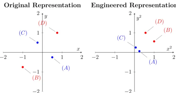
In classification tasks, a useful representation of the data is one which allows for a separation of the points into the required groups. This means that the features need to capture the useful information that correlates closely with the true label. For example, data with featuresxand yand the four data pointsA, B, C, D as seen in Figure 2.1 is not linearly separable in its respective classes (blue vs. red) when using the original features. However representing them as features with valuex2 and
y2results in linearly separable data, making these engineered feature representations
more useful. −2 −1 1 2 −2 −1 1 2 (A) (C) (D) (B) x y
Original Representation
−2 −1 1 2 −2 −1 1 2 (A) (C) (D) (B) x2 y2Engineered Representation
Figure 2.1: Examples of less useful (left) and more useful (right) feature represen-tations.
There are several methods that are generally applied for transforming text into numeric values. One possible representation is bag-of-words with count matrices. In the bag-of-words approach each text is represented by the individual words (tokens) present in it, ignoring the sequence of the text. In a count matrix each row is a single document and each document is represented by a vector containing its feature values. In those vectors each dimension is a specific token and the value is the number of times that token occurs in the specified document. Other representations are also used, such as n-grams, which are similar to bag-of-words, however instead of counting the presence of single words, utilize sequences of n items (which could be words, letters, phonemes, etc.).
This type of transformation has several hindrances. One of them being the amount of time needed, since these representations are manually engineered.
2.3
Neural Networks for Text Representations
A way of circumventing the need for manual feature engineering is to learn that feature representation automatically. A good model architecture for achieving this is a neural network. The universal approximation theorem [5] states that a neural network can approximate any continuous function. This means that any feature representation could be approximated.
2.3.1
Neural Network Basics
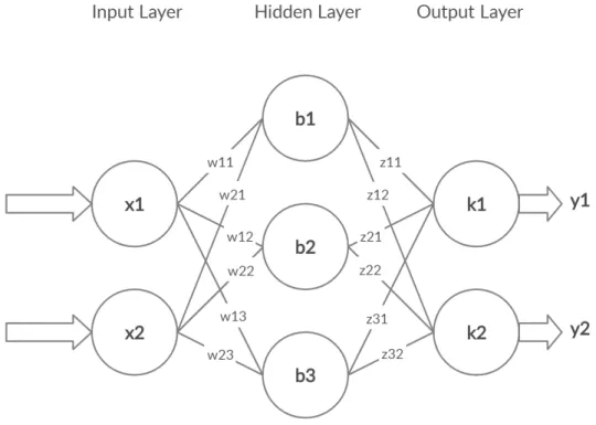
A neural network is a graph-like machine learning model consisting of nodes con-nected by edges as seen in Figure 2.2. The neural network consists of layers of nodes with edges connecting them. There are three types of layers: input, hidden, and output. The first one is where the input data is passed through, while the last layer is the output. These two can be connected by either one or several layers, called hidden layers. The process of producing an output from an input is called a forward pass and consists of calculating the values of each node.
Figure 2.2: An example of a neural network.
For the example given in Figure 2.2, for a data point x1, x2, the values for the
three hidden nodes are respectively:
top node value =b1 +w11·x1 +w21·x2 (2.1) middle node value =b2 +w12·x1 +w22·x2 (2.2)
bottom node value =b3 +w13·x1 +w23·x2 (2.3) These values are then passed through a function, typically a sigmoid or tanh, obtaining the final node valuesh1,h2,h3. This is done to allow for non-linear data relationships and is called an activation function. The values for the output layer are calculated in a similar fashion. That is:
top node value =k1 +z11·h1 +z21·h2 +z31·h3 (2.4) bottom node value =k2 +z12·h1 +z22·h2 +z32·h3 (2.5) These are again passed through an activation function to produce the final predictiony1 andy2.
When training a network the values of the parameters w{ij}, b{i}, k{i} are calculated by a process called backwards propagation. They are usually initialized to random numbers and small changes are applied with each new training data point passed through the network. When a point is passed through the model, the difference between the predicted y values and the true ones is called the loss. The gradient of this loss with respect to each parameter is calculated. Afterwards, a step is taken into the direction of negative gradient in order to minimize the function.
2.3.2
Transformers
Typical neural network architectures for text tasks are based on recurrent neural networks (RNN) [4]. These take into account the sequential nature of the data. The example in Figure 2.3 shows an RNN used for translating a sentence from one language to another.
Figure 2.3: An example of a recurrent neural network [29].
This architecture is split into two parts – an encoder and a decoder – that are simply neural networks. The encoder is fed one word at a time and outputs a hidden state value. This hidden state value, together with the next word are fed through the encoder again. At the end of the input sequence, the hidden state value is fed to a decoder neural network, which produces an output word and a further hidden state value. Those are then fed to the decoder again in order to predict the
next word. An issue with this architecture is that when the word "monde" needs to be output, the word that is being translated is "world", which is passed through the model several steps before. This means that the information needs be retained within the hidden state values for several passes through the model. A way to solve this is to introduce a mechanism that allows the decoder to access the relevant parts from the input sequence. This type of mechanism is called attention [2].
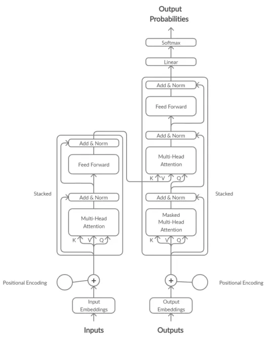
A further development in the field is to simply apply the attention mechanism without recurrence. This new architecture is called a transformer [25].
Figure 2.4: An example of the transformer architecture where both on the left and on the right side, several of the components are stacked on top of each other.
value (V) triplet. In the case of the attention layer, which combines the input sequence and the current output, the key and value come from the input sequence and the query comes from the output. These are combined using the following formula:
attention(Q, V, K) = sof tmax
QKT
√
dk
V (2.6)
wheredk is the number of dimensions of K.
In this formula, the dot productQKT has larger values for keys that are similar to the requested query, the softmax function essentially "picking" the relevant keys. The corresponding values to those keys are then selected. The key-value pairs could be seen as interesting facts found in the input sequence and the query is how they are accessed.
2.4
Transfer Learning
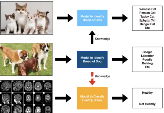
Transfer learning is a machine learning approach which is based on the idea that knowledge gained from learning how to solve problem A could be useful for solving a different problem B in the case they share some similarities. Some similarities in the data type are required – e.g. both problems focusing on images or text data. However, the tasks could be quite different – for example, problem A could be to classify images into ‘cat’ and ‘dog’ categories, whereas problem B could be to identify the exact boundaries of the cat or dog within the image. The knowledge gained most typically consists of the parameter values of the model trained to solve problem A. These can be used as initialisation of the model used for solving problem B instead of starting from an untrained model, making fine-tuning, i.e. the training for solving problem B, much faster.
For example in Figure 2.5 a model meant to identify the breed of dogs in an image can be used to obtain insights that are helpful to identifying the breed of a cat. These insights could consist of the presence of similar animal features within the images such as fur, nose and eyes. However, the same model for identifying the breed of a dog would not be helpful for classifying MRI images and whether they show a healthy brain or not. This is because the extracted features from the first model share no similarities with the second one.
Figure 2.5: An example of transfer learning. The main model is used to identify the breed of dogs. The knowledge gained could be useful for identifying breeds of cats, however, it is probably not useful for identifying healthy brains in MRI images.
There are two main benefits of using transfer learning. The first benefit is that it makes solving the second task much less time consuming, since instead of training the entire model, one would just need to fine tune the initial model. The second benefit is that due to the vast amount of data used to train the initial model, it can significantly increase the performance even without much data at hand for the second task.
2.4.1
BERT
Several high-performing transfer learning models currently available are based on the transformer architecture, such as GPT [20] and BERT [8]. The GPT model uses transformers, which use attention in both directions. However, the task the model is trained on is next word prediction in a left-to-right direction only. Alternatively, BERT has deep bidirectionally due to both the use of the encoding part of the transformer architecture (left part of Figure 2.4) and the language model used for pre-training. The training tasks for BERT are (1) trying to reconstruct a sentence where some words have been masked, and (2) trying to predict whether in sentence pair A-B, sentence B follows sentence A. This allows it to outperform previous models [8] on the General Language Understanding Evaluation (GLUE) leader board [1].
The way BERT encodes an input sequence consists of three levels that are combined as can be seen in Figure 2.6. The first one is the positional encoding
of the word, which refers to its place in the sequence. The second part refers to which document the word appears in, as BERT deals with two documents. The third level is the embedding of each word, where two special tokens are additionally used: one for the beginning of the input (CLS), another for indicating the end of a document (SEP). The model outputs a vector for each of these tokens. Typically, for classification tasks, a linear layer is added on top of the output vector for the CLS token.
Figure 2.6: BERT input representation, where the input is a sum of three levels of embedding [8].
BERT has also shown good results identifying hate speech when applied to English data, as can be seen in [15] and [17].
2.5
Cross-Lingual Representations
Cross-lingual zero-shot learning is a type of transfer learning, where the training language is different to the testing one. This allows for the use of a resource rich language for training. The method relies on the ability of neural network models to learn mappings between different distributions, in this case between the training and the testing language. One approach is to pre-train a model on a multilingual corpus of data. In this set-up, identical subwords in a shared vocabulary can act as anchor points for learning an alignment between languages. Additionally, training on multiple languages at the same time can amplify this effect. Furthermore, due to the ability of deep networks to learn complex patterns, ones that extend beyond simple vocabulary mappings can also be found [22]. Ideally, this would lead to similar representations for texts with similar meanings, independent of the languages. That is, given two text inputs in different languages that have the same meaning (one could be a translation of the other), their representation should be similar.
2.5.1
Multilingual BERT
An extension to BERT is its multilingual version that utilizes the concept discussed above. This extends the base version by training the model on a Wikipedia data set containing 104 different languages. Results using multilingual BERT suggest that there is some alignment between languages that emerges automatically in its
representations. By training on a specific language and testing on a different one, the model has shown some cross-lingual knowledge transfer is occurring for named-entity recognition and part of speech (POS) tagging [19]. Named-named-entity recognition locates and classifies parts of text that represent one of a number of pre-defined categories. For example, in a corpus of text one might be interested in all names of organizations, all locations, etc. Meanwhile, part of speech tagging consists of attempting to mark each word within a text with its corresponding grammatical class, e.g. finding all verbs in a corpus of text. Good results are achieved even for languages in different scripts – e.g. a model trained on Urdu produces 91% accuracy when evaluated on Hindi for POS tagging.
2.6
Data Augmentation
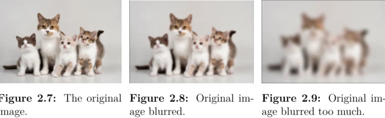
The data augmentation approach is used for creating new data points from existing ones. This is done by slightly changing the feature values of one data point to create a new one. Data augmentation techniques have been applied successfully to image data. One such example is to blur an image available in the data set, as can be seen in Figures 2.8 and 2.9.
Figure 2.7: The original image.
Figure 2.8: Original im-age blurred.
Figure 2.9: Original im-age blurred too much.
One of the most important aspects in the process is the trade-off between di-versity and validity – i.e. the issue of choosing the correct range for the size of the changes. The validity of the label could deteriorate when the changes are too big. As can be seen in Figure 2.9, blurring the image too much makes the object in it unrecognizable. Thus, invalidating the cat label.
Making changes too small, however, diminishes the diversity of the data and therefore its usefulness as a means to create more examples.
With careful selection of the augmentation technique and thresholds for the size of the change, this is a powerful tool for increasing the data size and thus improving the robustness of the model, as by introducing more diverse data, the model will likely perform better on an unseen set.
Creating data augmentation techniques for text is an active area of research. It is not immediately obvious how well-known image augmentation techniques, like stretching and blurring, can be applied to text. Additionally, a particular issue with text augmentation is that even small changes to the data could lead to big changes in the meaning, whereas, images are not as susceptible to change, i.e. changing a
pixel value slightly will not change what the image represents. The relevance of this issue could vary with the specific task at hand, e.g. for a topic classifier recognizing financial documents, changing one word might not affect the topic too much.
Three methods that are explored in this section are: TF-IDF synonym replace-ment, word dropout and back-translation.
2.6.1
TF-IDF Synonym Replacement
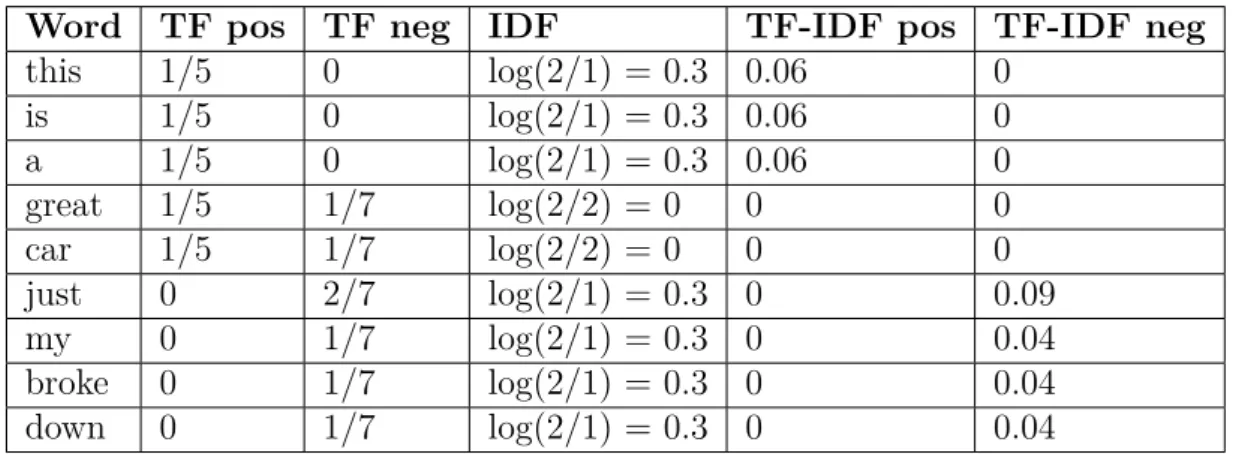
The first method that is utilized is TF-IDF (term frequency inverse document fre-quency) synonym replacement. This method introduces variability by replacing some words with a synonym. In order to not lose the core meaning only the words that do not carry a lot of information should be replaced. Therefore, these are selected based on a TF-IDF score, which is correlated with the importance to the label. It is calculated by multiplying both the term frequency (TF) and the inverse document frequency (IDF), as can been seen:
tf-idf(t, D) = tf ·idf =tf ·logN
df (2.7)
In the equationtf refers to the number of occurrences of termtin all document having labelD;N refers to the amount of documents in the corpus;df refers to the number of documents where the termtappears. Finally, the TF-IDF scores for each label are calculated by multiplying the IDF values with that label’s TF values. That is, for each label, there is a bag of words where each word has a specific TF-IDF score. For example:
Label: ’Positive’
Document One: ’This is a great car.’
Label: ’Negative’
Document One: ’Just great. My car just broke down.’
Word TF pos TF neg IDF TF-IDF pos TF-IDF neg
this 1/5 0 log(2/1) = 0.3 0.06 0 is 1/5 0 log(2/1) = 0.3 0.06 0 a 1/5 0 log(2/1) = 0.3 0.06 0 great 1/5 1/7 log(2/2) = 0 0 0 car 1/5 1/7 log(2/2) = 0 0 0 just 0 2/7 log(2/1) = 0.3 0 0.09 my 0 1/7 log(2/1) = 0.3 0 0.04 broke 0 1/7 log(2/1) = 0.3 0 0.04 down 0 1/7 log(2/1) = 0.3 0 0.04
Table 2.3: Values of TF-IDF scores for example given above.
As can be seen in Table 2.3, terms that appear in both labels (’great’ and ’car’) have scores of 0, whereas terms that appear more frequently in a specific label
(’just’ in ’negative’) have a higher score. This exemplifies the correlation between the TF-IDF score and the importance of a word for a given label.
When a document is selected for augmentation, the TF-IDF scores used are based on the label of the original sentence. A uniform random number is chosen and if the word has a lower TF-IDF score (i.e. indicating the word has low importance), it is changed for a synonym in the augmented document. One advantage of this method is that the document should not lose its meaning since the replacement word has a similar definition to the original one. However, the main concern is for words with more than one definition, as the wrong one could be selected for obtaining the synonym. Examples of good and bad augmentations using this technique can be seen below.
Original Document: My brother is a cool guy
Good Augmentation: My brother is a popular guy
Bad Augmentation: My brother is a cold guy
Original Document: Cinderella had to go to the ball.
Good Augmentation: Cinderella had to go to the dance.
Bad Augmentation: Cinderella had to go to the sphere.
For all examples shown above, the method correctly changes a word for a syn-onym. However, specifically, in the bad augmentation instances, not using the context leads to a change in meaning for the entire document and making it an implausible data point.
2.6.2
Word Dropout
Word dropout is a data augmentation technique where a new document is created by giving every word in the original document the same probability of being removed all together. The new document would then be added to the original data set with the label belonging to the original data point.
An example of word dropout would be:
Original Document:
Sentence: I don’t like Syrian refugees Label: Aggressive
Augmented Document:
Sentence: I don’t like refugees Label Given: Aggressive True Label: Aggressive
In this case, both carry a similar negative connotation. This means that the label would not change, therefore the new data point would be useful for training a model.
However, the main problem that could arise using this method would be to drop a word that carries a much stronger meaning within the sentence. For example:
Original Document:
Sentence: I don’t like Syrian refugees Label: Aggressive
Augmented Document:
Sentence: I like Syrian refugees Label Given: Aggressive
True Label: Non-Aggressive
In this case, the augmented sentence does not retain the aggressive meaning. Since this method gives each augmented sentence the same label as the original version, situations like the example above would not be the most optimal.
2.6.3
Back-Translation
Back-translation consists of translating a sequence into a different language and then translating it back to the original language. The main advantage of back-translation over the previous methods is the fact that it translates the entire sentence, therefore the meaning should not change as much. For example,
Original Document:
Sentence: Yesterday, my dad told me the story of the first time he met my mom.
Intermediate Language: Spanish
Sentence: Yesterday, my dad told me the story of the first time he met my mother.
In this specific case, both sentences mean the same thing. The only change being the word “mom” to “mother”. This change could be seen as too small and providing little variability to the augmented data. In order to increase said variability a more diverse set of intermediate languages could be used. However, back-translation could produce examples that change the original meaning or make less grammatical sense. For example,
Original Document:
Sentence: Yesterday, my dad told me the story of the first time he met my mom.
Intermediate Language: Swedish
Sentence: Yesterday, my dad told me the first time I met my mother.
3
Methods
In this chapter an overview is given of the experimental set-up for the project. The data sets that are used are discussed, along with the annotation guidelines used for each one. The chapter also outlines the training process for obtaining the baselines. Additionally, the specific implementation for the cross-lingual zero-shot and data augmentation approaches are presented. Some experimentation is carried out to observe the effects of training set size and the impact of translating of English training data. The evaluation approach is discussed. Finally, some analyses of the data sets are carried out in order to investigate the cohesive groups present within them.
3.1
Hate Speech Data Sets
Several data sets are used to explore the different aspects of the task at hand. All data sets are tweets that are manually annotated for hate speech. These data sets are balanced between the two classes. The main data set is the HatEval [3] data set, containing tweets in both English (EN) and Spanish (ES). Spanish is used as a proxy for a low resource language and the effect of using English during the training process is explored. These data sets are taken as a basis for the project. Since they belong to the same competition, the data distributions between English and Spanish should be most similar in the gathering process, annotation guidelines and time period. However, additional languages are also used. Those are Arabic (AR) [18], Portuguese (PT) [10] and Indonesian (ID) [13]. For the purpose of a comparison two more English data sets are utilized – Waseem & Hovy (WH) [26] and Founta (F) [11], where tweets are scraped through the Twitter API leading to 4440 balanced training examples in set WH and 5151 balanced training examples in set F.
Minimal modification is done to the data – mentions and URLs are removed, the hashtag sign is dropped leaving each hashtag to be treated as a word. If a letter is repeated 3 or more times, the repetitions are removed.
3.1.1
Annotation Guidelines
As previously mentioned, hate speech has slight differences in its definition. These are reflected in the differences in annotation guidelines for each of the used data sets.
• HatEval1: Hate speech against immigrants is defined as a "message that spreads, incites, promotes or justifies HATRED OR VIOLENCE TOWARDS THE TARGET, or a message that aims at dehumanizing, hurting or intimidat-ing the target" and must have "IMMIGRANTS/REFUGEES as main TAR-GET, or even a single individual, but considered for his/her membership in that category (and NOT for the individual characteristics)". Additionally, hate speech against women is defined as "a text that expresses hating towards women in particular (in the form of insulting, sexual harassment, threats of violence, stereotype, objectification and negation of male responsibility)". An important note is made that this data set does not label hate speech against any target other than immigrants/refugees or women as hate speech. In other words. it is only concerned with those two target groups.
• Founta: "Language used to express hatred towards a targeted individual or group, or is intended to be derogatory, to humiliate, or to insult the members of the group, on the basis of attributes such as race, religion, ethnic origin, sexual orientation, disability, or gender". [11] As can be seen a wider range of targets is considered. In this data set, the annotators are asked to label each tweet with one of the following categories: normal, spam, abusive, and hateful, making an explicit distinction between abusive language and hate speech. • Waseem & Hovy [26]: This data set gives an eleven-point guideline for what
is considered hate speech, which is mainly centered around using sexist/racial slurs, attacking/seeking to silence/criticizing a minority or defending such be-haviour. Two further points take into account the specific Twitter nature of the data. Tweets supporting problematic hashtags are labeled as hate speech. Additionally, ambiguous tweets from users with offensive screen names are also considered hate speech. This data set focuses on sexism and racism as the only categories of interest.
• Indonesian[13] : In order to arrive at a definition of hate speech a focus group discussion is conducted. It is concluded that hate speech has a particular tar-get, category and level. For targets, as in the previously mentioned definitions, both individuals and groups are considered. However, the categories have a wider range with religion, race/ethnicity, physical disability, gender, sexual orientation all being considered. The label is further split into levels, however all levels are considered as hate speech examples.
• Arabic : "Hate speech tweets are those instances that: (a) contain an abu-sive language, (b) dedicate the offenabu-sive, insulting, aggresabu-sive speech towards a specific person or a group of people and (c) demean or dehumanize that per-son or that group of people based on their descriptive identity (race, gender, religion, disability, skin color, belief)." [18] Similarly to Founta, the label is split into normal, abusive and hate.
• Portuguese : “Hate speech is language that attacks or diminishes, that in-cites violence or hate against groups, based on specific characteristics such as physical appearance, religion, descent, national or ethnic origin, sexual
entation, gender identity or other, and it can occur with different linguistic styles, even in subtle forms or when humour is used.” [10]
3.2
Baseline
Two models are used as a baseline for determining multilingual BERT’s ability to detect hate speech – a model trained on all available Spanish tweets (Spanish base) and a model trained on the same size of English tweets (English base). These tweets are taken from the HatEval data set that contains both English and Spanish data annotated with similar guidelines. The data is balanced where 50% of the tweets are labeled hate speech.
The data is split into three data sets – training, validation and testing. The training data is passed through the model for finding the weights. The validation set is used to calculate the performance of the trained model for each hyper-parameter set, in order to determine the best one. The testing set is used to calculate the per-formance of the final model. Separate validation and testing data sets are needed to avoid over-estimating the performance. Since the hyper-parameters are selected based on the performance on the validation set those could be over-fit to the val-idation data. Therefore, to predict real-world performance a completely held out (testing) set is needed – i.e. one that has not been used in any stage of the hyper-parameter tuning process.
Spanish base utilizes all available data in HatEval, which consists of 3600 tweets. This is the number used for training both the Spanish base and the English base models. As English base is evaluated for cross-lingual zero-shot learning, the per-formance of the model on its own test set is used as a baseline for the comparison.
The base models are also used for performing a hyper-parameter search, where the hyper-parameters that are found to have the best performance are used for all following models. Several hyper-parameters are important when using BERT.
The first hyper-parameter to be explored is the learning rate which is central to any neural network. This determines the size of the change in the model’s param-eters at each step. A small learning rate makes the changes too small, making the converging of the model slower. A large learning rate could lead to the impossibility of converging as the big changes in the parameters can ’overshoot’ the optimum. For BERT there is a recommended range of learning rates that are explored: 5×10⁻⁵, 3×10⁻⁵, 2×10⁻⁵.
In order to reduce the chance of over-fitting (i.e. learning the training data instead of the general patterns) dropout in both the hidden layer and the attention layer is used [24]. This is controlled by the dropout rate parameter. It determines a percentage of random connections between nodes that are ignored during training. The default dropout rate for the BERT model is 10 percent. Several values are ex-plored to find any improvement in the model’s performance. Initially, one parameter at a time is tested to provide a relative range that is used to perform a grid search of both parameters at the same time.
number of passes through the training data that are needed to find the optimal weights. Since neural networks change their parameters based on a subset of the data at each step of the training process, this means that further data can cause the network to "unlearn" previous patterns – i.e. change the parameters in the opposite direction. Validation accuracy after each epoch is used to determine the correct number. Once the validation accuracy stops increasing with additional epochs the model is stable and further passes through the data do not lead to improvements.
Both baselines are trained and tested 10 times in order to obtain a range for the performance and a sense for the stability of the models. This is done for all models used in this work.
3.3
Cross-Lingual Zero-Shot Learning
The English base model’s performance is evaluated on a Spanish test set to assess the possibility for cross-lingual zero-shot learning.
Additionally, several other Twitter data sets annotated for hate speech are used for testing both the English base and the Spanish base model to assess the performance on other languages.
Two additional English Twitter data sources are used for training models. Those models are evaluated on a test set from each of the three available English sources. This offers a baseline to put all the previous results in context, as these models should show minimal drop in performance, due to no cross-lingual learning being needed. There are several possible sources of differences in these data sets: the time period they were collected in – which could lead to difference in the topics discussed, annotation – which could introduce differences in bias, and the collection process – i.e. how is that subset of tweets selected (while some data sets are randomly extracted, others are targeted by searching for specific terms). For a model to be useful for the general detection of hate speech, these differences should be negligible.
3.4
Effects of Training Set Size on Performance
To explore the effect of small training sets on performance, the accuracy of models trained on a range of sizes of the proxy language (Spanish) is obtained. This provides a sense of how performance depends on size and when the scarcity of data becomes a significant issue. A series of sizes are explored – 250, 500, 1000, 1500, 2000, 2500, and 3000 tweets. All sets are balanced and the same hyper-parameters are used as the optimal ones found for the base model that is trained on 3600 Spanish tweets. The expected trend is reduced performance with reduced size.
3.5
Data Augmentation
In this project, data augmentation is applied to increase the size of a data set by adding additional tweets to the already existing ones. As already mentioned, those
tweets are generated by three different methods. Three different data sizes (250, 1000, and 2000) are used as examples of very small, medium and relatively large data sets. This shows whether the data augmentation methods lead to improvements for a specific size of data. Each of the three reduced data sets are increased in size in steps to follow the series 250, 1000, 2000 and 3600.
3.5.1
TF-IDF Synonym Replacement
The first data augmentation technique that is implemented is TF-IDF synonym replacement. The implementation of the method is based on previous work [28]. As previously mentioned this augmentation relies on substituting a word for its synonym. In order to obtain a synonym the Open Multilingual Wordnet repository [12] is used. A list of synonyms is extracted by getting all possible translations in English and for each of those translations getting all possible translations back to Spanish. A random word from that list is then selected.
In order to decide which words should be replaced a random number between 0 and 1 is assigned to each word contained within it. If this number is less than the threshold calculated by equation 3.1 the word is replaced by a synonym. This threshold is normalized for each tweet using the mean and maximum TF-IDF score of the entire tweet.
threshold=min(1, constant· maxScore−wordScore
meanScore ) (3.1)
The constant is the parameter that has to be tuned in order to find which value works the best.
3.5.2
Word Dropout
The second data augmentation method that is used is word dropout. This approach is based on previous works as seen in [28] and [27]. It is implemented by selecting a random tweet to be augmented and assigning a random number between 0 and 1 to each of its words. If this number is less than a certain threshold, said word is dropped entirely from the augmented tweet. The main parameter that has to be tuned in this specific method is the threshold.
3.5.3
Back-Translation
The final data augmentation method is back-translation. This is based on previous work described in [28]. It translates each tweet into a random language and then translates it back. The process is done through the Google API and the intermedi-ate language is chosen at random from a list of 106 different ones. As all languages available through the API have the same probability of being chosen as a middle language, the dependency on which one is used is reduced. This also allows for mul-tiple translations, i.e. augmentations, from a single tweet. The linguistic proximity between the original and middle languages could influence the quality of the data
augmentation and can be seen as a hyper-parameter for the technique. However, this effect is not been explored in the current project.
3.6
Translation of English Training Data
A further method for obtaining a large training data set is to translate a data set in a resource rich language to the required language. In this particular case the HatEval English training data is translated to Spanish, Arabic, Portuguese and Indonesian. The Google API is used to obtain a single translation. This introduces some further variability which is governed by how well the Google API performs in translating between a particular pair of languages.
3.7
Evaluation
The evaluation follows the standard protocol for this type of task. As can be seen in [3] the metrics that are used are accuracy (ACC), precision (PRC), recall (RCL) and F1 score (F1).
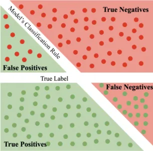
In a classification task with two classes, where one is positive and one is negative, there are four types of data points: true positives, true negatives, false positives and false negatives, as can be seen in Figure 3.1. For this specific project the positive class can be seen as the examples containing hate speech.
Figure 3.1: Example of true positive and negative elements versus selected positives and negatives. The green and red points refer to positive and negative true labels, respectively. While the green and red backgrounds refer to what the model considers positive and negative, respectively.
Based on said counts, the metrics are calculated as follows:
ACC = T P +T N
P RC = T P T P +F P (3.3) RCL = T P T P +F N (3.4) F1 = 2· P RC·RCL P RC +RCL = 2·T P 2·T P +F P +F N (3.5)
As the data sets are balanced, accuracy is a good primary measurement. To as-sess any instability due to the random initialisation of the models each one is trained and tested 10 times, and the average of each metric with its standard deviation is calculated.
For any hyper-parameter or data augmentation threshold search a validation set is used for evaluation, whereas the final results are calculated on a further held-out test set. The validation and test sets for all experiments are of size 400 tweets with 200 hate speech and 200 non-hate speech examples.
3.8
Data Sets Analyses
Some further investigation into the data is performed in order to give a broader picture of all aspects of the task. Clustering and classification analyses are used for detecting any possible groups within the data that could hinder the model. This is done in order to examine whether a different label produces similar results or hate speech is intrinsically hard to model.
3.8.1
Clustering
As previously mentioned in section 2.1.1, clustering is used for discovering groups of similar data. In this project the clustering model applied is k-means. As k-means finds local optima it is dependent on initialization. To get a stable performance ten random initializations are used.
Two data representation are used – TF-IDF and BERT vectorization. As dis-cussed in section 2.2, count matrices are used. For TF-IDF a token is considered to be each word present and the count matrix is normalized by the TF-IDF scores. Whereas for the BERT approach, the BERT tokenizer (based on WordPiece) is used to generate the tokens. This tokenizer can split unknown or longer words into multiple sub-words. A double hashtag in the token represents that this is not the beginning of a word, as can be seen:
Original Document:
Here is the sentence I want embeddings for.
Tokens:
’here’, ’is’, ’the’, ’sentence’, ’i’, ’want’, ’em’, ’##bed’, ’##ding’, ’##s’, ’for’, ’.’
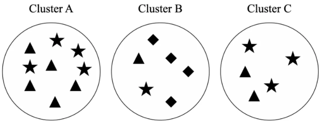
For evaluation of how well the clusters found align with the classes of interest (as defined by the labels) two metrics are used – the purity and inverse purity. These are calculated using:
purity= 1 N X k max j |wk∩cj| (3.6)
In the formula above wk refers to the data points having label k and cj refers
to the data points in clusterj. In order to calculate the inverse purity thewk refers
to the cluster andcj refers to the data point label. An example of these calculations
is given in Figure 3.2.
Figure 3.2: Purity and inverse purity calculation for the three clusters above. Majority class for each cluster: cluster A: N, 5; cluster B: , 4; cluster C: F, 3. Purity = 201(5+4+3) ≈0.6. Majority label for each class: N: cluster A, 5: cluster B, 4F: cluster A, 4. Inverse purity = 201(5+4+4) ≈ 0.65.
Furthermore, in order to investigate the contents of each cluster the top 10 most descriptive tokens are obtained. Each cluster is represented by a centroid, which is a vector with a dimensionality equal to the number of available tokens. Each dimension/token has a corresponding weight. The tokens corresponding to the highest weights are selected as the most descriptive ones.
In the current project the groups of interest are hate speech vs non-hate speech. Additionally, clustering is applied in order to determine whether the three different English training data sets are distinct enough to form individual groups.
3.8.1.1 Clustering for Hate Speech
A clustering algorithm is applied on both the English HatEval and Spanish HatEval data sets. This is done in order investigate whether there is a strong signal in the data that can be used to split into cohesive groups. Ideally the resulting clusters would show a correlation between the clusters found and the hate speech vs. non-hate speech label. This would mean that the vocabulary found in each class is distinct enough.
3.8.1.2 Clustering English Training Data Sets
A clustering algorithm is applied on an amalgamation of all three English training data sets, i.e. all three data sets are joined into a single one. The label used for this investigation is the training data set source. A correlation between the cluster and the label would mean that a data source uses vocabulary distinct from the other sources. This could happen if one of the data sources focuses on completely different events, e.g. discussing the American elections versus the Syrian refugee crisis in Europe.
A more detailed view of the correlation between clusters and labels of interest can be obtained by producing data distributions by clusters. This is done by plotting the percentage of data falling within each cluster for each label value. For example, in the case when data sources are explored, the percentage of data coming from Source 1 and falling in cluster 1, 2 and 3 respectively, is calculated. Similarly, this is calculated for Source 2 and 3. Both data source and hate speech labels are explored, to evaluate their correlation with 3 and 2 clusters respectively. If clusters perfectly correspond to labels, the plots are expected to approximate the ones presented in Figure 3.3, i.e. each of the groups should have 100 percent of its data in its own distinct cluster. 0 1 2 3 4 0.2 0.4 0.6 0.8 1 Cluster number % of p oin ts in cluster
Data Source
Source 1 Source 2 Source 3
0 1 2 3 0.2 0.4 0.6 0.8 1 Cluster number
Hate Speech Label
Hate Non-Hate
Figure 3.3: Distribution of data compared to labels when perfect correlation is observed.
3.8.2
Classifying English Training Data Sets
A further investigation into a possible dissimilarity between the different English data sources is done. A pre-trained Multilingual BERT classifier is fine tuned on the same data set as Section 3.8.1.2, where all the English training data sets have been joined together. If the classifier shows good performance it could point to
the model being able to learn particularities of the data, rather than the general patterns of hate speech.
For evaluation the accuracy and a confusion matrix are used. The latter shows the number of data points that are labeled by the model as a specific class vs the true label of those data points. An example of this for a case with two classes where one is positive and the other is negative can be seen in Table 3.1
True Label
Positive Negative Predicted Label Positive True Positive False Positive
Negative False Negative True Negative
Table 3.1: A confusion matrix with two classes
The training and testing is repeated ten times in order to obtain mean and standard deviation for each of the evaluation matrices in question.
4
Results
The current section presents the results for both explored methods. Cross-lingual zero-shot learning shows better results than a random classifier, while still exhibiting a substantial drop from the baseline. Meanwhile, two of the data augmentation techniques show improvements when used on the smaller data set sizes.
For these models, the main metric used for evaluation – the accuracy – is relatively stable with standard deviations in the range 1% - 4%. However, the other three metrics show more variability with standard deviations going all the way up to 11.57%.
The additional data set exploration experiments show no substantial topic dif-ferences in either the hate vs non-hate speech groups or between the three different English data sets. However, the classification experiment suggest the BERT model might be able to learn data set particularities rather than general hate speech pat-terns.
4.1
Baseline
As previously mentioned, two baselines are trained using 3600 English and 3600 Spanish tweets respectively. A hyper-parameter search is performed as a first step in order to determine optimal values.
Figure 4.1: Spanish base grid search. Darkest green indicates highest accuracy value – 83.73.
Figure 4.2: English base grid search. Darkest green indicates highest accuracy value – 80.75.
perfor-mance for both the English and the Spanish base models is 2×10⁻⁵. Performance
on the validation set seems to reach its peak after 10-15 epochs while not dropping for more epochs. As multiple models are trained and tested, in order to accommo-date any models that need more epochs to reach their peak some margin is added. Models are evaluated based on performance after they are trained for 30 epochs. For dropout rate a grid search is performed, testing each set of values. The results are shown in Figures 4.1 and 4.2 where it can be seen that the best set for both models is hidden layer dropout rate of 0.25 and attention layer dropout rate of 0.20. The results on the testing sets are shown in Table 4.1. The English base results are comparable to previous work on the same data set as seen in [15], where the accuracy obtained is 74.8% using the base English BERT model.
Train Test ACC RCL PRC F1 EN EN 73.9 66.6 78.1 71.65
ES ES 80.67 80.55 80.83 80.62
Table 4.1: Performance of the English Base (EN) and Spanish Base (ES).
4.2
Cross-Lingual Zero-Shot Learning
As mentioned in Section 3.3, both baselines are tested for performance on all other available languages. A completely random classifier with two classes and balanced data would result in an accuracy of 50%. As can be seen from Table 4.2, most of the cross-lingual zero-shot experiments have an accuracy above a random classifier. However, there is a significant drop from the baselines (i.e. trained and tested on English and trained and tested on Spanish).
Train Test ACC RCL PRC F1 EN EN 73.9 66.6 78.1 71.65 EN ES 56.03 ↓ 26.05 66.15 36.52 EN AR 57.65 ↓ 23.0 76.06 34.64 EN ID 51.58 ↓ 7.55 62.24 13.22 EN PT 55.55 ↓ 17.35 74.04 27.73 ES ES 80.67 80.55 80.83 80.62 ES EN 54.18 ↓ 19.55 64.16 29.44 ES AR 50.72 ↓ 8.25 55.82 14.12 ES ID 51.52 ↓ 9.3 61.42 15.84 ES PT 60.35 ↓ 36.45 70.04 47.69
Table 4.2: Performance of English and Spanish base on other languages. Baselines with no cross-lingual learning are shown in gray.
The base English model, when evaluated on the Spanish test data set shows a significant drop in performance of 16%. This trend is also observed for the other test languages – summarized in Table 4.2. The worst performance is shown by the base Spanish model evaluated on Arabic and best performance is shown by the same
model evaluated on Portuguese. None of the cross-lingual zero-shot evaluations show an accuracy above 60% independent of the original model’s performance on its own test set – i.e. even though the base Spanish model has almost 10% higher accuracy score on its own data set, the drop in performance is comparable for both the English base and Spanish base models. Some correlation between performance and language group is observed (e.g. Spanish on Portuguese performs better than Spanish on Arabic), however, these differences seem to be dominated by the general drop for all languages. It can also be observed that a drop in recall is much more evident than a drop in precision, likely driving the drop in accuracy. This points to much more lenient decision-making on different languages, marking less examples as hate speech.
The results from all three available English data sets tested on each other can be seen in Table 4.3. The two additional data sets show a higher accuracy on their own testing data, however a similar drop into the 60s is observed when testing on other English test sets.
Train Test ACC RCL PRC F1 HatEval HatEval 73.9 66.6 78.1 71.65 HatEval WH 57.75 ↓ 28.18 68.81 39.58 HatEval F 57.87 ↓ 22.83 76.46 34.87 WH WH 82.55 79.97 84.38 82.05 WH HatEval 60.08 ↓ 57.85 61.09 58.92 WH F 62.11 ↓ 37.98 74.00 49.35 F F 81.64 78.30 84.07 80.99 F HatEval 59.25 ↓ 75.05 57.13 64.75 F WH 66.13 ↓ 68.81 65.68 66.84
Table 4.3: Performance of different English models. Baselines on own test sets are shown in gray. WH refers to [26], F refers to [11] and HatEval refers to [3].
Since both Waseem & Hovy and Founta perform better on their respective held-out test sets, both models are tested on all other available languages to test their cross-lingual zero-shot performance. The results can be seen in Tables 4.4 and 4.5 for Waseem & Hovy and Founta, respectively. Waseem & Hovy shows a similar accuracy to HatEval, however the F1 score is higher mainly due to more balanced precision and recall scores. Founta shows accuracy improvement for all languages other than Spanish, as well as a substantial improvement in F1 scores.
Train Test ACC RCL PRC F1 WH WH 82.55 79.97 84.38 82.05 WH ES 53.52 43.15 54.58 47.6 WH AR 55.62 34.6 60.73 41.66 WH ID 53.25 17.3 62.09 26.48 WH PT 56.75 34.8 62.3 44.23
Table 4.4: Performance of Waseen & Hovy data set on other languages. Baseline with no cross-lingual learning are shown in gray.
Train Test ACC RCL PRC F1 F F 81.64 78.30 84.07 80.99 F ES 56.5 ↓ 51.7 57.09 54.03 F AR 60.25 ↓ 51.85 62.41 56.02 F ID 59.38 ↓ 58.35 59.7 58.87 F PT 63.5 ↓ 69.1 62.22 65.36
Table 4.5: Performance of Founta data set on other languages. Baseline with no cross-lingual learning are shown in gray.
4.3
Effects of Training Set Size on Performance
As stated in Section 3.4, the effects of training set size on performance are evaluated. This is done in order to evaluate when resources become too scarce and start sub-stantially affecting the accuracy. This relationship can be seen in Figure 4.3. When data set size is in the thousands accuracy does not seem to depend as much on size. In that region accuracy increases 5.65% when size is increased from 1000 to 3600 (3.6 times). However, when sizes are in t
![Figure 2.3: An example of a recurrent neural network [29].](https://thumb-us.123doks.com/thumbv2/123dok_us/792757.2600213/22.892.156.734.783.948/figure-example-recurrent-neural-network.webp)
![Figure 2.6: BERT input representation, where the input is a sum of three levels of embedding [8].](https://thumb-us.123doks.com/thumbv2/123dok_us/792757.2600213/26.892.178.697.316.473/figure-bert-input-representation-input-sum-levels-embedding.webp)