paircompviz: An R Package for Visualization of Multiple Pairwise Comparison Test Results

(1)

Multiple Pairwise Comparison Test Results

Michal Burda University of Ostrava

Abstract

The aim of this paper is to describe an R package for visualization of the results of multiple pairwise comparison tests. Having data that capture some treatments, multiple comparisons test for differences between all pairs of them. Thepaircompvizpackage pro-vides a function for visualization of such results in Hasse diagram, a graph with significant differences as directed edges between vertices representing the treatments.

Keywords: multiple, pairwise, comparison, test, visualization, Hasse diagram, R.

> library(paircompviz)

1. Introduction

Visualization is an important tool for exploration, analysis and presentation of data. A clear and vivid figure or diagram can improve significantly the readibility of the presented facts. In this paper, an implementation of a novel technique for visualization of multiple comparison test results is presented. Multiple comparison tests (or pairwise tests) occur in testing for differences between all pairs of k treatments (Hsu 1996). It is a common fact that for k

treatments, a batch of k₂

= k(k₂−1) tests has to be performed to compare all pairs.

Typically, the pairwise comparison tests are performed on treatment means, but they may be also applied on other statistics such as variances, quantiles, or proportions.

Multiple comparison procedure usually results in a triangular matrixM of p-values, where the cellmij of matrixMhas p-value of test for difference between treatmentsiandj. Comparisons with p-value below some given threshold α (usually α = 0.05) are considered statistically significant.

Even for as small number of treatments (e.g. k= 5), it is rather inconvenient to perceive the results directly. An appropriate visualization may significantly improve the understandability. A common approach for visualization of multiple comparisons is a line or letter diagram (Gramm, Guo, H¨uffner, Niedermeier, Piepho, and Schmid 2007; Ennis, Fayle, and Ennis 2009).

The main ideas of these diagrams are briefly described on the following example. Assume treatments T1, . . . , T5 such that T1 and T5 is the only significantly different pair. The line

(2)

T1 T2 T3 T4 T5

(a) Line diagram

T1 T2 T3 T4 T5

a a a a b b b b

(b) Letter diagram

Figure 1: Diagrams of treatmentsT1, . . . , T5 such that only treatments T1 andT5 are

signifi-cantly different, i.e. treatments underlined with the same line or sharing a common letter are not (significantly) different.

T1 T2 T3 T4 T5

a a

b b

c c c

d d d

Figure 2: An example of letter diagram for which the corresponding line diagram can not be constructed.

(e.g. mean) into increasing order. (2) Draw a line under all largest groups of treatments such that no pair of treatments in that group is significantly different. Since there are two groups of pairwise-non-significant treatments, the resulting line diagram contains two lines – see Figure1(a).

Some authors (e.g. Piepho(2000)) prefer to use letters instead of lines, because it is sometimes not possible to represent all statements of significance by a diagram with non-interrupted lines. The general idea is to replace each line of the line diagram with a letter – see letter diagram in Figure1(b) that is equivalent to line diagram in Figure1(a).

Consider now the only significant treatments be pairs (T1, T5),(T1, T3),(T2, T4). A

correspond-ing letter diagram is depicted in Figure2. For that case, a line diagram does not exist since it is not possible to draw all lines without interrupting them (Piepho 2000;Grammet al.2007). Letter diagrams can be quite complicated even for such simple setting as in the previous example. Since letter diagrams visualize groups of non-significant treatments, it may be sometimes hard to immediately determine the significantly different pairs of treatments. Therefore the package paircompviz, a novel Rimplementation of the visualization technique based onHasse diagrams, is presented in this paper. Unlike letter diagrams, Hasse diagrams explicitly depict the significant pairs in an easy-understandable way. Moreover, additional visual information can be introduced within the diagrams, such as treatment means, sample sizes or p-values. The author believes that Hasse diagrams provide a vivid and easily under-standable alternative to letter diagrams for visualization of the all-pairwise comparison test results.

2. Hasse Diagrams

Before describing the proposed visualization technique, some important notions have to be defined.

(3)

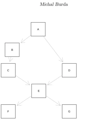
A B C D E F G H

Figure 3: An illustrative Hasse diagram (see the example in section 2).

A partial order is a binary relation Q ⊆ P ×P, which is reflexive, antisymmetric, and transitive. Apartially ordered set is a setP equipped with a partial order relationQ. Hasse diagram is a simple picture of a finite partially ordered set. It is a graph with each member of a set P being represented as a vertex. A directed edge is drawn downwards from vertex y to vertex x if and only if (x, y) ∈ Q, x 6= y, and there is no such z that (x, z) ∈ Q∧ (z, y) ∈ Q. Each edge must be connected to exactly two vertices: its two endpoints. In other words, x, y∈Q iff y is positioned above x and there exists a path from

y tox.

Example. Consider Hasse diagram in Fig.3. As can be seen, nodeAis greater than all other nodes except H, because there exists a path from A to any other node except H. Nodes

C and D are incomparable, although they are both greater than E, F and G. Node H is incomparable with any other node. The whole partial order relation is: n(B, A), (C, B),

(C, A),(D, A),(E, C),(E, B),(E, A),(E, D), (F, E),(F, C), (F, B),(F, A),(F, D), (G, E),

(G, C),(G, B),(G, A),(G, D),(A, A),(B, B),(C, C),(D, D),(E, E),(F, F),(G, G),(H, H)o.

3. Visualization of All-Pairwise Comparison Tests

Consider now an all-pairwise comparison testτ of statisticψonktreatmentsT1, . . . , Tk. Let

ψ(Ti) denote a value of statisticψ on treatmentTi. For instance, if ψwould be a mean, then

ψ(Ti) would denote the mean value of treatment Ti. Let τ(Ti, Tj) < α denote statistically significant difference between treatments Ti and Tj at the significance level α (e.g. τ could be a two sample Student’st–test).

(4)

If a relation H = (Ti, Tj) |i=j∨ ψ(Ti)< ψ(Tj) ∧ τ(Ti, Tj)< α (1) is a partial order on{T1, . . . , Tk}, it can be depicted as a Hasse diagram.

Functionpaircompof thepaircompvizpackage is intended to create Hasse diagrams from the result H of multiple comparisons. Graph rendering is performed with theRgraphvizpackage (Gentry, Long, Gentleman, Falcon, Hahne, Sarkar, and Hansen 2013).

As an example, consider a cholesterol dataset from the multcomp package by Hothorn, Bretz, and Westfall(2008a). It contains measures of cholesterol response (cholesterol$response) to 5 treatments (cholesterol$trt). > library(multcomp) > head(cholesterol) trt response 1 1time 3.8612 2 1time 10.3868 3 1time 5.9059 4 1time 3.0609 5 1time 7.7204 6 1time 2.7139

Let us perform a pairwise Student’st test onresponsegrouped by trt:

> pairwise.t.test(cholesterol$response, cholesterol$trt)

Pairwise comparisons using t tests with pooled SD data: cholesterol$response and cholesterol$trt

1time 2times 4times drugD

2times 0.06400 - -

-4times 0.00023 0.06870 -

-drugD 2.8e07 0.00053 0.06870

-drugE 1.1e-12 2.1e-09 2.7e-06 0.00139 P value adjustment method: holm

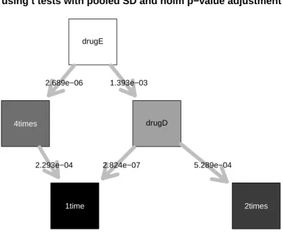
We can see many statistically significant results (for significance level α= 0.05), however, it is not immediately clear, which group response is greater than other etc. Let us depict the results in a Hasse diagram (see Fig.4):

> paircomp(obj=cholesterol$response, grouping=cholesterol$trt, test="t")

(5)

1time 2times 4times drugD

drugE

2.293e−04 2.824e−07 5.289e−04

2.689e−06 1.393e−03

Pairwise comparisons on cholesterol$response by cholesterol$trt using t tests with pooled SD and holm p−value adjustment

Figure 4: Hasse diagram from pairwiset test on thecholesterol data

Thetestargument specifies the type of pairwise tests. Possible values are: "t","prop", and

"wilcox", forttest, proportion test and Wilcoxon rank sum test, respectively. See alsostats

package functions pairwise.t.test,pairwise.prop.test and pairwise.wilcox.testfor details.

Other function arguments are: level, main, visualize, result, draw and compress. The last argument is described separately in section 3.2.

Thelevelargument is for setting the significance thresholdα (default is 0.05),mainspecifies the diagram title. Ifresult is TRUE, the test statistics are also returned from the paircomp

function. Diagram drawing can be disabled by settingdraw toFALSE.

The visualize argument is a vector of string flags that enable drawing of some additional graphical information into the diagram. The meaning of the flags depends on the type of the test being used (t test, Wilcoxon test, or proportion test). If "position" is present in the vector, the vertices background color is derived from mean, median, or proportion, respectively, "size" enables vertices sizes to correspond to sample sizes, and finally, the presence of"pvalue"enables p-value labels along with edges as well as varying edge thickness corresponding to p-value of the comparison test.

There may be also other arguments passed to the paircomp function. They are transpar-ently forwarded to the underlying pairwise comparison tests functions (pairwise.t.test,

pairwise.prop.test, or pairwise.wilcox.test). For instance, a different p-value adjust-ment method may be required. For that, ap.adjust.methodargument exists in the under-lying functions:

> paircomp(InsectSprays$count, InsectSprays$spray, test="t",

(6)

See help pages for more details.

3.1. Displaying Pairwise Comparisons Provided by the multcomp Package Another method for pairwise comparisons is provided by the multcomp package (Hothorn

et al. 2008a). Moreover, that package allows to depict box-plots enriched withcompact letter display that was discussed in section 1. The multcomp package provides Tukey’s test for multiple comparisons by theglhtfunction. Results from that function may also be passed to

paircompin order to generate a Hasse diagram from it. An example on car90dataset from

therpartpackage (Therneau, Atkinson, and Ripley 2013) follows:

> library(rpart) # for car90 dataset

> library(multcomp) # for glht() and cld() functions

> aovR <- aov(Price ~ Type, data = car90)

> glhtR <- glht(aovR, linfct = mcp(Type = "Tukey"))

> paircomp(glhtR, compress=FALSE)

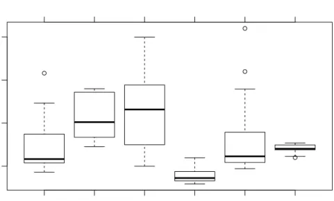
Compare Hasse diagram in Fig.5with compact letter display in Fig.6:

> cldR <- cld(glhtR)

> par(mar=c(4, 3, 5, 1))

> plot(cldR)

3.2. Edge Compression

Sometimes, the pairwise comparison tests may yield in such bipartite setting that each pair of nodes of some two node subsets is inter-connected (without any intra-edge between nodes of the same subset).

More specifically, letU,V be non-empty sets of vertices,U∪V ⊆ {T1, T2, . . . , Tn},U∩V =∅, such that for eachu ∈U and v ∈V there exists an edge fromu to v. (The number of such edges equals|U| · |V|.) Starting from|U|>2 and|V|>2, the Hasse diagram may become too complicated and hence confusing. Therefore, a compress argument exists in the paircomp

function that enables “compression” of the edges in such a way that a new “dot” node w is introduced and |U| · |V|edges between sets U and V are replaced with |U|+|V|edges from set U to node wand from node wto set V. See figures 7and 8 for resulting diagrams of the following commands:

+ compress=FALSE)

+ compress=TRUE)

4. Notes on Partial Orderness of Multiple Comparisons

The ability of visualizing all-pairwise comparisons in Hasse diagram relies on whether relation

(7)

Compact Large Medium Small Sporty Van 1.632e−02 5.104e−05

5.728e−04 5.718e−03 5.536e−03

9.637e−04

Pairwise comparisons on Price by Type using two sided Tukey test

Figure 5: Hasse diagram from results of the glht function. Corresponding compact letter display is depicted in Fig.6 below.

● ●

●

Compact Large Medium Small Sporty Van

10000 20000 30000 40000 Type Pr ice b b c c a b a b

Figure 6: Box-plot with compact letter display on top, as generated by themultcomppackage. Please compare with the equivalent Hasse diagram in Fig.5.

(8)

A B

C

D E

F

8.720e−10

6.872e−07 4.036e−09 4.192e−129.702e−082.479e−081.371e−101.191e−10 3.584e−09

Pairwise comparisons on InsectSprays$count by InsectSprays$spray using t tests with pooled SD and holm p−value adjustment

Figure 7: Hasse diagram without compressed edges, i.e. generated by functionpaircompwith argumentcompress=FALSE(compare with Fig. 8)

A B

C D E

F

.

Pairwise comparisons on InsectSprays$count by InsectSprays$spray using t tests with pooled SD and holm p−value adjustment

Figure 8: Hasse diagram with edges being compressed by introducing a “dot” edge, i.e. gen-erated by functionpaircompwith argument compress=TRUE (compare with Fig.8)

(9)

H(see equation1) is a partial order. Generally, it is not true for all possible data. For instance, consider artificial data,brokentrans1, that is a part of the paircompvizpackage:

> data("brokentrans")

> tapply(brokentrans$x, brokentrans$g, mean)

1 2 3

8.240625 42.215852 95.239536

> pairwise.t.test(brokentrans$x, brokentrans$g, pool.sd=FALSE)

Pairwise comparisons using t tests with non-pooled SD data: brokentrans$x and brokentrans$g

1 2

2 1.3e11

-3 -3.5e-09 -3.-3e-10

P value adjustment method: holm

Forlevelargument set toα= 10−9, we obtain H={(1,2),(2,3),(1,1),(2,2),(3,3)}, which is clearly not a partial order because of broken transitivity between 1 and 3. Thepaircomp

function would stop with an error, in this case.

Although there do theoretically exist data such that its pairwise comparisons does not form a partial order and thus are not viewable in Hasse diagrams, it is rational to estimate the frequency of such settings in real life. For that purpose, a simple experiment was performed by utilizing datasets from packagescluster(Maechler, Rousseeuw, Struyf, Hubert, and Hornik 2012),coin(Hothorn, Hornik, van de Wiel, and Zeileis 2008b),datasets(R Core Team 2013),

lattice(Sarkar 2008), MASS(Venables and Ripley 2002), multcomp (Hothorn et al.2008a),

party,reshape2 (Wickham 2007),rpart (Therneau et al. 2013), strucchange(Zeileis, Leisch,

Hornik, and Kleiber 2002), survival (Therneau 2012) and vcd (Meyer, Zeileis, and Hornik 2012).

From that packages, all datasets were added to the experiment, if they contained a factor column with at least 3 levels. For all combinations of factor and numeric columns, various multiple comparison tests were performed and the cases with broken transitivity condition counted. Table 1 summarizes the frequencies of the numbers of grouping levels of datasets used in the experiment.

As can be seen in table2, among 3150 different test cases, only 3 of them, all made with the Wilcoxon rank sum test, suffered from broken transitivity that prevented the resulting Hasse diagram to exist. Table3 provides details about that datasets.

From that we can conclude, that although theoretically possible, broken partial orderness of multiple comparisons appears very seldom, in real data.

1

brokentrans is an artificial dataset that was generated from random numbers in order to provide an example of broken partial orderness with thet-test.

(10)

Table 1: The distribution of the numbers of grouping factors’ levels used in the experiment.

levels 3 4 5 6 7 8 9 10 11

frequency 1428 1087 137 81 50 28 64 134 19 levels 12 14 17 20 21 36 46 52 180

frequency 51 10 6 6 14 2 9 22 2

Table 2: Occurences of broken transitivity in multiple comparison tests performed on many datasets from various R packages.

test broken ok

pairwise comparisons for proportions 0 894

t-test without pooled SD 0 557

t-test with pooled SD 0 570

Tukey test 0 559

Wilcoxon rank sum test 3 567

Table 3: Settings at which broken transitivity appeared in the experiment. package dataset obj grouping levels test

vcd Bundesliga Year HomeTeam 52 Wilcoxon rank sum test vcd Bundesliga Year AwayTeam 52 Wilcoxon rank sum test

(11)

5. Direct Hasse Diagram Plot

Thepaircompviz package also provides a function,hasse, for direct visualization of a Hasse

diagram defined by an adjacency matrix. Prior plotting, transitive edges have to be removed from the adjacency matrix. That can be done by usingtransReduct function. For instance, the Hasse diagram in Fig.3was generated by the subsequent code:

> # create adjacency matrix

> e <- matrix(c(0, 0, 0, 0, 0, 0, 0, 0, + 1, 0, 0, 0, 0, 0, 0, 0, + 1, 1, 0, 0, 0, 0, 0, 0, + 1, 0, 0, 0, 0, 0, 0, 0, + 1, 1, 1, 1, 0, 0, 0, 0, + 1, 1, 1, 1, 1, 0, 0, 0, + 1, 1, 1, 1, 1, 0, 0, 0, + 0, 0, 0, 0, 0, 0, 0, 0), nrow=8)

> # remove transitive edges

> e <- transReduct(e)

> # draw Hasse diagram

> hasse(e, v=LETTERS[1:8], main="")

The only required argument,e, must be an adjacency matrix with non-zero valueeij if there has to be an edge from nodeito node j. The values of matrixe are also used to determine edge line thickness.

Argument v is a vector of node labels, elab is a vector of edge labels, ecol for edge label colors,ebgfor edge line colors,vcolandvbgfor colors of node labels and background,vsize

for node sizes, fvlab, fvcol, fvbg fvsize for dot node label (defaults to "."), foreground and background colors and size,febg and fesize set the color and size of edges starting or ending in a dot node. There also may be a diagram title specified in the main argument. Edge compression described in section3can be turned on by setting thecompressargument toTRUE.

6. Conclusion

The presented paircompvizpackage contains a function paircompto draw a Hasse diagram from the results of multiple pairwise comparison tests. Nodes of the graph represent treat-ments, edges represent statistically significant difference. Optionally, the shape of the nodes and thickness of the edges respectively depict the size of the samples and strength of the differences.

The novel visualization method is compared to the existing compact letter display technique that is provided by the multcomp package. For large set of treatments (say more than 3), Hasse diagram combinded with box-plot and compact letter display provides clear and useful additional visual information.

Hasse diagrams may be produced from the results of the t-test, Wilcoxon rank sum test or proportion test, that is realized by the stats package (R Core Team 2013) functions

(12)

pairwise.t.test, pairwise.wilcox.test or pairwise.prop.test, respectively. For con-venience,paircompalso accepts results frommultcomp’s (Hothornet al.2008a)glhtfunction that performs Tukey’s test.

Hasse diagram can be constructed for results that partially order the treatments. Since it is theoretically not always the case, an experiment shows that pairwise comparisons violating partial orderness occur very seldom, in reality. From 567 trials of pairwise Wilcoxon rank sum test, partial order violation occured only 3 times. For other types of tests, the violation did not occur in any of more than 500 trials at all.

Acknowledgment

This work was supported by the European Regional Development Fund in the IT4Innovations Centre of Excellence project (CZ.1.05/1.1.00/02.0070).

References

Ennis JM, Fayle CM, Ennis DM (2009). “Reductions of letter displays.” IFPress Research Papers.

Gentry J, Long L, Gentleman R, Falcon S, Hahne F, Sarkar D, Hansen KD (2013). Rgraphviz: Provides plotting capabilities for R graph objects. R package version 2.4.0.

Gramm J, Guo J, H¨uffner F, Niedermeier R, Piepho HP, Schmid R (2007). “Algorithms for compact letter displays: Comparison and evaluation.” Computational Statistics & Data Analysis, 52(2), 725–736. URL http://www.sciencedirect.com/science/article/

B6V8V-4M524SJ-5/1/90030f70e3535bfc94af3604b41d8afc.

Hothorn T, Bretz F, Westfall P (2008a). “Simultaneous Inference in General Parametric Models.”Biometrical Journal,50(3), 346–363.

Hothorn T, Hornik K, van de Wiel MA, Zeileis A (2008b). “Implementing a Class of Per-mutation Tests: The coin Package.” Journal of Statistical Software, 28(8), 1–23. URL

http://www.jstatsoft.org/v28/i08/.

Hsu J (1996). Multiple comparisons: theory and methods. Chapman & Hall. ISBN 9780412982811. URLhttp://www.google.com/books?id=8AK8PUbw3lsC.

Maechler M, Rousseeuw P, Struyf A, Hubert M, Hornik K (2012). cluster: Cluster Analysis Basics and Extensions. R package version 1.14.3 — For new features, see the ’Changelog’ file (in the package source).

Meyer D, Zeileis A, Hornik K (2012). vcd: Visualizing Categorical Data. R package version 1.2-13.

Piepho H (2000). “Multiple treatment comparisons in linear models when the standard error of a difference is not constant.”Biometrical Journal,42, 823–835.

(13)

R Core Team (2013). R: A Language and Environment for Statistical Computing. R Foun-dation for Statistical Computing, Vienna, Austria. ISBN 3-900051-07-0, URL http:

//www.R-project.org/.

Sarkar D (2008). Lattice: Multivariate Data Visualization with R. Springer, New York. ISBN 978-0-387-75968-5, URLhttp://lmdvr.r-forge.r-project.org.

Therneau T (2012). A Package for Survival Analysis in S. R package version 2.37-2, URL

http://CRAN.R-project.org/package=survival.

Therneau T, Atkinson B, Ripley B (2013). rpart: Recursive Partitioning. R package version 4.1-1, URLhttp://CRAN.R-project.org/package=rpart.

Venables WN, Ripley BD (2002). Modern Applied Statistics with S. Fourth edition. Springer, New York. ISBN 0-387-95457-0, URLhttp://www.stats.ox.ac.uk/pub/MASS4.

Wickham H (2007). “Reshaping Data with the reshape Package.” Journal of Statistical Software,21(12), 1–20. URL http://www.jstatsoft.org/v21/i12/.

Zeileis A, Leisch F, Hornik K, Kleiber C (2002). “strucchange: An R Package for Testing for Structural Change in Linear Regression Models.” URLhttp://www.jstatsoft.org/v07/ i02/.

Affiliation: Michal Burda

Institute for Research and Applications of Fuzzy Modeling Centre of Excellence IT4Innovations

Division University of Ostrava

30. dubna 22, 701 03 Ostrava, Czech Republic E-mail: [email protected]