A fuzzy random forest

(1)

A fuzzy random forest

Piero Bonissone

a

, José M. Cadenas

b,*

_{, M. Carmen Garrido}

b

_{, R. Andrés Díaz-Valladares}

c

a_{GE Global Research, One Research Circle, Niskayuna, NY 12309, USA} b

Dept. Ingeniería de la Información y las Comunicaciones, Universidad de Murcia, Spain

c

Dept. Ciencias Computacionales, Universidad de Montemorelos, Mexico

a r t i c l e

i n f o

Article history:

Received 6 September 2009

Received in revised form 10 February 2010 Accepted 10 February 2010

Available online 16 February 2010 Keywords:

Random forest Fuzzy decision tree Combination methods Fuzzy sets

a b s t r a c t

When individual classifiers are combined appropriately, a statistically significant increase in classification accuracy is usually obtained. Multiple classifier systems are the result of combining several individual classifiers. Following Breiman’s methodology, in this paper a multiple classifier system based on a ‘‘forest” of fuzzy decision trees, i.e., a fuzzy random forest, is proposed. This approach combines the robustness of multiple classifier systems, the power of the randomness to increase the diversity of the trees, and the flexibility of fuzzy logic and fuzzy sets for imperfect data management. Various combination methods to obtain the final decision of the multiple classifier system are proposed and compared. Some of them are weighted combination methods which make a weighting of the decisions of the different elements of the multiple classifier system (leaves or trees). A comparative study with several datasets is made to show the efficiency of the proposed multiple clas-sifier system and the various combination methods. The proposed multiple clasclas-sifier sys-tem exhibits a good accuracy classification, comparable to that of the best classifiers when tested with conventional data sets. However, unlike other classifiers, the proposed classifier provides a similar accuracy when tested with imperfect datasets (with missing and fuzzy values) and with datasets with noise.

1. Introduction

Classification has always been a challenging problem[1,14]. The explosion of information that is available to companies and individuals further compounds this problem. There have been many techniques and algorithms addressing the classifi-cation issue. In the last few years we have also seen an increase of multiple classifier systems based approaches, which have been shown to deliver better results than individual classifiers[27]. However, imperfect information inevitably appears in realistic domains and situations. Instrument errors or corruption from noise during experiments may give rise to information with incomplete data when measuring a specific attribute. In other cases, the extraction of exact information may be exces-sively costly or unviable. Moreover, it may on occasion be useful to use additional information from an expert, which is usu-ally given through fuzzy concepts of the type: small, more or less, near to, etc. In most real-world problems, data have a certain degree of imprecision. Sometimes, this imprecision is small enough for it to be safely ignored. On other occasions, the imprecision of the data can be modeled by a probability distribution. Lastly, there is a third kind of problem where the imprecision is significant, and a probability distribution is not a natural model. Thus, there are certain practical problems where the data are inherently fuzzy[9,28,30,31].

*Corresponding author. Tel.: +34 868 884847; fax: +34 868 884151.

E-mail addresses:[email protected](P. Bonissone),[email protected](J.M. Cadenas),[email protected](M. Carmen Garrido),[email protected] (R. Andrés Díaz-Valladares).

Contents lists available atScienceDirect

International Journal of Approximate Reasoning

j o u r n a l h o m e p a g e : w w w . e l s e v i e r . c o m / l o c a t e / i j a r

(2)

Therefore, it becomes necessary to incorporate the handling of information with attributes which may, in turn, present missing and imprecise values in both the learning and classiﬁcation phases of the classiﬁcation techniques. In addition, it is desirable that such techniques be as robust as possible to noise in the data.

In this paper, we will focus on how to start from a multiple classifier system with performance comparable to or better than the best classifiers and extend it to handle imperfect information (missing values and fuzzy values) and make it robust to noise in nominal attributes and to outliers in numerical attributes[6,10]. To build the multiple classifier system, we follow the random forest methodology[8], and for the processing of imperfect data, we construct the random forest using a fuzzy decision tree as base classifier. Therefore, we try to use the robustness of both, a tree ensemble and a fuzzy decision tree, the power of the randomness to increase the diversity of the trees in the forest, and the flexibility of fuzzy logic and fuzzy sets for imperfect data management.

The majority vote is the standard combination method for random forest ensembles. If the classifiers in the ensemble are not of identical accuracy, then it is reasonable to attempt to endow the more ‘‘competent” classifiers with more power in making the final decision when using weighted majority vote. In this work, we propose and compare various weighted com-bination methods to obtain the final decision of the proposed multiple classifier system.

In Section2, we review the major elements that constitute a multiple classifier system, providing a brief description of how the outputs of each classifier are combined to produce the final decision and we comment on some aspects of the incor-poration of fuzzy logic in classification techniques. In Section3, we explain the learning and classification phases of the pro-posed multiple classifier system, which we call a fuzzy random forest. In Section4, we define combination methods for the fuzzy random forest. In Section5, we show different computational results that illustrate the behaviour of the fuzzy random forest. Finally, we present our conclusions in Section6.

2. Multiple classiﬁer systems and fuzzy logic

When individual classifiers are combined appropriately, there is usually a better performance in terms of classification accuracy and/or speed to find a better solution[1]. Multiple classifier systems are the result of combining several individual classifiers. Multiple classifier systems differ in their characteristics by the type and number of base classifiers; the attributes of the dataset used by each classifier; the combination of the decisions of each classifier in the final decision of the ensemble; and the size and the nature of the training dataset for the classifiers.

2.1. Decision tree-based ensembles

In recent years several ensemble techniques have been proposed using different base classiﬁers. However, this work fo-cuses on ensembles using decision trees as base classiﬁer. Therefore, we will present them in chronological order to show the evolution of this concept in the literature.

Bagging[7]is allegedly one of the oldest techniques for creating an ensemble of classifiers. In bagging, diversity is ob-tained by constructing each classifier with a different set of examples, which are obob-tained from the original training dataset by re-sampling with replacement. Bagging then combines the decisions of the classifiers using uniform-weighted voting.

The boosting algorithm[15,32]creates the ensemble by adding one classifier at a time. The classifier that joins the ensem-ble at stepkis trained on a dataset sampled selectively from the original dataset. The sampling distribution starts from uni-form and progresses towards increasing likelihood of misclassified examples in the new dataset. Thus, the distribution is modified at each step, increasing the likelihood of the examples misclassified by the classifier at stepk1 being in the train-ing dataset at stepk.

Ho’s random subspaces technique[19]selects random subsets of the available attributes to be used in training the indi-vidual classiﬁers in the ensemble.

Dietterich[13]introduced an approach called randomization. In this approach, at each node of each tree of the ensemble, the 20 best attributes to split the node are determined and one of them is randomly selected for use at that node.

Finally, Breiman[8]presented random forest ensembles, where bagging is used in tandem with random attribute selec-tion. At each node of each tree of the forest, a subset of the available attributes is randomly selected and the best split avail-able within those attributes is selected for that node. The number of attributes randomly chosen at each node is a parameter of this approach.

In a recent paper[3], Banﬁeld et al. compared these decision tree ensemble creation techniques. They proposed an eval-uation approach using the average ranking of the algorithms on each dataset.

2.2. Combination methods

In[24,25]some of the views in the literature about combination of classiﬁers are described. In this paper, we follow one of these views of grouping the combination methods in multiple classiﬁer systems into trainable and non-trainable combiners.

Non-trainable combiners are those that do not need training after the classiﬁers in the ensemble have been trained individually. Trainable combiners may need training during or after the training of individuals ones. In the literature

(3)

the trainable combiners also are called data-dependent combiners and are divided into implicity dependent and explic-itly dependent. The implicity data-dependent group contains trainable combiners where the parameters of the com-biner do not depend on the target example. In other words, the parameters are trained before the system is used for classifying new examples. The explicit data-dependent combiners use parameters that are functions of the target example.

2.3. Fuzzy logic in classiﬁcation techniques

Although decision tree techniques have proved to be interpretable, efﬁcient and capable of dealing with large datasets, they are highly unstable when small disturbances are introduced in training datasets. For this reason, fuzzy logic has been incorporated in decision tree construction techniques.

Leveraging its intrinsic elasticity, fuzzy logic offers a solution to overcome this instability. In [21–23,26,29] we ﬁnd approaches in which fuzzy sets and their underlying approximate reasoning capabilities have been successfully combined with decision trees. This integration has preserved the advantages of both components: uncertainty man-agement with the comprehensibility of linguistic variables, and popularity and easy application of decision trees. The resulting trees show an increased robustness to noise, an extended applicability to uncertain or vague contexts, and support for the comprehensibility of the tree structure, which remains the principal representation of the resulting knowledge.

Thus, we propose a random forest with a fuzzy decision tree as base classifier. Among the various techniques of ensemble based on decision trees, we have chosen random forest because, like boosting, it generates the best results[3]. In addition, as concluded in[8], random forest is more noise resistant (when a fraction of values of the class attribute in the training dataset are randomly altered) than boosting based ensembles. Therefore, we take advantage of the improvement in results that pro-vide multiple classifier systems compared to the individual classifiers, and increase the noise resistance of random forests based ensembles to use fuzzy decision trees instead of crisp decision trees as base classifier. In addition, the use of fuzzy decision trees adds to random forest some of the advantages that we have commented on earlier for this type of technique: uncertainty management with the comprehensibility of linguistic variables, an increased noise resistance, and an extended applicability to uncertain or vague contexts.

3. Fuzzy random forest: an ensemble based on fuzzy decision trees

Following Breiman’s methodology, we propose a multiple classifier system that is a random forest of fuzzy decision trees. We will refer to it as a fuzzy random forest ensemble and it will be denoted as FRF ensemble. In this section, we describe the learning phase required to construct the multiple classifier system and its classification phase.

In the random forest proposed by Breiman,[8], each tree is constructed to the maximum size and without pruning. During the construction process of each tree, every time that it needs to split a node (i.e. select a test at the node), only a random subset of the total set of available attributes is considered and a new random selection is performed for each split. The size of this subset is the only signiﬁcant design parameter in the random forest. As a result, some attributes (including the best) might not be considered for each split, but an attribute excluded in one split might be used by other splits in the same tree. Random forests have two stochastic elements[8]: (1) bagging is used for the selection of the datasets used as input for each tree; and (2) the set of attributes considered as candidates for each node split. These randomizations increase the diversity of the trees and signiﬁcantly improve their overall predictive accuracy when their outputs are combined. When a random forest is constructed, about 1=3 of the examples are excluded from the training dataset of each tree in the forest. These examples are called ‘‘out of bag” (OOB)[8]; each tree will have a different set of OOB examples. The OOB examples are not used to build the tree and constitute an independent test sample for the tree[8].

3.1. Fuzzy random forest learning

We propose Algorithm 1 to generate a random forest whose trees are fuzzy decision trees, so deﬁning, a basic algorithm to generate the FRF ensemble.

Algorithm 1. FRF ensemble Learning

FRFlearning(in: E, Fuzzy Partition; out: Fuzzy Random Forest) begin

1. Take a random sample ofjEjexamples with replacement from the datasetE

2. Apply Algorithm 2 to the subset of examples obtained in the previous step to construct a fuzzy tree, using the fuzzy partition 3. Repeat steps 1 and 2 until all fuzzy trees are built to constitute the FRF ensemble

end

Each tree in the FRF ensemble will be a fuzzy tree generated along the guidelines in[22], modifying it so as to adapt it to the functioning scheme of the FRF ensemble. Algorithm 2 shows the resulting algorithm.

(4)

Algorithm 2. Fuzzy Decision Tree Learning

FuzzyDecisionTree(in: E, Fuzzy Partition; out: Fuzzy Tree) begin

1. Start with the examples inEwith values

v

_{Fuzzy Tree;root}ðeÞ ¼1

2. LetMbe the set of attributes where all numeric attributes are partitioned according to the Fuzzy Partition 3. Choose an attribute to do the split at the nodeN

3.1. Make a random selection of attributes from the set of attributesM

3.2. Compute the information gain for each selected attribute using the values

v

_{Fuzzy Tree;N}ðeÞof eachein nodeN

3.3. Choose the attribute such that information gain is maximal

4. DivideNin children nodes according to possible outputs of the attribute selected in the previous step and remove it from the setM. LetEnbe the dataset of each child node

5. Repeat steps 3 and 4 with eachðEn;MÞuntil the stopping criteria is satisﬁed end

Algorithm 2 has been designed so that the trees can be constructed without considering all the attributes to split the nodes. We select a random subset of the total set of attributes available at each node and then choose the best one to make the split. So, some attributes (including the best one) might not be considered for each split, but an attribute excluded in one split might be used by other splits in the same tree. Algorithm 2 is an algorithm to construct trees based on ID3, where the numeric attributes have been discretized through a fuzzy partition. This study uses the fuzzy partitioning algorithm for numerical attributes proposed in[11]. The domain of each numeric attribute is represented by trapezoidal fuzzy sets,

A1;. . .;Afso each internal node of the tree, whose division is based on a numerical attribute, generates a child node for each

fuzzy set of the partition. The fuzzy partition of each attribute guarantees completeness (no point in the domain is outside of the fuzzy partition), and is a strong fuzzy partition (satisfying that8x2 E; Pf_i_¼₁

l

AiðxÞ ¼1, whereA1;. . .;Af are the fuzzy sets

of partition given by its membership functions

l

Ai).

Moreover, Algorithm 2 uses a function, which we will call

v

t;NðeÞ, which indicates the degree with which the examplee

satisﬁes the conditions that lead to nodeNof treet. This function is deﬁned as follows:

Each exampleeused in the training of the treethas been assigned an initial value 1 (

v

t;rootðeÞ ¼1) indicating that this

example was initially found only in the root node of treet.

According to the membership degree of the exampleeto different fuzzy sets of partition of a split based on a numerical attribute, the exampleemay belong to one or two children nodes, i.e., the example will descend to a child node associated with membership degree greater than 0ð

l

fuzzy set partitionðeÞ>0Þ. In this case

v

t;childnodeðeÞ ¼

v

t;nodeðeÞ

l

fuzzy set partitionðeÞ.

When the exampleehas a missing value on the attribute used as split in a node, the exampleedescends to each child node with a modiﬁed value

v

t;childnodeðeÞ ¼

v

t;nodeðeÞ number outputs1 split.

The stopping criterion in Algorithm 2 is triggered by the ﬁrst encountered condition among the following ones: (1) a node is pure, i.e., node that contains examples of only one class, (2) the set of available attributes is empty, (3) the minimum num-ber of examples allowed in a node has been reached. When we build the FRF ensemble with the above algorithm, we obtain the OOB set for each fuzzy tree.

With Algorithms 1 and 2, we integrate the concept of fuzzy tree within the design philosophy of Breiman’s random forest. 3.2. Fuzzy random forest classiﬁcation

In this section, we will describe how the classification is carried out using the FRF ensemble. First, we introduce the nota-tion that we will use. Then, we define two general strategies to obtain the decision of the FRF ensemble for a target example. Concrete instances of these strategies are defined in the next section, where we present different combination methods for the FRF ensemble.

3.2.1. Notations

We describe the notation necessary to deﬁne the strategies and combination methods used by the FRF ensemble. Tis the number of trees in the FRF ensemble. We will use the indextto refer to a particular tree.

Ntis the number of leaf nodes reached by an example, in the treet. A characteristic inherent in fuzzy trees is that in

clas-siﬁcation an example can reach two or more leaves due to the overlapping of the fuzzy sets that constitute the partition of a numerical attribute. We will use the indexnto refer to a particular leaf reached in a tree.

Iis the number of classes. We will use the indexito refer to a particular class. eis an example which will be used either as an example of training or as a test.

v

t;nðeÞ is the degree of satisfaction with which example e reaches the leaf n from t tree, as we indicated in

(5)

Supportfor the classiis obtained in each leaf asEi

EnwhereEiis the sum of the degrees of satisfaction of the examples with

classiin leafnandEnis the sum of the degrees of satisfaction of all examples in that leaf.

L FRFis a matrix with sizeðTMAXNtÞwithMAXNt ¼maxfN1;N2;. . .;NTg, where each element of the matrix is a vector of

sizeIcontaining the support for every class provided by every activated leafnon each treet. Some elements of this matrix do not contain information since not all the trees of the forest haveMAXNtreached leaves. Therefore, the matrixL FRF

con-tains all the information generated by the FRF ensemble when it is used to classify an exampleeand from which it makes its decision or class with certain methods of combination.

L FRFt;n;irefers to an element of the matrix that indicates the support given to the classiby the leafnof treet. An example

of the matrix assuming thatI¼2; T¼3; N1¼1; N2¼2 andN3¼1 may be:

The information in this matrix is directly provided by each fuzzy tree of the FRF ensemble. From this matrix, we can get new information, through certain transformation of the same, which we will use later in some combination methods. The transformations that we will use are:

– Transformation 1, denoted as TRANS1: This transformation, L FRF¼TRANS1ðL FRFÞ, provides information where each reached leaf assigns a simple vote to the majority class. For example, if we apply this transformation to the previous matrix get the following matrix:

– Transformation 2, denoted as TRANS2: This transformation, L FRF¼TRANS2ðL FRFÞ, provides information where each reached leaf votes with weight

v

t;nðeÞfor the majority class. For example, if we apply this transformation to the previous

matrix and

v

1;1ðeÞ ¼1;

v

2;1ðeÞ ¼0:6;

v

2;2ðeÞ ¼0:4 and

v

3;1ðeÞ ¼1 we get the following matrix:

– Transformation 3, denoted as TRANS3: This transformation, L FRF¼TRANS3ðL FRFÞ, provides information where each reached leaf provides support for each class weighted by the degree of satisfaction with which the exampleereaches the leaf. For example, if we apply this transformation to the previous matrix and

v

1;1ðeÞ ¼1;

v

2;1ðeÞ ¼0:6;

v

2;2ðeÞ ¼0:4

and

v3

;1ðeÞ ¼1 we get the following matrix:

T FRFis a matrix with sizeðTIÞthat contains the conﬁdence assigned by each tree,t, to each classi. The matrix elements are obtained from the support for each class in the leaves reached when applying some combination method. An element of matrix is denoted byT FRFt;i.

D FRFis a vector with sizeIthat indicates the conﬁdence assigned by the FRF ensemble to each classi. The matrix ele-ments are obtained from the support for each class in the leaves reached when applying some combination method. Denote an element of this vector asD FRFi.

3.2.2. Strategies for fuzzy classiﬁer module in the FRF ensemble

To find the class of an example given with the FRF ensemble, we will define the fuzzy classifier module. The fuzzy clas-sifier module operates on fuzzy trees of the FRF ensemble using one of these two possible strategies:

(6)

Strategy 1: Combining the information from the different leaves reached in each tree to obtain the decision of each individual tree and then applying the same or another combination method to generate the global decision of the FRF ensemble. In order to combine the information of the leaves reached in each tree, theFaggre11function

is used and theFaggre12 function is used to combine the outputs obtained withFaggre11.Fig. 1shows this

strategy.

Strategy 2: Combining the information from all reached leaves from all trees to generate the global decision of the FRF ensemble. We use functionFaggre2 to combine the information generated by all the leaves.Fig. 1shows this strategy.

The functionsFaggre11;Faggre12andFaggre2 are deﬁned as frequently used combination methods in multiple classiﬁer

systems[24,25]. In the next section, we will describe different ways of deﬁning these functionsFaggre11andFaggre12, for

Strategy 1, andFaggre2 for Strategy 2. In Algorithm 3 we implement Strategy 1. Algorithm 3. FRF Classiﬁcation (Strategy 1) FRFclassiﬁcation(in: e, Fuzzy Random Forest; out: c) begin

DecisionsOfTrees(in: e,Fuzzy Random Forest; out: T_FRF) DecisionOfForest(in: T_FRF; out: c)

end

DecisionsOfTrees(in: e,Fuzzy Random Forest; out: T_FRF) begin

1. Run the exampleethrough each tree to obtain the matrixL FRF

2. For each treetdo {For each classidoT FRFt;i¼Faggre11ðt;i;L FRFÞ} end

DecisionOfForest(in: T_FRF; out: c) begin

1. For each classidoD FRFi¼Faggre12ði;T FRFÞ

2. The FRF ensemble assigns classcto exampleesuch thatc¼arg maxi;i¼1;...;IfD FRFig end

In Algorithm 3,Faggre11is used to obtain the matrixT FRF. In this case,Faggre11aggregates the information provided by

the leaves reached in a tree. Later, the values obtained in each treet, will be aggregated by means of the functionFaggre12to

obtain the vectorD FRF. This algorithm takes a target exampleeand the FRF ensemble, and generates the class valuecas a decision of the FRF ensemble.

To implement Strategy 2, the previous Algorithm 3 is simpliﬁed so that it does not add the information for each tree, but directly uses the information of all leaves reached by exampleein the different trees of the FRF ensemble. Algorithm 4 imple-ments Strategy 2 and uses the exampleeto classify and the FRF ensemble as target values, and provides the valuecas class proposed as decision of the FRF ensemble.Faggre2 aggregates the information provided by all leaves reached in the different trees of the FRF ensemble to obtain the vectorD FRF.

(7)

Algorithm 4. FRF Classiﬁcation (Strategy 2) FRFclassiﬁcation(in: e, Fuzzy Random Forest; out: c) begin

1. Run the exampleethrough each tree to obtain the matrixL FRF

2. For each classidoD FRFi¼Faggre2ði;L FRFÞ

3. The FRF ensemble assigns the classcto exampleesuch thatc¼arg maxi;i¼1;...;IfD FRFig end

4. Combination methods in the FRF ensemble

In the previous section, we have shown the general scheme of classification that we use to obtain the final decision of the FRF ensemble. In this section, we describe specific instances of combination methods that we have designed for both strategies.

In all designed methods we will describe functionsFaggre11andFaggre12if it is a method designed for Strategy 1

(Algo-rithm 3) or only the functionFaggre2 if it is a method for Strategy 2 (Algorithm 2) also indicating if we use the matrixL FRFor a transformation of it.

We have divided the several methods implemented in the following groups according to the classiﬁcation given in Section2.2:

Non-trainable methods: In this group, we have defined the methods based on the simple majority vote which do not require training during or after the individual training of the ensemble classifiers. This group includes the methods that we have called Simple Majority vote and which, depending on the strategy used for the classification, we will denote as SM1 or SM2 for Strategy 1 or 2, respectively.

Trainable methods: This group includes those methods that require training during or after the individual training of the ensemble classiﬁers. The methods deﬁned in this group will, through this additional training, obtain the values of certain parameters that act as weightings or weights in the decisions of the various elements of the ensemble (leaves or trees). Within this group we have implemented explicitly data-dependent methods and implicitly data-dependent methods. – Explicitly data-dependent methods: The methods in this sub-group need to learn a parameter which depends on the

exam-ple to be classiﬁed (it depends on the input) and which is common to all the methods of this sub-group. This parameter is the degree of satisfaction with which the example to be classiﬁed reaches the various leaves of the trees in the ensemble ð

v

t;nðeÞÞ. Within the sub-group we distinguish:

Majority vote Weighted by Leaf for Strategies 1 and 2, (MWL1 and MWL2, respectively). These do not need to learn any other parameter.

Majority vote Weighted by Leaf and by Tree for Strategies 1 and 2, (MWLT1 and MWLT2, respectively). These two methods need to learn an additional parameter that indicates the weight of each tree in the decision of the ensemble. This weight is obtained using the OOB dataset.

Majority vote Weighted by Leaf and by Local Fusion for Strategies 1 and 2, (MWLFUS1 and MWLFUS2, respectively). These need to learn an additional parameter. Again, it is the parameter for the weight of each tree, and it is obtained by considering the behaviour of each tree with those examples which are similar to the example to be classiﬁed (local fusion).

Majority vote Weighted by Leaf and by membership Function for Strategies 1 and 2, (MWLF1 and MWLF2, respec-tively). These need to learn an additional parameter which indicates the weight of each tree in the decision of the ensemble, obtained this time through a membership function that expresses the importance of each tree in proportion to the errors committed with the OOB dataset.

Minimum Weighted by Leaf and by membership Function for Strategy 1 (MIWLF1). This method is obtained in the same way as the MWLF1 above but using the minimum instead of the majority vote.

– Implicitly data-dependent methods: all the parameters that the methods of this sub-group need to learn do not depend on the example to be classiﬁed.

Majority vote Weighted by membership Function for Strategies 1 and 2, (MWF1 and MWF2, respectively). It only needs to learn one parameter which indicates the weight of each tree in the decision of the ensemble, which is obtained by a membership function which expresses the importance of each tree in proportion to the errors it committed with the OOB dataset.

Minimum vote Weighted by membership Function for Strategies 1 and 2, (MIWF1 and MIWF2, respectively). These two methods are obtained in the same way as methods MWF1 and MWF2, but using the minimum instead of the majority vote.

(8)

4.1. Non-trainable methods

Within this group, we deﬁne the following methods:

Simple Majority vote:In this combination method, the transformationTRANS1 is applied to the matrixL FRFin Step 2 in Algorithms 3 and 4 so that each leaf reached assigns a simple vote to the majority class. We get two versions of this method depending on the strategy used:

Strategy 1?method SM1

The functionFaggre11in Algorithm 3 is deﬁned as:

Faggre11ðt;i;L FRFÞ ¼ 1 if i¼arg max j;j¼1;...;I PNt n¼1 L FRFt;n;j 0 otherwise 8 > < > :

In this method, each treetassigns a simple vote to the most voted class among theNtreached leaves by exampleein the

tree.

The functionFaggre12in Algorithm 3 is deﬁned as:

Faggre12ði;T FRFÞ ¼

XT t¼1

T FRFt;i

Strategy 2?method SM2

For Strategy 2 it is necessary to deﬁne the functionFaggre2 combining information from all leaves reached in the ensem-ble by examplee. Thus, the functionFaggre2 in Algorithm 4 is deﬁned as:

Faggre2ði;L FRFÞ ¼X T t¼1 XNt n¼1 L FRFt;n;i

4.2. Trainable explicitly dependent methods

Within this group we deﬁne the following methods:

Majority vote Weighted by Leaf:In this combination method, the transformationTRANS2 is applied to the matrixL FRFin Step 2 of Algorithms 3 and 4 so that each leaf reached assigns a weighted vote to the majority class. The vote is weighted by the degree of satisfaction with which exampleereaches the leaf. Again, we have two versions according to the strategy used.

Strategy 1?method MWL1

The functionsFaggre11andFaggre12are deﬁned as:

Faggre11ðt;i;L FRFÞ ¼ 1 if i¼arg max j;j¼1;...;I PNt n¼1 L FRFt;n;j 0 otherwise 8 > < > : Faggre12ði;T FRFÞ ¼ XT t¼1 T FRFt;i Strategy 2?method MWL2 The functionFaggre2 is deﬁned as:

Faggre2ði;L FRFÞ ¼X T t¼1 XNt n¼1 L FRFt;n;i

Majority vote Weighted by Leaf and by Tree:In this method, the transformationTRANS2 is applied to matrixL FRFin Step 2 of Algorithms 3 and 4 so that each reached leaf assigns a weighted vote, according to the degree of satisfaction, to the majority class.

In addition, in this method a weight for each tree obtained is introduced by testing each individual tree with the OOB dataset. Letp¼ ðp1;p2;. . .;pTÞbe the vector with the weights assigned to each tree. Eachptis obtained asN success OOBsize OOBt twhere

N success OOBtis the number of examples classiﬁed correctly from the OOB dataset used for testing thetth tree andsize OOBt

(9)

Strategy 1?method MWLT1 The functionFaggre11is deﬁned as:

Vectorpis used in the deﬁnition of functionFaggre12:

Faggr12ði;T FRFÞ ¼

XT t¼1

ptT FRFt;i

Strategy 2?method MWLT2

The vector of weightspis applied to Strategy 2. Faggre2ði;L FRFÞ ¼X T t¼1 pt XNt n¼1 L FRFt;n;i

Majority vote Weighted by Leaf and by Local Fusion:In this combination method, the transformationTRANS2 is applied to the matrixL FRFin Step 2 of Algorithms 3 and 4 so that each reached leaf assigns a weighted vote, again according to the degree of satisfaction, to the majority class.

Strategy 1?method MWLFUS1 The functionFaggre11is deﬁned as:

In addition, for each tree and each example to be classiﬁed, a weight is used in the functionFaggre12which is obtained in the

way explained below.

To apply this combination method, ﬁrst, during the learning of the FRF ensemble, we obtain an additional tree from each tree generated, which we denote error tree. The procedure to construct the error tree associated totth tree is the following:

With the training dataset of thetth tree (tds treetinFig. 2) we make a test of the tree. So, we consider the training dataset

as the test dataset. With the results of this test we build a new dataset (tds error_treetinFig. 2) with the same data but

replacing the class attribute for the binary attributeerror. The attributeerrorindicates whether that example has been clas-sified correctly or not by thetth tree (for example, that binary attribute can take the value 0 if the example has been correctly classified by the tree or 1 if it has been incorrectly classified and therefore it is a mistake made by the tree). With this new dataset a tree is constructed to learn the attributeerror.

InFig. 2, tds treetis the training dataset of thetth tree and it contains examples represented by vectors where

ej;tis thejth example in the training dataset of thetth tree;

classj;tis the value of the attribute class to thejth example. This attribute is the classiﬁcation aim for the FRF ensemble;

and, tds error_treetis the training dataset of the error tree associated to thetth tree. It contains vectors represented as

ej;tis thejth example in the training dataset of thetth tree;

errorj;tis the attribute that acts as class in this dataset. It is a binary attribute with value:

– 1 ifej;tis incorrectly classiﬁed by thetth tree;

– 0 ifej;tis correctly classiﬁed by thetth tree.

Once the FRF ensemble and the additional error trees have been built, we will obtain a vectorple¼ ðple;1;ple;2;. . .;ple;TÞfor

each exampleeto classify and each tree of the FRF ensemble with the weights assigned to each tree with this example (local weights). Eachple;tis obtained asple;t¼

PN_errort

n¼1

v

errort;nðeÞsuperrort;n;0; 8t¼1;. . .;Twhere the indexerrortis the error tree oftth

tree;Nerrortis the number of leaves reached by the exampleein the error treeerrort;

v

errort;nðeÞis the degree of satisfaction

with which the exampleereaches leafnof the error treeerrortand superrort;n;0is the proportion of examples of class 0 (value

(10)

The key idea that we want to capture with this method is the use of a local weight or a local fusion mechanism[5]. Given a new example, we ﬁrst evaluate the performance of the tree with those examples (in the training dataset) which are similar to it. Similar examples are those which belong to the leaf node of the error tree which has activated the exam-ple to the greatest degree. Then, we associate a weight to the decision of that tree on the basis of its performance with those examples.

Finally, the functionFaggre12is deﬁned by weighting the decision of each tree with the weight obtained speciﬁcally for

exampleeand treet: Faggre12ði;T FRFÞ ¼

XT t¼1

ple;tT FRFt;i

Strategy 2?method MWLFUS2

This method uses the vector of weightspleapplied to Strategy 2.

Faggre2ði;L FRFÞ ¼X T t¼1 ple;t XNt n¼1 L FRFt;n;i

Majority vote Weighted by Leaf and by membership Function:

In this combination method, the transformationTRANS2 is applied to the matrixL FRFin Step 2 of Algorithms 3 and 4 so that each reached leaf assigns a weighted vote, again according to the degree of satisfaction, to the majority class. Strategy 1?method MWLF1

The functionFaggre11is deﬁned as:

In this method, the functionFaggre12weights the decision of each tree of the FRF ensemble using the membership function

deﬁned by

l

pondðxÞ:

l

pondðxÞ ¼

1 06_x6_ðpmin_þ_margÞ

ðpmaxþmargÞx

ðpmaxpminÞ ðpminþmargÞ6x6ðpmaxþmargÞ

0 ðpmaxþmargÞ6x 8 > < > : where

(11)

– pmaxis the maximum rate of errors in the trees of the FRF ensembleðpmax¼maxt¼1;...;T errorsðOOBtÞ

sizeðOOBtÞ

n o

Þ. The rate of errors in a treetis obtained aserrorsðOOBtÞ

sizeðOOBtÞ whereerrorsðOOBtÞis the number of classiﬁcation errors of the treet(using theOOBtdataset as test set), andsizeðOOBtÞis the cardinal of theOOBtdataset. As we indicated above, theOOBtexamples are not used to build

the treetand they constitute an independent sample to test treet. So we can measure the goodness of a treetas the num-ber of errors when classifying the set of examplesOOBt;

– pminis the minimum rate of errors in the trees of the FRF ensemble; and – marg¼pmaxpmin

4 .

With this membership function, all trees have a weight greater than 0 in the decision of the FRF ensemble. The weight is decreased when the rate of errors increases so that trees with a minimum rate of error will have a weight equal to 1.

So, the functionFaggre12is deﬁned as:

Faggre12ði;T FRFÞ ¼ XT t¼1

l

pond errorsðOOBtÞ sizeðOOBtÞ T FRFt;i Strategy 2?method MWLF2

In this method the functionFaggre2 is deﬁned as: Faggre2ði;L FRFÞ ¼X T t¼1

l

pond errorsðOOBtÞ sizeðOOBtÞ X Nt n¼1 L FRFt;n;i

Minimum Weighted by Leaf and by membership Function:

In this combination method, the transformationTRANS3 is applied to the matrixL FRFin Step 2 of Algorithm 3. Strategy 1?method MIWLF1

The functionFaggre11is deﬁned as:

Faggre11ðt;i;L FRFÞ ¼ 1 if i¼arg max j;j¼1;...;I minðL FRFt;1;j;L FRFt;2;j;. . .;L FRFt;Nt;jÞ 0 otherwise (

The functionFaggre12incorporates the weighting deﬁned by the previous fuzzy membership function for each tree:

Faggre12ði;T FRFÞ ¼

XT t¼1

l

_pond errorsðOOBtÞ sizeðOOBtÞ

T FRFt;i

4.3. Trainable implicitly dependent methods

Within this group we deﬁne the following methods:

Majority vote Weighted by membership Function:In this combination method, the transformationTRANS1 is applied to the matrixL FRF in the Step 2 in Algorithms 3 and 4 so that each reached leaf assigns a simple vote to the majority class.

Strategy 1?method MWF1 The functionFaggre11is deﬁned as:

l

pond errorsðOOBtÞ sizeðOOBtÞ T FRFt;i Strategy 2?method MWF2

(12)

Faggre2ði;L FRFÞ ¼ XT t¼1

l

pond errorsðOOBtÞ sizeðOOBtÞ X Nt n¼1 L FRFt;n;i

Minimum Weighted by membership Function:In this combination method, no transformation is applied to matrixL FRF in Step 2 of Algorithm 3.

Strategy 1?method MIWF1 The functionFaggre11is deﬁned as:

Faggre11ðt;i;L FRFÞ ¼ 1 if i¼arg max j;j¼1;...;I minðL FRFt;1;j;L FRFt;2;j;. . .;L FRFt;Nt;jÞ 0 otherwise 8 < :

l

pond errorsðOOBtÞ sizeðOOBtÞ T FRFt;i

5. Experiments and results

In this section, we describe several computational results, which show the accuracy of the proposed FRF ensemble. The experiments are grouped as follows:

The experiments of Section5.3are designed to measure the behaviour and stability of the FRF ensemble with imperfect data and noisy data. In other words, we want to test the FRF behaviour against dataset that contain missing values, values provided by fuzzy sets (fuzzy values), noise in the class or outlier examples. We therefore form two groups of experiments:

– FRF behaviour with imperfect data: * Missing values and

* Fuzzy values.

– FRF behaviour with noise: * Noise in the class and * Outlier examples.

The experiments of Section5.4are designed to compare the FRF ensemble with other classiﬁers and ensembles. – First, we compare the FRF ensemble with other ensembles. These ensembles are formed with same base classiﬁer as

the FRF ensemble (a fuzzy decision tree). We also use Breiman’s Random Forest.

– Second, we compare and baseline the operation of the FRF ensemble with other classiﬁers and ensembles found in the literature.

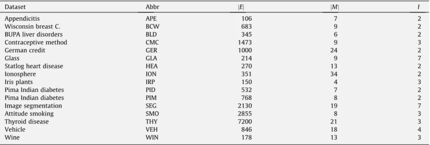
Table 1

Datasets.

Dataset Abbr jEj jMj I

Appendicitis APE 106 7 2

Wisconsin breast C. BCW 683 9 2

BUPA liver disorders BLD 345 6 2

Contraceptive method CMC 1473 9 3

German credit GER 1000 24 2

Glass GLA 214 9 7

Statlog heart disease HEA 270 13 2

Ionosphere ION 351 34 2

Iris plants IRP 150 4 3

Pima Indian diabetes PID 532 7 2

Pima Indian diabetes PIM 768 8 2

Image segmentation SEG 2130 19 7

Attitude smoking SMO 2855 8 3

Thyroid disease THY 7200 21 3

Vehicle VEH 846 18 4

(13)

5.1. Datasets and parameters for the FRF ensemble

To obtain these results we have used several datasets from the UCI repository[2], whose characteristics are shown in Ta-ble 1. It shows the number of examplesðjEjÞ, the number of attributesðjMjÞand the number of classes (I) for each dataset. ‘‘Abbr” indicates the abbreviation of the dataset used in the experiments.

Finally, we use the FRF ensemble with sizeT2 ð100;150Þtrees except for the experiment of Section5.4.1, which will be shown inTable 7. The number of attributes chosen at random at a given node is log2ðj j þ1Þ, wherej jis the number of

available attributes at that node, and each tree of the FRF ensemble is constructed to the maximum size (node pure or set of available attributes is empty) and without pruning.

5.2. Validating the experimental results by non-parametric tests

After the experimental results have been shown, we make an analysis of them in each subsection using statistical tech-niques. Following the methodology of[16]we use non-parametric tests.

We use the Wilcoxon signed-rank test to compare two methods. This test is a non-parametric statistical procedure for performing pairwise comparison between two methods. This is analogous with the pairedt-test in non-parametric statistical procedures; therefore, it is a pairwise test that aims to detect signiﬁcant differences between two sample means, that is, the behaviour of two methods.

When we compare multiple methods, we use the Friedman test and the Benjamin–Hochberger procedure[4]as post-hoc test (this last procedure is more powerful than Bonferroni–Dunn test, Holm test and Hochberger procedure). The Friedman test is a non-parametric test equivalent to the repeated-measures ANOVA. Under the null-hypothesis, it states that the meth-ods are equivalent, so a rejection of this hypothesis implies the existence of differences in the performance of all the methmeth-ods studied. After this, the Benjamin–Hochberger procedure is used as a post-hoc test to ﬁnd whether the control or proposed methods show statistical differences with regard to the other methods in the comparison.

5.3. Behaviour and stability of the FRF ensemble with imperfect data and noise 5.3.1. Management of imperfect data

To introduce ana% of imperfect values in a dataset ofjEjexamples, each of which hasjMjattributes (excluding the class attribute), we select randomlya% jEj jMjvalues of the dataset uniformly distributed among all the attributes. For each va-lue, corresponding to an example and to an attribute, we modify the value. Imperfect data were introduced to both the train-ing and testtrain-ing datasets.

We divided this test in three experiments:

In the ﬁrst experiment, we run the FRF ensemble on datasets in which we have inserted missing values, in both numerical and nominal attributes.

In the second experiment, we run the FRF ensemble on datasets in which we have inserted fuzzy values in the numerical attributes. These fuzzy values correspond to the different fuzzy sets of the fuzzy partition for each numeric attribute of the dataset.

In the third experiment, we inserted tanto missing values como fuzzy values on datasets.

When the value of a numerical attribute of an example from the dataset is chosen to be replaced by a fuzzy value, it is done as follows: since the numerical attribute is partitioned in a fuzzy partition, the value of the attribute will belong, with associated degrees of membership, to one or two fuzzy sets of the partition. We substitute the value of the attribute of that example for the fuzzy set with which the greatest degree of membership was obtained. The percentages of imperfect data

Table 2

Testing accuracies of the FRF ensemble for different percentages of missing values. Dataset Introducing missing values

Without 5% 15% 30%

% Decrease average accuracy

APE 91.13(9.70) MIWF1/MIWLF1 0.82MIWF1/MIWLF1 1.03MWLT2/MWLF2 0.21MIWF1/MIWLF1

BCW 97.31(1.76) MWLT1/MWLT2 0.12MWL2/MWLT2 0.79MWLT2 2.92MWLT2

GER 76.68(3.97) MWLF2 0.70MWLT2 3.86MWLFUS2 5.16MWLFUS2

GLA 77.66(7.36) MWLT2 6.62MWLFUS2 10.95MWL2 17.20MWLT2

ION 96.41(2.89) MIWLF1 0.94MIWF1/MIWLF1 2.66MWLFUS2 6.09MIWF1/MIWLF1

IRP 97.33(3.93) ** 1.23SM1/SM2//MWF1/MWF2 4.11MWF1 16.71MWL2

PIM 77.14(4.88) MWF1 0.82MWF1 2.57MWF1 7.47MWLF2

(14)

inserted in the datasets were 5%, 15%, and 30% in each of the three experiments1_{. In the third experiment, the percentage was} divided into equal parts of missing values and fuzzy values.

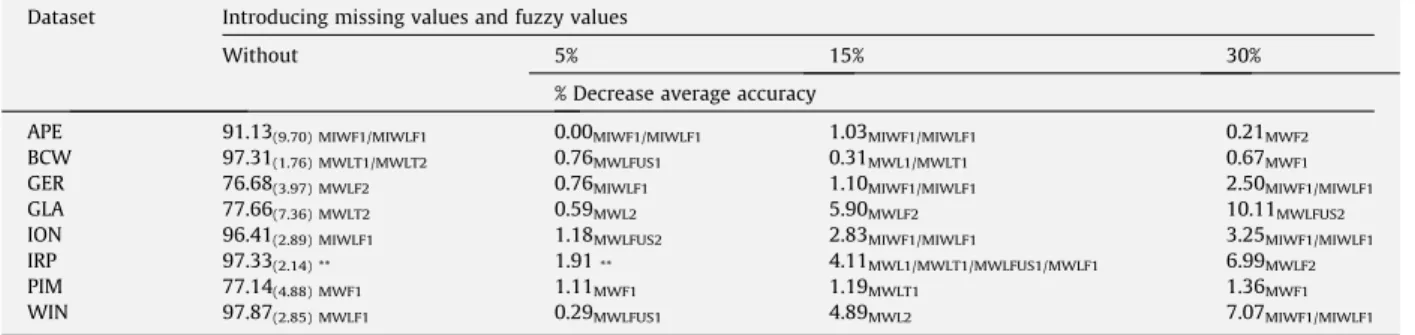
In these experiments, a 10-fold cross validation is independently performed five times using different partitions of the dataset (510-fold cross validation) and we show the percentage of classification average accuracy of the FRF ensemble (mean and standard deviation) in dataset without imperfect data and decrease in the percentage of classification average accuracy of the FRF ensemble in the dataset with imperfect data, together with the combination methods of the FRF ensem-ble which obtains these values (the symbol ‘‘**” indicates that there are more than four methods that obtain that average value). The decrease in the percentage of classification average accuracy, which is shown inTables 2–4, is computed as,

%decrease accuracy¼100ðCPðoriginal_CP_ðÞ_originalCPðimperfect_Þ ÞÞwhereCP(imperfect)is the classiﬁcation average accuracy for the dataset with imperfect data, andCP(original)is the one for the original data.

InTables 2–4it can be observed that the FRF ensemble presents a very stable behaviour in the presence of a signiﬁcant amount of imperfect data.

5.3.2. Effect of noise

In this test, we analyze the effect that noise can cause in the FRF ensemble. We divided this test in two experiments. In the ﬁrst, we ran the FRF ensemble on datasets in which we introduced outlier examples. In the second experiment, we ran the FRF ensemble on datasets in which we inserted data with noise in the class attribute.

5.3.2.1. Introducing outliers in datasets.One way to identify outliers is with the quartile method. This method uses the lower quartile or 25th percentileðQ1Þand the upper quartile or 75th percentileðQ3Þof each attribute of the dataset (theQ2quartile

Table 3

Testing accuracies of the FRF ensemble for different percentages of fuzzy values. Dataset Introducing fuzzy values

Without 5% 15% 30%

APE 91.13(9.70) MIWF1/MIWLF1 0.21MIWF1/MIWLF1 0.82MIWF1/MIWLF1MWLF1/MWLF2 0.21MIWF1/MIWLF1

BCW 97.31(1.76) MWLT1/MWLT2 0.42MWLT1/MWLT2MWLFUS1/MWLFUS2 0.28MWLT1/MWLT2 0.12MWLT1/MWLT2

GER 76.68(3.97) MWLF2 0.08MIWF1/MIWLF1 0.29MIWLF1 0.26MWLF2

GLA 77.66(7.36) MWLT2 1.08MWLF2 0.00SM2 1.31MWF2

ION 96.41(2.89) MIWLF1 0.53MIWLF1 0.46MWLF2 0.94MIWF1/MIWLF1

IRP 97.33(2.14) ** 0.00** 0.00** 0.00**

PIM 77.14(4.88) MWF1 0.52MWF1 0.17MWF1 1.49SM1

WIN 97.87(2.85) MWLF1 0.29MWL2/MWLT2/MWLFUS2/MWLF2 0.51MWLF1/MWLF2 0.75MWF2

Table 4

Testing accuracies of the FRF ensemble for different percentages of missing and fuzzy values. Dataset Introducing missing values and fuzzy values

Without 5% 15% 30%

APE 91.13(9.70) MIWF1/MIWLF1 0.00MIWF1/MIWLF1 1.03MIWF1/MIWLF1 0.21MWF2

BCW 97.31(1.76) MWLT1/MWLT2 0.76MWLFUS1 0.31MWL1/MWLT1 0.67MWF1

GER 76.68(3.97) MWLF2 0.76MIWLF1 1.10MIWF1/MIWLF1 2.50MIWF1/MIWLF1

GLA 77.66(7.36) MWLT2 0.59MWL2 5.90MWLF2 10.11MWLFUS2

ION 96.41(2.89) MIWLF1 1.18MWLFUS2 2.83MIWF1/MIWLF1 3.25MIWF1/MIWLF1

IRP 97.33(2.14) ** 1.91** 4.11MWL1/MWLT1/MWLFUS1/MWLF1 6.99MWLF2

PIM 77.14(4.88) MWF1 1.11MWF1 1.19MWLT1 1.36MWF1

WIN 97.87(2.85) MWLF1 0.29MWLFUS1 4.89MWL2 7.07MIWF1/MIWLF1

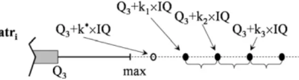
Fig. 3.Distribution of attributeAtriand value ofk.

1

(15)

corresponds to the median andminandmaxcorrespond to the lowest and highest value of each attribute, respectively). We will use this quartile method to generate and insert examples with outlier values in the different datasets.

We will take an outlier value as that which is greater thanQ3þkIQwherekis a given positive constant andIQis the

inter-quartile range. Thus, the datasets with outliers were obtained in the following way: 1. We selected a numerical attributeðAtriÞfor each dataset.

2. For each dataset and its selected attribute Atri, we calculate k¼minfk=Q3þ ðk0:5Þ IQ6ðmax valueAtriinEÞ 6Q₃_þkIQ_g with E being the set of examples from the datasets, k takes values in _f0_:5_;1_;1_:5_;2_;2_:5_;_{. . .}_g and

IQ¼Q3Q1(inter-quartile range),Q1lower quartile (25th percentile),Q3upper quartile (75th percentile), respectively,

of the attributeAtri(seeFig. 3).

3. For each dataset, we select a 1% of examples. 4. We deﬁnek1¼kþ0:5; k2¼kþ1 andk3¼kþ1:5.

5. For each example selected, we modiﬁed the value of the numerical attributeAtriby replacing it by a value chosen

ran-domly from interval½Q3þkiIQ;Q3þ ðkiþ0:5Þ IQfori¼1;2;3. As can be observed (seeFig. 4), we obtain three

possi-ble values for each replacement, depending on k1;k2 and k3. Hence, we will obtain three datasets with outliers

corresponding tok1;k2andk3for each original dataset. This was done only for the training dataset.

We carried out three experiments, one for each dataset obtained in the previous process with the selectedk1;k2andk3.

The experiments were done with a 45-fold cross validation.Table 5shows the percentage of classiﬁcation average accu-racy values (mean and standard deviation) for datasets without outliers and the percentage increase in the classiﬁcation

Fig. 4.Three possible values for generating outliers.

Table 5

Effect for different types of outliers on the FRF ensemble. Dataset Outliers

Without Obtained withk1 Obtained withk2 Obtained withk3

% Increase average error

BCW 97.30(1.48) MWLFUS1/MWLFUS2 1.11MWF1/MWLF1 5.19MWLFUS1/MWLFUS2 3.70MWLFUS1/MWLFUS2

BLD 72.97(5.19) MWF2 3.22MWF2 2.70MWF2 1.59MWF2 CMC 53.62(2.00) MWLF1 0.19MWLT1 0.30MWLT1 0.11MWLF1 GLA 78.38(6.11) MWLT2 1.57MWLT2 3.75MWLT2 1.06MWLT2 HEA 82.87(5.29) MWLT1 4.32MWLT1 1.11MWLF2 4.32MWLT1 ION 94.66(2.19) SM1 6.93MWF1 6.74SM1 5.43SM1 IRP 97.33(2.14) ** 0.00** 0.00** 0.00** PID 79.61(3.27) MWF2 1.62MWF2 0.49MIWLF1 2.11MWF2 PIM 76.53(3.86) MWF1 3.07MWF1 1.79SM1 0.13SM1 SEG 97.19(0.48) MWF1 2.85MWF1 3.91MWF1 3.20MIWLF1

SMO 69.54(1.97) MIWF1/MIWLF1 0.03MIWF1/MIWLF1 0.03MIWF1/MIWLF1 0.03MIWF1/MIWLF1

VEH 75.18(1.91) MWLF2 0.60MWF1 1.93MWF2 1.33MWF2

WIN 97.48(3.23) MWLF1 17.06MWLF1 11.51MWLF1 11.51MWLF1

Table 6

Comparison of tree-based ensembles and classiﬁers with noise data.

Dataset % Increase error Best classiﬁcation method % Increase error Best combination method Hamza et al.[18] Hamza et al.[18] (FRF) (FRF)

BCW 54.84 ST-NLC-G 4.54 MWLFUS2 BLD 16.98 BA-NLC-G 6.78 MWLFUS2 CMC 6.23 ST-NLC-G 0.57 MWLFUS2 HEA 2.08 RF 2.44 MIWF1 PID 5.74 RF 4.42 MWLFUS2 SEG 115.56 RF 81.36 MWF2

SMO 3.07 BA-NLC-G 0.02 MWLT2,MWLFUS2

THY 23.08 RF 18.19 MWF2

(16)

average error between the original data and data with outliers. In addition, the combination method that obtains these val-ues is indicated (the symbol ‘‘**” indicates that there are more than four combination methods that obtain that value). The increase in the percentage of classiﬁcation average error, shown in the Table 5, is computed as %increase error¼ 100ðCEðwith outliers_CE_ð_originalÞCE_ÞðoriginalÞÞwhereCE(with_outliers)is the classiﬁcation average error for the dataset with outliers, and CE(ori-ginal)is the one for the original data.

When we perform the Friedman non-parametric statistical test to compare the average accuracy of these four samples we find no significant differences between them with a 95% confidence level. From these results, we can conclude that introduc-ing outliers further away from the sample causes the FRF ensemble to behave just as if it had no outliers.

5.3.2.2. Introducing noise data in the class attribute.We compared the FRF ensemble with the best technique reported in[18] for the same experiment. The best technique is deﬁned as the one with the lowest percentage increase in the classiﬁcation average error between the original dataset and dataset with noise, with a 10-fold cross validation.

The datasets with noise were obtained in the following way: with probability 10%, we modified the value of the class attribute by replacing it with a value chosen uniformly at random from its other possible values. This was only for the train-ing dataset. Again, noise was introduced into the traintrain-ing datasets via the NIP 1.5 tool[12]. The increase in the percentage of classification average error, which is shown in theTable 6, is computed as %increase error¼100ðCEðnoise_CE_ðÞ_originalCEðoriginal_Þ ÞÞwhere CE(noise) is the classification error for the dataset with noise, andCE(original) is that for the original data.

The results can be seen inTable 6. Again, using the Wilcoxon test to compare the results of[18]and the FRF ensemble, we obtain signiﬁcant differences at 97.3%. With these results, the FRF ensemble has a good behaviour when we introduce noise in the class attribute with an increase of error smaller than in[18].

5.4. Comparing the FRF ensemble with other classiﬁers and ensembles

5.4.1. Comparative of the FRF ensemble and other ensembles using the same base classiﬁer

This subsection summarizes a series of experiments performed to observe the effectiveness of the FRF ensemble when compared with the base classifier and several ensembles built with this base classifier: (1) the base classifier, (2) a boosting based ensemble, (3) a bagging based ensemble, and (4) the FRF ensemble. We also compare the results of the FRF ensemble with the obtained with Breiman’s Random Forest (RF)[17]. We should note that, excluding RF, all ensembles have been built using a fuzzy decision tree as base classifier. The execution of each experiment was done with the same parameters. In this experiment we have made a 45-fold cross validation.Table 7shows the results obtained, indicating the percentage of clas-sification average accuracy (mean and standard deviation).

The results obtained in this experiment clearly show that, for these datasets, the ensembles are always better than the individual classifier. It is also shown that the FRF ensemble is the ensemble that consistently generates the best results. In most cases bagging is better than boosting. When we perform the statistic test on these results, we first apply the Fried-man test, obtaining a rejection of the null-hypothesis with a 99.9% confidence level. That is, it accepts that there are signif-icant differences. When we perform the post-hoc test, we obtain that the FRF ensemble has significant differences with methods RF, fuzzy decision tree (FT), boosting and bagging with a confidence level of 95.98%, where the FRF ensemble is the best method. For other methods we obtain the following: with a 99.9% confidence level it is concluded that RF, FT and boosting are significantly different, where RF is the best of them; and with a 99.7% confidence level it is concluded that bagging, FT and boosting are significantly different.

5.4.2. Comparative with other methods of the literature

In this subsection, we compare and baseline the operation of the FRF ensemble with other classiﬁers and ensembles found in the literature. In each case we will say how the comparison has been made.

Table 7

Testing average accuracies of the FRF ensemble with other ensembles with same base classiﬁer.

Dataset Size RF RF fuzzy tree (FT) Size ensembles Boosting with FT Bagging with FT FRF ensemble BCW 125 97.07(1.89) 95.50(1.75) 125 94.51(1.51) 95.68(1.60) 97.30(1.48) BLD 200 72.68(6.32) 65.14(5.75) 200 65.79(6.23) 71.88(5.89) 72.97(5.19) CMC 120 51.41(2.61) 47.17(2.62) 120 49.08(2.99) 51.49(2.04) 53.62(2.00) GLA 120 78.85(6.05) 72.43(8.34) 50 74.89(6.29) 76.74(5.72) 78.38(6.11) HEA 120 81.48(4.13) 74.26(6.58) 120 77.13(4.63) 81.02(5.13) 82.87(5.29) ION 175 93.45(2.25) 92.59(3.29) 175 94.09(3.59) 93.25(3.12) 94.66(2.19) IRP 120 95.33(1.74) 97.00(2.08) 120 96.67(2.53) 96.67(2.53) 97.33(2.14) PID 125 76.41(2.12) 71.85(3.95) 50 70.54(3.69) 78.05(3.19) 79.61(3.27) PIM 150 75.26(3.51) 67.55(4.53) 150 66.18(3.64) 73.63(2.96) 76.53(3.86) SEG 140 97.85(0.59) 95.54(1.06) 140 96.54(0.77) 97.19(0.66) 97.19(0.48) SMO 100 61.63(0.82) 55.29(2.42) 75 56.36(1.48) 69.50(1.91) 69.54(1.97) THY 150 99.67(0.10) 96.13(0.53) 150 96.26(0.62) 98.25(0.38) 99.17(0.22) VEH 200 76.27(2.73) 67.96(3.94) 200 70.06(3.64) 74.41(3.04) 75.18(1.91) WIN 150 98.03(1.93) 97.19(2.85) 150 97.20(3.45) 97.06(3.36) 97.48(3.23)

(17)

5.4.2.1. Comparative study with other classifiers. We have compared the results of the FRF ensemble with other classifiers, taking the results reported in[20]which compare the classifiers GRA-based (grey relational analysis) and CIGRA-Based (Cho-quet integral-based GRA) with other well known classification methods, including the MLP (multi-layer perceptron), the C4.5 decision tree, radial basis function (RBF), the naive Bayes, the Cart decision tree, the hybrid fuzzy genetic-based machine learning algorithm (GBML) and a fuzzy decision tree.

To examine the generalization ability of the FRF ensemble, we have made a 1010-fold cross validation. Again, we show the percentage of classiﬁcation average accuracy for all methods and in addition the standard deviation for the FRF ensemble together with the combination methods of the FRF ensemble which obtain these values. The results can be seen in the Table 8.

When we make the statistical analysis for these results, we first apply the Friedman’s test getting a rejection of the null-hypothesis with a 99.6% confidence level. That is, we accept that there are significant differences. When we make the post-hoc analysis, we obtain that the FRF ensemble has significant differences with the methods GRA, CIGRA, MLP, C4.5, RBF, Bayes, Cart and Fuzzy D. Tree with a 98.2% confidence level and with GBLM with a 96.9% confidence level, and the FRF ensemble is the best method. We conclude that the FRF ensemble is an effective classifier and that it exhibits very good performance.

5.4.2.2. Comparative study with other ensembles. In Ref.[18]we ﬁnd a comparative study of the best tree-based ensembles. We will compare the results of the FRF ensemble with those reported in that work. A 10-fold cross validation is made. Then, we very brieﬂy describe the tree-based ensembles used in that work with which we make the comparison. The ensembles used are:

1. Single Tree with pruning (CART). 2. Bagging with 100 trees (CART).

3. RF: Random Forest with 100 trees (number of attributes chosen at random at a given node islog2ðjMj þ1ÞwhereMis the

set of attributes).

4. BO: Boosting (arcing) with 100 and 250 trees (CART). Split Criteria – G: Gini, E: Entropy, T: Twoing, WLC: With Linear Combination, NLC: No Linear Combination.

The results can be seen inTable 9. On comparing the FRF ensemble with the best proposed ensemble in[18], with a 95.2% conﬁdence level, there are signiﬁcant differences between the two methods, with the FRF ensemble being the best.

Table 8

Comparative accuracies of the FRF ensemble and other classiﬁers. Dataset Technique

FRF GRA CIGRA MLP C4.5 RBF Bayes Cart GBLM Fuzzy D.Tree

APE 91.04(10.12) MIWF1/MIWLF1 86.00 88.70 85.80 84.90 80.20 83.00 84.90 – – BCW 97.14(1.78) MWLT1/MWLT2 96.20 96.80 96.50 94.70 96.60 96.40 94.40 96.70 96.80 GER 76.41(3.96) MWLF2 73.00 74.20 71.60 73.50 75.70 70.40 73.90 – – GLA 76.82(7.85) MWLT2 57.40 63.20 68.70 65.80 46.70 71.80 63.60 65.40 66.00 ION 96.13(2.99) MIWLF1 88.50 92.60 92.00 90.90 94.60 85.50 89.50 – 86.50 IRP 97.33(4.58) ** 95.70 96.10 96.00 94.00 98.00 94.70 92.00 94.70 96.10 PIM 76.70(4.34) MWF1 74.90 76.20 75.80 72.70 75.70 72.20 74.70 75.80 73.10 WIN 97.64(3.19) MWLF1 93.30 96.20 98.30 93.30 94.90 94.40 87.60 95.10 91.20 Table 9

Comparison with tree-based ensembles. Dataset

BCW BLD CMC HEA PID SEG SMO THY VEH

Best classiﬁcation error [18]

2.64 25.80 47.39 17.78 22.93 1.60 34.05 0.28 23.40 Best classiﬁcation

error method[18]

RF RF RF RF RF RF BO(100)WLC-E BO(100)WLC-E BO(250)WLC-G Best classiﬁcation

error – FRF

2.49 24.67 46.57 14.44 19.35 2.55 30.47 0.78 23.17 Best classiﬁcation error

combination method

MWLT1/MWLT2/ MWLFUS1/ MWLFUS2

MWLFUS1 MWLF1 MIWF1 MWLFUS2 MWF2 MWLT2 MWLFUS2

MIWF1/ MIWLF1

(18)

6. Summary

In this paper, we present an ensemble based on fuzzy decision trees called FRF ensemble. We realize a hybridization of the techniques of random forest and fuzzy trees for training. The proposed ensemble has the advantages of imperfect data man-agement, of being robust to noise and of having a good degree of classiﬁcation with relatively small sizes of ensembles.

We have defined various methods to combine the outputs of base classifiers of the FRF ensemble. These methods are based on the combination methods used frequently in the literature to obtain the final decision in ensembles. Hence we have defined:

Non-trainable methods: Within this group there are methods based on simple majority vote.

Trainable explicitly dependent methods: In this group are the methods that use weights deﬁned by the degree of satisfaction of the example to classify the different leaves reached and weights learned for the trees of the FRF ensemble.

Trainable implicity dependent methods: In this group there are methods that use weights learned for the trees of the FRF ensemble.

We have presented experimental results obtained by applying the FRF ensemble to various datasets. Overall, the combi-nation methods that achieve better performances are the weighted combicombi-nation methods, compared to non-weighted meth-ods typically used in random forest based ensembles. Among the weighted methmeth-ods those using a weighting based on membership function have better performance, obtaining the best results in 65% of total tests performed. Although most of the methods of combination have the same computational cost, we highlight the increased cost of local fusion based methods. Nevertheless, these last methods have a good performance in the datasets with noise in the class attribute.

In particular, on the imperfect datasets (with missing and fuzzy values) the results obtained by the FRF ensemble are very promising. The FRF ensemble has a good performance with datasets with fuzzy values. The weighted combination methods perform better than non-weighted methods when working with these datasets.

With datasets with outliers the FRF ensemble shows a good performance and we can conclude that introducing outliers further away from the sample causes the FRF ensemble to behave just as if it had no outliers. When making the comparison with datasets with noise in the class attribute, the FRF ensemble shows a clear advantage over other proposals and the MWL-FUS2 combination method shows the best behaviour in most cases. So, the FRF ensemble is robust to noise.

When we compare the FRF ensemble with the base classifier, RF and ensembles using the same base classifier, the FRF ensemble obtains the best results. On comparing the results of the FRF ensemble with those obtained by a series of classifiers and multi-classifiers we conclude that the FRF ensemble is an effective classifier and that it obtains the best results in most cases.

Moreover, all these conclusions have been validated by applying statistical techniques to analyze the behaviour of differ-ent methods or algorithms compared in each experimdiffer-ent.

Acknowledgements

Supported by the project TIN2008-06872-C04-03 of the MICINN of Spain and European Fund for Regional Development. Thanks also to the Funding Program for Research Groups of Excellence with code 04552/GERM/06 granted by the ‘‘Fundación Séneca”, Murcia, Spain.

References

[1] H. Ahn, H. Moon, J. Fazzari, N. Lim, J. Chen, R. Kodell, Classiﬁcation by ensembles from random partitions of high dimensional data, Computational Statistics and Data Analysis 51 (2007) 6166–6179.

[2] A. Asuncion, D.J. Newman, UCI Machine Learning Repository, University of California, School of Information and Computer Science, Irvine, CA, <http:// www.ics.uci.edu/mlearn/MLRepository.html>.

[3] R.E. Banﬁeld, L.O. Hall, K.W. Bowyer, W.P. Kegelmeyer, A comparison of decision tree ensemble creation techniques, IEEE Transactions on Pattern Analysis and Machine Intelligence 29 (1) (2007) 173–180.

[4] Y. Benjamini, Y. Hochberg, Controlling the false discovery rate: a practical and powerful approach to multiple testing, Journal of the Royal Statistical Society Series B 57 (1995) 289–300.

[5] P. Bonissone, F. Xue, R. Subbu, Fast meta-models for local fusion of multiple predictive models, Applied Soft Computing Journal (2008), doi:10.1016/ j.asoc.2008.03.06.

[6] P.P. Bonissone, J.M. Cadenas, M.C. Garrido, R.A. Díaz-Valladares, A fuzzy random forest: fundamental for design and construction, in: Information Processing and Management of Uncertainty in Knowledge-Based Systems International Conference (IPMU2008), Málaga, Spain, 2008, pp. 1231–1238. [7] L. Breiman, Bagging predictors, Machine Learning 24 (2) (1996) 123–140.

[8] L. Breiman, Random forests, Machine Learning 45 (1) (2001) 5–32.

[9] J. Casillas, L. Sánchez, Knowledge extraction from data fuzzy for estimating consumer behavior models, in: Proceeding Fuzzy IEEE, Vancouver, BC, Canada, 2006.

[10] J.M. Cadenas, M.C. Garrido, R.A. Díaz-Valladares, Hacia el Diseño y Construcción de un fuzzy random forest, in: Proceedings in II Simposio sobre Lógica Fuzzy y Soft Computing, Zaragoza, Spain, pp. 41–48.

[11] J.M. Cadenas, M.C. Garrido, R. Martínez, Una estrategia de particionamiento fuzzy basada en combinación de algoritmos, in: Proceedings in XIII Conferencia de la Asociación Española para la Inteligencia Artiﬁcial, Sevilla, Spain, 2009, pp. 379–388.

[12] J.M. Cadenas, J.V. Carrillo, M.C. Garrido, R. Martínez, E. Muñoz, NIP 1.5 – A tool to handle imperfect information on datasets, Murcia University, <http:// heurimind.inf.um.es/NIP/index.htm>, 2008.

(19)

[13] T.G. Dietterich, An experimental comparison of three methods for constructing ensembles of decision trees: bagging, boosting, and randomization, Machine Learning 40 (2) (2000) 139–157.

[14] A. Fernández, M.J. del Jesus, F. Herrera, Hierarchical fuzzy rule based classiﬁcation systems with genetic rule selection for imbalanced data-sets, International Journal of Approximate Reasoning 50 (3) (2009) 561–577.

[15] Y. Freud, R.E. Schapire, A decision-theoretic generalization of on-line learning and an application to boosting, Journal of Computer and System Sciences 55 (1) (1997) 119–139.

[16] S. García, A. Fernández, J. Luengo, F. Herrera, A study statistical techniques and performance measures for genetics-based machine learning: accuracy and interpretability, Soft Computing,doi:10.1007/s00500-0080392-y.

[17] M. Hall, E. Frank, G. Holmes, B. Pfahringer, P. Reutemann, I.H. Witten, The WEKA data mining software: an update, SIGKDD Explorations 11 (1) (2009) 10–18.

[18] M. Hamza, D. Larocque, An empirical comparison of ensemble methods based on classiﬁcation trees, Statistical Computation and Simulation 75 (8) (2005) 629–643.

[19] T.K. Ho, The random subspace method for constructing decision forests, IEEE Transactions on Pattern Analysis and Machine Intelligence 20 (8) (1998) 832–844.

[20] Y-C. Hu, A novel fuzzy classiﬁer with Choquet integral-based grey relational analysis for pattern classiﬁcation problems, Soft Computing 12 (2008) 523–533.

[21] J. Jang, Structure determination in fuzzy modeling: a fuzzy CART approach, in: Proceedings IEEE Conference on Fuzzy Systems, Orlando, USA, 1994, pp. 480–485.

[22] C.Z. Janikow, Fuzzy decision trees: issues and methods, IEEE Transaction on Systems, Man and Cybernetics, Part B 28 (1) (1998) 1–15.

[23] L. Koen-Myung, L. Kyung-Mi, L. Jee-Hyong, L. Hyung, A fuzzy decision tree induction method for fuzzy data, in: Proceedings IEEE Conference on Fuzzy Systems, Seoul, Korea, 1999, pp. 22–25.

[24] L.I. Kuncheva, Fuzzy vs Non-fuzzy in combining classiﬁers designed by boosting, IEEE Transaction on Fuzzy Systems 11 (6) (2003) 729–741. [25] L.I. Kuncheva, Combining Pattern Classiﬁers: Methods and Algorithms, John Wiley & Sons, Inc., 2004.

[26] L.F. Mendonça, S.M. Vieira, J.M.C. Sousa, Decision tree search methods in fuzzy modeling and classiﬁcation, International Journal of Approximate Reasoning 44 (2) (2007) 106–123.

[27] D. Opitz, R. Maclin, Popular Ensemble Methods: an empirical study, Journal of Artiﬁcial Intelligence 11 (1999) 169–198.

[28] A. Otero, J. Otero, L. Sánchez, J.R. Villar, Longest path estimation from inherently fuzzy data acquired with GPS using genetic algorithms, in: Proceedings on EFS, Lancaster, UK, 2006.

[29] P. Pulkkinen, H. Koivisto, Fuzzy classiﬁer identiﬁcation using decision tree and multiobjective evolutionary algorithms, International Journal of Approximate Reasoning 48 (2) (2008) 526–543.

[30] L. Sánchez, M.R. Suárez, J.R. Villar, I. Couso, Mutual information-based feature selection and partition design in fuzzy rule-based classiﬁers from vague data, International Journal of Approximate Reasoning 49 (3) (2008) 607–622.

[31] L. Sánchez, I. Couso, J. Casillas, Genetic learning of fuzzy rules based on low quality data, Fuzzy Sets and Systems 160 (2009) 2524–2552. [32] R.E. Schapire, Theoretical views of boosting, in: Proceedings of 4th Eur. Conf. Computational Learning Theory, 1999, pp. 1–10.