Model predictive control based on LPV models with parameter-varying delays

(1)

Model predictive control based on LPV models with parameter-varying

delays

Fatemeh Karimi Pour, Vicenc¸ Puig and Carlos Ocampo-Martinez

Abstract— This paper presents a Model Predictive Control (MPC) strategy based on Linear Parameter Varying (LPV) models with varying delays affecting states and inputs. The pro-posed control approach allows the controller to accommodate the scheduling parameters and delay change. By computing the prediction of the state variables and delay along a prediction time horizon, the system model can be modified according to the evaluation of the estimated state and delay at each time instant. Moreover, the solution of the optimization problem associated with the MPC design is achieved by solving a series of Quadratic Programming (QP) problem at each time instant. This iterative approach reduces the computational burden compared to the solution of a non-linear optimization problem. A pasteurization plant system is used as a case study to demonstrate the effectiveness of the proposed approach.

I. INTRODUCTION

In modern times of industrialization, research on advanced control algorithms for complex dynamic systems is still very active. Controlling these complex systems is one of the most important challenges in control engineering. On the other hand, time delays may arise in the dynamics of real systems, such as communication systems, chemical processes, and transportation systems [1]. The effect of time delay in a process increases the control problem. The delays can affect the states, inputs or/and outputs, and they can be time-varying or constant, unknown or known, deterministic or stochastic depending on the considered system. One of the main, successful and popular advanced control strategies for industrial processes is Model Predictive Control (MPC) [2]. MPC based on linear models is typically used in pro-cess control where the on-line optimization problem can be formulated as a convex optimization problem by either linear programming or Quadratic Programming (QP). This assumption is suitably considered for typical processes. However, most of the real systems show nonlinear behav-iors. In order to reduce the conservativeness, the idea of controlling nonlinear systems considering linear parameter varying (LPV) models has been widely investigated in the literature [3]. The main advantage of LPV models is that the system nonlinearities are embedded into the varying parameters, which make the nonlinear system become a linear-like system with varying parameters [4].

*This work has been partially funded by the Spanish State Research Agency (AEI) and the European Regional Development Fund (ERFD) through the projects DEOCS (ref. MINECO DPI2016-76493) and SCAV (ref. MINECO DPI2017-88403-R).

All authors are with Advanced Control Systems Group, Universi-tat Politècnica de Catalunya, Institut de Robòtica i Informàtica Indus-trial (CSIC-UPC), C/. Llorens i Artigas 4-6, 08028 Barcelona, Spain {fkarimi, vpuig, cocampo}@iri.upc.edu

Recently, many researchers focuses on the robust model predictive control (RMPC) based on the linear model with constant or varying delays [5], [6]. In [7], a RMPC with constant state delay by using linear matrix inequalities (LMIs) term is proposed. The work of [8] proposes an MPC algorithm for uncertain time varying systems with state delays. Besides, a synthesis strategy for predictive control based on LPV models with state delays was provided in [8]. The results were further extended for the system with input delayed in [9]. However, there exist only a few MPC methods that consider time-delayed LPV model [10], [11]. In [10], authors proposed a parameter-dependent state-feedback controller based on LPV model with parameter-varying time delay and proved the stability by using parameter-dependent Lyapunov functionals. However, there exists a limitation to apply input constraints which are required when controlling many practical plants. Also, an RMPC based on LPV model with state delay was presented in [11] by using a Lyapunov function augmented with the current state and the time-delayed states. But, still delay is considered to be constant in the RMPC.

The main contribution of this paper consists in designing an improved LPV-based MPC strategy in order to formu-late an optimization problem that exploits the functional dependency of scheduling variables and varying delays to develop a prediction strategy with the numerically suitable solution. This solution is iteratively forced to an accurate solution, thereby avoiding the use of non-linear optimization. In addition, the optimization problem is decomposed into a series of QP problems that are solved at each time instant. Finally, the small-scale pasteurization plant that presents nonlinear behavior with varying delays is used in order to test the effectiveness of the proposed approach.

The paper is structured as follows. In Section II, the formulation of MPC based on an LPV model with varying delays is introduced. Then, the LPV-based MPC approach for LPV model with varying delay is presented in Section III. In Section IV, results of applying the proposed control strategy to the pasteurization system are presented. Finally, in Section V, the conclusion of this work are drawn.

II. PROBLEMSTATEMENT

Consider the following discrete-time state-space LPV model with parameter-varying delays in inputs and states:

x(k+ 1) =A(θ(k))x(k) +Aτ(θ(k))x(k−τ(θ(k)))

+B(θ(k))u(k) +Bτ(θ(k))u(k−τ(θ(k))), y(k) =C(θ(k))x(k) +Cτ(θ(k))x(k−τ(θ(k))),

(2)

where x ∈ R , u ∈ R and y ∈ R are the

state vector, input vector and output vector, respectively. Moreover, A(θ(k)) ∈ Rnx×nx_, _B₍_θ₍_k₎₎ _∈

Rnx×nu _and

C(θ(k))∈Rny×nx _{are system matrices with the appropriate}

dimensions, which depend affinely on the varying parameter

θ(k)∈Θ∀k≥0whereΘis a given compact set. Moreover,

τ is a scalar function representing the parameter-varying delay and satisfies 0 ≤ τm ≤ τ(θ(k)) ≤ τM, where τM

and τm are the upper bound and lower bound of τ(θ(k)).

Throughout this paper, it is assumed that (A(θ), B(θ)) is stabilizable for allθ∈Θ.

The MPC controller design with a quadratic objective function subject to input and states constraints based on the LPV model (1) can be formulated as follows:

[u(i|k), u(i + 1|k), ..., u(Np −1|k)]>, where u˜(k) is the

decision sequence of Np predicted control inputs whereNp

is number of predication horizon. Moreover, w1 ∈Rnx×nx

and w2 ∈ Rnu×nu _{are positive definite weighting matrices}

that establish the trade-off between state and the control input effort, respectively. The super-index pis the squared norm that is used for this paper. Furthermore, the setsXandUare

defined as

x∈X=M{x(k)∈Rnx|x≤x(k)≤x}, ∀k, (3a) u∈_U=M{u(k)∈_Rnu_|_u_≤_u₍_k₎_≤_u_}_, _∀_k, _(3b)

where vectors x ∈ _Rnx _and _x ∈

Rnx _{determine the}

minimum and maximum possible state values of the system, respectively. Similarly, u ∈ _Rnu _and _u _∈

Rnu determine

the minimum and maximum possible value of manipulated variables, respectively. The control law is applied in a receding horizon manner, that is, at time k the optimal sequence of control input is defined and then, only the first optimal control input is applied to the system. Then, the new measurements are applied to update the initial conditions and then the optimization problem is solved again using the receding horizon rule. Also, x(i|k)is the predicted state at timei, withi= 1, ..., Np, obtained by starting from the state x(0|k) =x(k).

The LPV model can not be evaluated before solving the optimization problem (2) because the future state sequence is not known. Indeed x(i|k)depends not only on the future control inputsu(k), but also on the future scheduling param-eters θ(k) and delay, where for a general LPV system are

not assumed to be known a priori but only to be measurable online at current timek. In addition, in the case of a system with varying delay, the delay varies with the scheduling variables. Hence, predicting the future states regarding the dynamic of the system is more difficult. But, for a quasi-LPV system, where the scheduling parameters θ(k) are defined by x(k) and u(k), the delay and state trajectory can be predicted.

III. PROPOSEDAPPROACH

This section proposes an MPC controller design in order to solve the optimization problem of an LPV model with parameter-varying delay where the parameters and delays change along the prediction horizon. The idea is to find a solution to the problem (2) by solving an online optimization problem as a QP problem. The solution for this problem is based on the estimation the scheduling variables and subsequently delay into the prediction horizon and using them to update the system matrices of the model that used by the MPC controller. In fact, the sequence of the control input is used to modify the delay and system matrices of the model used along the prediction horizon. Therefore, the sequence of states and predicted parameters can be obtained from the control sequenceu˜(k)as

φ([x>(k) x˜>(k)]>,u˜(k)), respectively. The vector Θ(k) includes parameters from time k to k+Np−1 whilst the

state prediction is accomplished for timek+ 1 tok+Np.

Consequently, by using the vectors (4) and (5), thex˜(k) can be simply formulated as follow

˜

x(k) =A(Θ(k))x(k) +Aτ(Θ(k))x(k−τ˜(Θ(k)))

+B(Θ(k))˜u(k) +Bτ(Θ(k))˜u(k−τ˜(Θ(k))),

(6)

whereA andAτ ∈Rnx×nx _and _B _and_B

τ ∈Rnx×nu _are

given by (7) and (8). By using (6) and augmented block diagonal weighting matrices w˜1 = diagNp(w1) and w˜2 =

diagNp(w2), the cost function (2a) can be represented in

(3)

A(Θ(k)) =        I A(ˆθ(k)) A(ˆθ(k+ 1))A(ˆθ(k)) .. . A(ˆθ(k+Np−1))A(ˆθ(k+Np−2)). . . A(ˆθ(k))        , (7) and B(Θ(k)) =        0 0 0 . . . 0 B(ˆθ(k)) 0 0 . . . 0 A(ˆθ(k+ 1))B(ˆθ(k)) B(ˆθ(k+ 1)) 0 . . . 0 .. . ... . .. . .. ... A(ˆθk+Np−1). . . A(ˆθ(k+ 1))B(ˆθ(k)) A(ˆθk+Np−1). . . A(ˆθ(k+ 2))B(ˆθ(k+ 1)) . . . B(ˆθk+Np−1)) 0        . (8)

for all i∈_Z[0,Np−1]. Since the predicted states x˜(k) in (6)

are linear in control inputs u˜(k), the optimization problem can be solved as a QP problem, which is significantly easier than solving a nonlinear optimization problem.

However, the variation of delay at each iteration and inside the prediction horizon makes difficulty to solve the optimiza-tion problem considering a specific value of the predicoptimiza-tion horizon length because for solving the optimization problem as MPC design based on a model with delay, the length of prediction horizon should include delay. Hence, during solv-ing the MPC optimization problem the prediction horizon length should be adapted considering the delay value. Thus, because of the change of the prediction horizon, the size of states and inputs vectors should be adapted accordingly. In order to summarize the proposed method, Algorithm 1 is introduced.

IV. CASESTUDYAPPLICATION

A. Case study description

In order to show the effectiveness of the proposed ap-proach in the real case study, the pasteurization process that is described in [12] is chosen as a real case study. The pasteurization model is represented in terms of behavioral equations of each subsystem, consisting of holding tube, power, water pump, heat exchanger and hot water tank. The non-liner model of the pasteurization system is considered as

˙

x=f(x, x(t−τ), u, u(t−τ), ω(t)), (10) where, x= [T1T2T2rT4Tin]>∈R5, u= [N1N2 P]>∈

R3 and ω = [Ta] ∈ R1 are states, inputs and disturbance

of the pasteurization system, respectively. In addition, state equation f : _X×_U −→ _X and _X ⊆ _R5 _{is presented in}

Appendix. The physical properties, process data and param-eters related of the pasteurization model in the identification process are described in Table II and III in Appendix.

The identification procedure to estimate some unknown parameters of the nonlinear model is based on [13]. The idea of the method is to compare, the data obtained from the real set-up with the data obtained by simulating part of the continuous time non-linear model of the pasteurization

process. This is formulated as an optimization problem that allows finding the parameter values that better approximate the real system in the least squares sense. Due to the lake of space, this can be only illustrated briefly by estimating unknown parameters of the hot-water tank temperature. The identification procedure is based on the knowledge of the non-linear model of the hot-water tank temperature (13b). It is assumed to have at accessNT2 sets of dataP

j₍_k₎_{, N}j

1(k)

for the hot-water tank temperature where j = 1, ..., NT2

and k = 1, ..., Kj where Kj is the number of samples of

the j−th set of data. The identification process determines the minimum of the following objective function over the unknown parametersα1, α2andα3:

JT2 = NT₂ X j=1 Kj X k=1 T₂j(k)−Tˆ₂j(k) 2 , (11)

where Tˆ₂j(k) is the simulation provided by (13b). In the same manner, the identification procedure is applied based on the other equation of the nonlinear model for estimating the remaining unknown parameters. By using the non-linear embedding approach [14], the state-space LPV model of the pasteurization plant can be expressed as follows:

A=        a11 0 0 0 0 0 a22 a23 0 0 0 a32 a33 a34 a35 0 a42 a43 a44 a45 0 0 a53 0 a55        , B=        b11 0 0 0 b22 b23 b31 b32 0 b41 b42 0 b51 0 0        Aτ=        0 aτ,12 aτ,13 aτ,14 aτ,15 0 0 0 0 0 0 0 0 0 0 0 0 0 0 0 0 0 0 0 0        , Bd=        bd,11 bd,21 bd,31 bd,41 0        , Bτ =        bτ,11 bτ,12 0 0 0 0 0 0 0 0 0 0 0 0 0        , C= ₁ ₀ ₀ ₀ ₀ 0 1 0 0 0 , (12)

where the value of matrix parameters are introduced in Appendix. The most important objective of the pasteurization procedure is to ensure that the pasteurization temperature is attained and preserved as close the set-point amount for a

(4)

delay

1: k←−0

2: repeat

3: i←−0

4: if k= 0 then

5: Solve the optimization problem (9) by considering

θ(0|k) 'θ(1|k) 'θ(2|k) '... 'θ(Np−1|k)

6: Calculate Θ(k)and˜τ(k)using ˜x(k)andu˜(k)

7: else 8: Determine Θ(k) = {θˆ(i|k)}Np−1 i=0 and τ˜(k) = {τ(i|k)}Np−1 i=0 , where θˆ(i|k) = ψ(x(i|k − 1 + 1), u(i|k−1))andτ(i|k) =φ(x(i|k−1+1), u(i|k−1)

9: Compute the difference value g= ˜τ(k)−τ˜(k−1)

10: if g≤0 then 11: x˜(k) = {x(i|k)}Np−|g| i=0 and u˜(k) = {u(i|k)}Np−1−|g| i=0 12: else 13: xg˜ (k) = (˜x(Np−1),[1, g]) ˜ x(k) ={˜x(k),xg˜ (k)} 14: end if

15: Solve the optimization problem (9)

16: i←−i+ 1

17: end if

18: Apply the first value of the optimal input sequence to the system

19: Define Θ0(k+ 1) =ψ(˜x1(k),u˜0(k))and ˜τ0(k+ 1) =

φ(˜x1(k),u˜0(k))

20: Modify the size of Np,Np> τ

21: k←−k+ 1

22: until end

pre-established time. According to this, theT1temperature is

the output of the holding tube for monitoring the temperature of the product after the pasteurization procedure, controlling

T1 to track set-points is one of the main objectives. On the

other hand, the hot-water tank is the thermal energy source used to heat the product and proper system operation, T2

should always be greater than T1 due to achieve the final

temperature desired. Hence, in order to guarantee the energy for the process,T2 should be controlled.

B. Results and Discussion

In this section, the proposed algorithm based on the system with constant delay and varying delay is compared by the state-of-the-art NMPC approach based on the system with the same information. The comparison is made both in terms of closed-loop performance and computational timing performance. All simulation and computations have been carried out using a commercial computer with i7 2.40-GHz Intel core processor with 12 GB of RAM running MATLAB R2016b. The optimization problems (9) and (2) are solved by using the linear and nonlinear programming solvers available in YALMIP (Lofberg, 2004). The solution of (11) is found by means offminconMATLAB function of the Optimization

Toolbox. All tests are applied by same prediction horizon, parameters and constraints as mentioned in Table I.

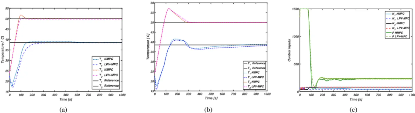
In order to validate the values obtained by identification, the simulation of the non-linear model has been compared by the data obtained from the real system. Figures 1a) and 1b) present the comparison of the tracking response results that obtained under the LPV-based MPC approach and the NMPC controller based on the pasteurization model with the constant and varying delay during the prediction horizon, respectively. Moreover, the responses of the control actions using a controller based on proposed approach and NMPC controller that considered the model with the constant and varying delay in the prediction horizon are provided in Figures 1c) and 2, respectively. The comparison of compu-tational timing performance of LPV-based MPC and NMPC is summarized in Table III. Actually, in the pasteurization process, the delay of the system is depended on the control action. Therefore, in the constant delay case, the delay of the system is varied at each time instant k, but during the prediction horizon are considered as constant delays, where the value of delay in the next iteration k+ 1 is computed by the first elements of the optimal input. For more clarity of how the delay is varied in the new proposed approach during prediction horizon, Figure 3 shows the evolution of delay when it is considered constant and varying during the prediction horizon.

According to these results, it can be observed that the proposed LPV-based MPC controller is tracked and reached the set-point and the performance of the proposed algorithm is almost the same as the NMPC one. In terms of the computational timing performance, there is a quite clear difference: although the average time proposes that the LPV-based MPC is on average four times faster than the NMPC, in fact, the algorithms are only as good as its worst-case performance, in which case it is clear that the proposed approach is approximately an order of magnitude faster. To sum up, the simulation results show that the proposed LPV-based MPC controller is able to control LPV time-delay systems while improving the performance of the closed-loop system and achieving the specified set-point.

V. CONCLUSIONS

This paper focused on the design of a model predictive control algorithm based on a class of Linear Parameter Varying (LPV) models with parameter varying delay. The constrained optimization problem for an LPV model with parameter varying and constant delay is solved iteratively by a series of QP problems while the scheduling parameters and delay are calculated at each time instant. The model with varying delay is predicted in the horizon by using the previous sequence of scheduling variable and state of the model. Based on the variation of the delay, the prediction horizon length is changed during the simulation. The pro-posed approach is considered a fast computation time and appreciably faster than other mentioned approach. For future research, It would be interesting to implement the proposed approach on the real benchmark of the pasteurization plant

(5)

0 100 200 300 400 500 600 700 800 900 1000 Time [s] 15 20 25 30 35 40 45 50 55 Temperature [ C] T1 NMPC T 1 LPV-MPC T2 NMPC T2 LPV-MPC T1 Reference T 2 Reference (a) 0 100 200 300 400 500 600 700 800 900 1000 Time [s] 15 20 25 30 35 40 45 50 55 60 Temperature [ C] T 1 Reference T 2 Reference T 1 NMPC T 1 LPV-MPC T 2 NMPC T 2 LPV-MPC (b) 0 100 200 300 400 500 600 700 800 900 1000 Time [s] 0 500 1000 1500 Control inputs N 1 NMPC N 1 LPV-MPC N 2 NMPC N 2 LPV-MPC P NMPC P LPV-MPC (c)

Fig. 1: Different assessments. (a) output temperatures (Delay is constant during the prediction horizon). (b) control inputs (Delay is varied during the prediction horizon). (c) control inputs (Delay is constant during the prediction horizon).

TABLE I: Comparison of each strategies timing performance

Configuration Maximum time Average time Standard deviation r.m.s. error (T1) r.m.s. error (T2)

NMPC constant delay intoNP 4.4540 2.0091 0.9071 4.9703 4.3479

LPV-MPC constant delay intoNP 0.1640 0.0785 0.0078 5.243 4.425

NMPC varying delay intoNP 24.887 6.9558 3.9441 5.117 4.7791

LPV-MPC varying delay intoNP 0.8771 0.2480 0.1409 5.402 4.820

0 100 200 300 400 500 600 700 800 900 1000 Time [s] 0 500 1000 1500 Control inputs N₁ NMPC N₁ LPV-MPC N₂ NMPC N₁ LPV-MPC P NMPC N₁ LPV-MPC

Fig. 2: Evaluation of the control inputs (Delay is varied during the prediction horizon)

1 2 3 4 5 6 7 8 9 10 11

Number of prediction horizon

8.5 9 9.5 10 10.5 Delay

Constant delay during N_p

Varying delay during N_p

Fig. 3: Comparison of delay during the prediction horizon

by considering the uncertainty and sensitivity of disturbance in the model.

APPENDIX

For obtaining the pasteurization model, physical principle based fundamental laws such as energy balances and heat exchanger design are utilized to describe the main processes of the plant. Therefore, Energy balance and Bernoulli’s law produces the following set of dynamical equations:

dT1 dt = 2 M1CP (−U AT1(t) +T4(t−τ) 2 −Ta) −F1Cp(T1(t)−T4(t−τ))− dT4(t−τ) dt (13a) dT2 dt =α1P(t)−F2Cp(T2(t)−T2r(t))−α2T2(t) +α3 (13b) dT2r dt =F1(T4(t)−Tin(t)) +α4F2(T2(t)−T2r(t)) −α5(T2(t)−Ta)−α6−α7N1(t) (T4(t)−Tin(t)) +α8N2(t)(T2(t)−T2r(t)) −α9(T4(t)−Tin(t)) +α10(T2(t)−T2r(t)) (13c) dT4 dt =−F1(T4(t)−T in(t)) +α11F2(T2(t)−T2r(t)) −α12−α13N1(t)(T4(t)−T in(t)) +α14N2(t)(T2(t)−T2r(t)) (13d) dTin dt = α15(N1(t)−α16)(T1(t)−Tin(t)) M2 , (13e)

(6)

whereF1=α17(N1(t)−α16),F2=α18(N2(t)−α19), and

the delay of system is

τ(t) =−α20−α21(N1(t))3+α22(N1(t))2 −α23N1(t) +α24.

The value of entries for the state-space matrices for the controller used in (12) are presented as follows:

a11= −U A M1Cp −F1Cp a22=−F2Cp−α2 a23=F2Cp a32=F2α4+N2(k)α8+α10−α5 a33=−F2α4−N2(k)α8−α10 a34=−N1(k)α7+F1−α9 a35=N1(k)α7−F1+α9 a42=F2α11+N2(k)α14 a43=−F2α11−N2(k)α14 a44=−N1(k)α13−F1 a45=N1(k)α13+F1 a53= α15(N1(k)−α16) M2 a55= −α15(N1(k)−α16) M2 b11=−α17Cp(T1(k)−T4(k−τ)) b22=−α18Cp(T2(k)−T2r(k)) b23=α1 b31= (α17−α7)(T4(k)−Tin(k)) b32= (α18α14+α8)(T2(k)−T2r(k)) b41= (−α17−α7)(T4(k)−Tin(k)) b42= (α18α11+α14)(T2(k)−T2r(k)) b51= α15(T2r(k)−Tin(k)) M2 bd,11=α25Ta bd,21=α3 bd,31=α5Ta−α6 bd,41=α12 aτ,12=−F2α11−N2(k)α14 aτ,13=F2α11+N2(k)α14 aτ,14= U A M1Cp +F1Cp+F1+α13N1(k) aτ,15=α13N1(k)−F1 bτ,11= (α17+α13)(T4(k−τ)−Tin(k−τ)) bτ,12= (−α11α18−α14)(T2(k−τ)−T2r(k−τ))

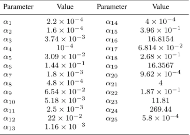
Moreover, Tables II and III collect the information about both the model and simulation parameters, respectively.

TABLE II: Physical properties and process data

Parameter Description Value Unit

U constant of convective heat transfer 10 [Wm2_/K]

A area of the tank 0.0248 [m2_]

Cp specific heat of the hot-water 4.186 [J/g◦C]

M1 mass of liquid inside the tank 82 [g]

M2 mass product inside the regeneration section 24.85 [g]

Ta room temperature 24.5 [◦C]

T1 temperature at the end of holding tube [0,80] [◦C]

T2 temperature inside hot water tank [0,80] [◦C]

T2r returned water temperature from the heat exchanger [0,80] [◦C]

T4 temperature at the exit of heat exchanger [0,80] [◦C]

Tin temperature after regeneration section [0,80] [◦C]

N1 percentage speed of feeding pump [40-80] [%]

N2 percentage speed of hot-water pump [20-80] [%]

P power of the electric resistor [0-1500] [W]

Parameter Value Parameter Value

α1 2.2×10−4 α14 4×10−4 α2 1.6×10−4 α15 3.96×10−1 α3 3.74×10−3 α16 16.8154 α4 10−4 α17 6.814×10−2 α5 3.09×10−2 α18 2.68×10−1 α6 1.44×10−1 α19 16.3567 α7 1.8×10−3 α20 9.62×10−4 α8 4.8×10−4 α21 4 α9 6.54×10−2 α22 1.87×10−1 α10 5.18×10−3 α23 11.81 α11 2.5×10−3 α24 269.44 α12 22×10−2 α25 5.8×10−4 α13 1.16×10−3 REFERENCES

[1] P. Segovia, L. Rajaoarisoa, F. Nejjari, E. Duviella, V. Puig, Input-delay model predictive control of inland waterways considering the backwater effect, in: 2nd IEEE Conference on Control Technology and Applications, 2018, to appear.

[2] F. Karimi Pour, V. Puig, C. Ocampo-Martinez, Comparative assess-ment of lpv-based predictive control strategies for a pasteurization plant, in: Control, Decision and Information Technologies (CoDIT), 2017 4th International Conference on, IEEE, 2017, pp. 0821–0826. [3] F. Karimi Pour, V. Puig, C. Ocampo-Martinez, Multi-layer

health-aware economic predictive control of a pasteurization pilot plant, International Journal of Applied Mathematics and Computer Science 28 (1) (2018) 97–110.

[4] F. Karimi Pour, V. Puig, G. Cembrano, Health-aware lpv-mpc based on a reliability-based remaining useful life assessment, IFAC-PapersOnLine 51 (24) (2018) 1285–1291.

[5] Y. Ge, J. Wang, C. Li, Robust stability conditions for dmc controller with uncertain time delay, International Journal of Control, Automa-tion and Systems 12 (2) (2014) 241–250.

[6] S. Lee, S. Jeong, D. Ji, S. Won, Robust model predictive control for lpv systems with delayed state using relaxation matrices, in: American Control Conference (ACC), 2011, IEEE, 2011, pp. 716–721. [7] B. Capron, M. Uchiyama, D. Odloak, Linear matrix inequality-based

robust model predictive control for time-delayed systems, IET control theory & applications 6 (1) (2012) 37–50.

[8] S. C. Jeong, P. Park, Constrained mpc algorithm for uncertain time-varying systems with state-delay, IEEE Transactions on Automatic Control 50 (2) (2005) 257–263.

[9] B. Ding, L. Xie, W. Cai, Robust mpc for polytopic uncertain systems with time-varying delays, International Journal of Control 81 (8) (2008) 1239–1252.

[10] F. Wu, K. M. Grigoriadis, Lpv systems with parameter-varying time delays: analysis and control, Automatica 37 (2) (2001) 221–229. [11] L. Zhang, W. Xie, Z. Zhong, J. Wang, Robust model predictive control

synthesis for state-delayed systems with randomly occurring input saturation nonlinearities, Transactions of the Institute of Measurement and Control 40 (1) (2018) 179–190.

[12] F. Karimi Pour, C. Ocampo-Martinez, V. Puig, Output-feedback model predictive control of a pasteurization pilot plant based on an lpv model, in: Journal of Physics: Conference Series, Vol. 783, IOP Publishing, 2017, p. 012029.

[13] F. Nejjari, D. Rotondo, V. Puig, M. Innocenti, Quasi-lpv modelling and non-linear identification of a twin rotor system, in: Control & Automation (MED), 2012 20th Mediterranean Conference on, IEEE, 2012, pp. 229–234.

[14] A. Kwiatkowski, M.-T. Boll, H. Werner, Automated generation and assessment of affine lpv models, in: Decision and Control, 2006 45th IEEE Conference on, IEEE, 2006, pp. 6690–6695.