Muhammad Saif-ur-Rehman1,8 , Robin Lienkämper1, Yaroslav Parpaley2, Jörg Wellmer3, Charles Liu4, Brian Lee4, Spencer Kellis5, Richard Andersen5, Ioannis Iossifidis6, Tobias Glasmachers7 and Christian Klaes1,9
1 Faculty of Medicine, Ruhr-University Bochum, Bochum, Germany
2 Department of Neurosurgery, University Hospital Knappschaftskrankenhaus Bochum, Bochum, Germany
3 Ruhr-Epileptology, Department of Neurology, University Hospital Knappschaftskrankenhaus Bochum, Bochum, Germany
4 USC Neurorestoration Center, Keck School of Medicine of USC, Los Angeles, California, United States of America
5 Department of Biology and Biological Engineering, California Institute of Technology, Pasadena, California, United States of America
6 Department of Computer Science, Ruhr West University of Applied Sciences, Mülheim an der Ruhr, Germany
7 Institute for Neural Computation, Ruhr-University Bochum, Bochum, Germany
8 Faculty of Electrical Engineering and Information Technology, Ruhr-University Bochum, Bochum, Germany
E-mail: [email protected]
Received 10 December 2018, revised 16 April 2019 Accepted for publication 1 May 2019
Published 23 July 2019 Abstract
Objective. In electrophysiology, microelectrodes are the primary source for recording neural data (single unit activity). These microelectrodes can be implanted individually or in the form of arrays containing dozens to hundreds of channels. Recordings of some channels contain neural activity, which are often contaminated with noise. Another fraction of channels does not record any neural data, but only noise. By noise, we mean physiological activities unrelated to spiking, including technical artifacts and neural activities of neurons that are too far away from the electrode to be usefully processed. For further analysis, an automatic identification and continuous tracking of channels containing neural data is of great significance for many applications, e.g. automated selection of neural channels during online and offline spike sorting. Automated spike detection and sorting is also critical for online decoding in brain–computer interface (BCI) applications, in which only simple threshold crossing events are often considered for feature extraction. To our knowledge, there is no method that can universally and automatically identify channels containing neural data. In this study, we aim to identify and track channels containing neural data from implanted electrodes, automatically and more importantly universally. By universally, we mean across different recording technologies, different subjects and different brain areas. Approach. We propose a novel algorithm based on a new way of feature vector extraction and a deep learning method,
Journal of Neural Engineering
SpikeDeeptector: a deep-learning based
method for detection of neural spiking
activity
M Saif-ur-Rehman et al Printed in the UK 056003 JNEIEZ © 2019 IOP Publishing Ltd 16 J. Neural Eng. JNE 1741-2552 10.1088/1741-2552/ab1e63Paper
5Journal of Neural Engineering IOP
Original content from this work may be used under the terms of the Creative Commons Attribution 3.0 licence. Any further distribution of this work must maintain attribution to the author(s) and the title of the work, journal citation and DOI.
2019
9 Author to whom any correspondence should be sent.
https://doi.org/10.1088/1741-2552/ab1e63 J. Neural Eng. 16 (2019) 056003 (20pp)
which we call SpikeDeeptector. SpikeDeeptector considers a batch of waveforms to construct a single feature vector and enables contextual learning. The feature vectors are then fed to a deep learning method, which learns contextualized, temporal and spatial patterns, and classifies them as channels containing neural spike data or only noise. Main results. We trained the model of SpikeDeeptector on data recorded from a single tetraplegic patient with two Utah arrays implanted in different areas of the brain. The trained model was then evaluated on data collected from six epileptic patients implanted with depth electrodes, unseen data from the tetraplegic patient and data from another tetraplegic patient implanted with two Utah arrays. The cumulative evaluation accuracy was 97.20% on 1.56 million hand labeled test inputs. Significance. The results demonstrate that SpikeDeeptector generalizes not only to the new data, but also to different brain areas, subjects, and electrode types not used for training. Clinical trial registration number. The clinical trial registration number for patients implanted with the Utah array is NCT 01849822. For the epilepsy patients, approval from the local ethics committee at the Ruhr-University Bochum, Germany, was obtained prior to implantation. Keywords: deep learning, convolutional neural networks, contextual learning,
brain–computer interface, spike sorting
S Supplementary material for this article is available online (Some figures may appear in colour only in the online journal)
Introduction
The human brain contains approximately 100 billion neurons (Herculano-Houzel 2009). Neurons communicate by propa-gating action potentials (Hodgkin and Huxley 1952), also referred to as ‘spikes’. The spikes generated by individual neurons (sometimes called ‘units’) can be recorded with the help of microelectrodes (Kita and Wightman 2008). State-of-the-art development in microelectronics has allowed the fab-rication of tiny but dense microelectrode arrays, containing hundreds of channels (Frey et al 2008, Lambacher et al 2011, Berényi et al 2013, Spira and Hai 2013). As a result, the activ-ities of several hundreds or even thousands of neurons (Harris et al 2017) can be recorded simultaneously. Spikes recorded from only one neuron are called single-unit activity (SUA). However, often it is not possible to determine if spikes origi-nate from only a single source or multiple neurons in which case the activity is called multi-unit activity (MUA).
Spike sorting is used to separate the activity of each neuron and is usually done manually or semi-automatically (Abeles and Goldstein 1977, Gibson et al 2012, Matthews and Clements 2014). However, there are also some studies in which automatic spike sorting methods are proposed (Spacek et al 2009, Takekawa et al 2012, Bongard et al 2014, Carlson et al 2014, Pachitariu et al 2016, Yger et al 2018). A standard spike sorting pipeline includes spike event detection and assignment to specific neurons (SUA). Most current spike sorting methods require human input of some form and are therefore prone to subjectivity and bias. Using a fully auto-mated process could reduce the subjective bias and drastically reduce the time needed for spike sorting.
Most existing spike sorting algorithms use band-pass filtering, spatial whitening and threshold crossing before qualifying an incoming waveform as an event. Finally, they apply clustering on qualified events. This generally involves at least one or more
manual processing steps (Lewicki 1998, Einevoll et al 2012, Marre et al 2012). Moreover, previous studies have shown that a considerable fraction of dense implanted microelectrode arrays does not record any neural data, but only external artifacts with high amplitudes and/or noise (Lewicki 1998, Hill et al 2011, Klaes et al 2015, Rey et al 2015). Human involvement in spike sorting can be reduced by automatically identifying and dis-carding meaningless channels at the first stage before any further analysis. However, the background noise is composed of several complex signals, including neuronal activity too far away from the electrode to be useful, external artifacts and noise generated by surrounding electrical components (Lewicki 1998, Einevoll et al 2012). There are studies in which noise modeling is studied (Yang et al 2011), for example in Yang et al (2011). In that study, the authors enhanced the signal-to-noise ratio by estimating neu-ronal signatures, noise shaping, and adaptive bandpass filtering. However, the proposed model requires some training data to optimize the value of the parameters in each recording session for each electrode separately. Therefore, nonstationary behavior of noise is a problem for automatically discarding meaningless channels (Chung et al 2017).
In recent years it has been demonstrated that powerful models can be learned with the help of huge amounts of labeled data and deep artificial neural network architectures (Krizhevsky et al 2012). A specific architecture, convolutional neural net-works (CNN) (LeCun et al 1998), in combination with huge labeled datasets (Jia et al 2009, Stallkamp et al 2011) has trans-formed the field of computer vision and provided many state-of-the-art results for image classification, object detection and tracking (Guo et al 2017). In the current study, we used the same approach to solve a different problem: discarding chan-nels that do not contain spikes. After collecting and labeling a large amount of spike data, we successfully trained a deep neural network that enables us not only to detect but also to track the channels containing neural data. As a result, noise channels can
M Saif-ur-Rehman et al
be discarded before doing further analysis. Our system acts as a universal spike detector, which can also be used in online analysis. By universal we mean that the trained model can be employed to detect and track the channels containing neural data recorded from different subjects, across different brain areas and even with different types of recording hardware, without any additional prep aration. To support this claim, we evaluated SpikeDeeptector on the data recorded from eight different sub-jects of different age and genders, recorded using different types of microelectrodes across different areas of the brain.
The presented method is based on supervised deep learning, which means ground-truth labels are required to define the cost function (Kotsiantis 2007). It is difficult even for an expert neuroscientist to judge a single event without the con-text of other events. Here, we introduce a new way of labeling that considers a batch of waveforms from the same channel, instead of a single waveform, to construct a feature vector. This approach establishes context for classifier learning and decision making. Our data set contains 1.56 million labeled feature vectors. By mimicking the way humans sort spikes, SpikeDeeptector can generalize across different data sources. We achieve an overall classification accuracy of 97.20%.
SpikeDeeptector can be employed to select meaningful channels during online decoding for brain–computer interfaces (BCIs), where previously unsorted action potentials were used to extract feature vectors (Fraser et al 2009, Schwartz 2004, Koyama et al 2009, Todorova et al 2014, Klaes et al 2015). Such feature vectors also include threshold crossing events of channels which do not contain neural data. In contrast, SpikeDeeptector discards all the channels that do not contain neural data. Thus, it allows to consider only those channels where at least a minimum number of neural spikes is present. Furthermore, SpikeDeeptector can be applied to the last step of spike sorting, which often requires a human to accept or reject clusters found by an algorithm (Hill et al 2011, Kadir et al 2014, Rossant et al 2016). With SpikeDeeptector, it is also possible to automatically detect which clusters are noise and which clusters contain a unit.
Materials and methods
Approvals
For this study we used data from tetraplegic patients implanted with Utah arrays (Blackrock Microsystems, Salt Lake City,
UT) and patients who were implanted with depth electrodes in preparation for epileptic surgery. Tetraplegic patients were recruited for two different BCI studies (Aflalo et al 2015, Klaes et al 2015). These studies were approved by the institu-tional review boards at the California Institute of Technology (Pasadena, CA), Rancho Los Amigos National Rehabilitation Center (Downey, CA), and the University of Southern California (USC) (Los Angeles, CA). Further approval details are available from (Aflalo et al 2015, Klaes et al 2015). For the epilepsy patients, approval from the local ethics committee at the Ruhr-University Bochum, Germany, was obtained prior to implantation. Epilepsy patients were implanted for medical reasons and we obtained informed consent from each patient before they participated in the study.
Implantation information
We collected data from a total of eight patients (seven males, one female), aged 20–63 years. Six of the patients were implanted with microelectrodes in preparation for epilepsy surgery using a Behnke-Fried configuration (Fried et al 1999). The microelectrodes were coupled in a group of 8 or 16 indi-vidual microwires with platinum coated tips. The other two patients were tetraplegics recruited for a BCI study and were implanted with Utah microelectrode arrays (Aflalo et al 2015, Klaes et al 2015). A single Utah array consists of 100 micro-electrodes arranged in a 10 × 10 grid with the four corner electrodes left unconnected during manufacture. The place-ment of the Utah array was based on a functional magnetic resonance imaging (fMRI) task conducted prior to implant-ation; details of the array placement and surgery are described in Aflalo et al (2015) and Klaes et al (2015). The Utah array electrodes were 1.0–1.5 mm long and presumably recorded signals from cortical layer 5 (Aflalo et al 2015, Klaes et al 2015). Electrodes had platinum-coated tips and were spaced 400 µm apart. The location of the microelectrodes or elec-trode arrays is shown in table 1 along with the total number of recording sessions for each patient.
Behavioral setup
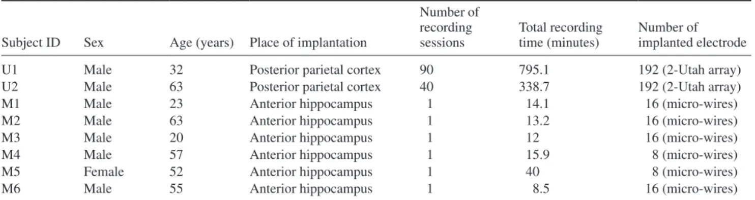
The subjects engaged in various behavioral tasks. More infor-mation about the behavioral tasks of subject U1 and U2 can be found in previous studies (Aflalo et al 2015, Klaes et al 2015). The epilepsy patients performed a reaching task in a Table 1. Demographic information with implantation details.
Subject ID Sex Age (years) Place of implantation
Number of recording
sessions Total recording time (minutes) Number of implanted electrode
U1 Male 32 Posterior parietal cortex 90 795.1 192 (2-Utah array)
U2 Male 63 Posterior parietal cortex 40 338.7 192 (2-Utah array)
M1 Male 23 Anterior hippocampus 1 14.1 16 (micro-wires)
M2 Male 63 Anterior hippocampus 1 13.2 16 (micro-wires)
M3 Male 20 Anterior hippocampus 1 12 16 (micro-wires)
M4 Male 57 Anterior hippocampus 1 15.9 8 (micro-wires)
M5 Female 52 Anterior hippocampus 1 40 8 (micro-wires)
M6 Male 55 Anterior hippocampus 1 8.5 16 (micro-wires)
virtual reality environment, programmed in Unity 3D (Unity Technologies, San Francisco, CA, USA) and using the HTC Vive virtual reality system (HTC Corporation, New Taipei, Taiwan), or remained idle during recording.
Data collection
In the group of tetraplegic subjects, data was collected over a period of two years in two–four study sessions per week. From the group of epilepsy patients, data were gathered over the course of one year with one study session per subject. Data were recorded using a Neural Signal Processor (Blackrock Microsystems, Salt Lake City, UT). Analog electrical activity was amplified and digitized at a sampling rate of 30 kHz. Spike candidates (events) were extracted with a thresholding proce-dure (Lewicki 1998). The threshold for waveform detection was set to −4.5 times the root-mean-square of the high-pass filtered, full-bandwidth signal with cutoff frequency 250 Hz. Similar settings were used in Klaes et al (2015) to select the mean-ingful channels and extract feature vectors (unsorted threshold crossing) for online decoding. However, to evaluate the robust-ness of the spike detection algorithm, different threshold settings were used (see Evaluation of robustness). Each detected wave-form consists of 48 samples and represents a time duration of 1.6 ms, containing the 15 samples before and 32 samples after the threshold crossing event. The value at each sampling interval is the corresponding ampl itude represented in micro-volts.
Data labeling
We cast the problem of spike classification as a super-vised learning task. This means that ground-truth labels were required to train a machine learning model. In a single
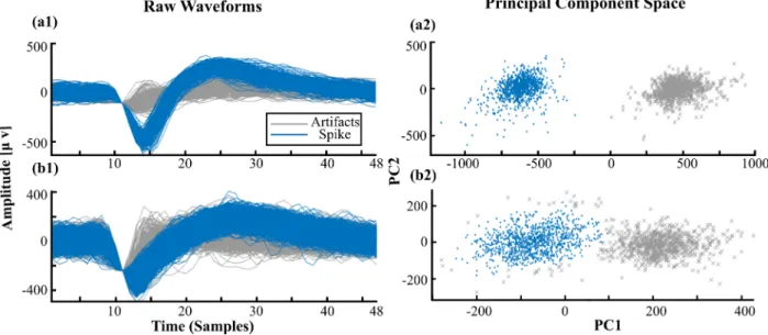
recording session, a single channel records hundred and some-times thousands of unlabeled waveforms. Moreover, we con-sidered eight subjects and 136 recording sessions, resulting in 31.21 million unlabeled waveforms which may correspond to neural events (action potentials) or any other external events (e.g. artifacts from muscle activity or noise). We labeled the data in a semi-automatic method consisting of the following steps: first, we applied principal component analysis (PCA) on all detected waveforms of a channel. Second, we visualized the first two principal components of a subset of waveforms (see figures 1(a2) and (b2)), which capture the direction of highest variability in the data. After visual inspection, we employed a Gaussian mixture model (GMM) on the datapoints in PCA space to assign them to clusters, as shown in figures 1(a2) and (b2). The number of clusters with their corre sponding centroids (initial points) were defined manually. In some cases, semi-automatic labeling provides unsatisfactory results. Therefore, in such cases after visual inspection of the clustered points, the waveforms were entirely manually labeled.
Batch size
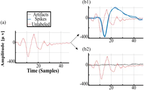
It is hard even for expert neuroscientists to classify a single event as a spike (neural activity) or as an artifact (non-neural activity) in the absence of other events (figure 2(a)). However, when a batch of waveforms of the same channel is considered, the decision becomes much easier if the waveform in ques-tion is a spike (figure 2(b2)) or an artifact (figure 2(b1)). Here, we tried to replicate the way humans sort spikes by including context in our feature vectors. A single feature vector is con-structed by concatenating a batch of waveforms, regardless of their category, thus, enabling SpikeDeeptector to aggregate the statistics of the inputs in a better way.
Figure 1. The process of labeling data for two different kinds of channels. (a1) Labeled waveforms of a channel. (a2) First two principal components of the waveforms in (a1), colored to reflect the result of the clustering algorithm (GMM). The two clusters are easily discriminable: the blue cluster corresponds to neural data and the grey cluster corresponds to artifact. (b1) Labeled waveforms of another channel recorded during the same recording session as (a1). (b2) First two principal components of the waveforms in (b1). Cluster centroids (initial points) were defined manually and allowed the GMM to approximate the probability distribution functions (PDFs). Here, two clusters are not well separated and visual inspection is required. As a result of visual inspection, a few waveforms along the boundaries of clusters were re-labeled manually. After visual inspection and re-labeling, blue cluster corresponds to neural data and grey cluster corresponds to artifacts.
M Saif-ur-Rehman et al
Concretely, a single feature vector x is constructed by con-catenating a batch of b waveforms of length w (in samples) together, resulting in a vector xRb×w. The batch size b is always
a positive integer (bN+) and is considered a hyperparameter. We labeled a feature vector x as a ‘spike’ (i.e. containing a spike) if at least one of the concatenated events was labeled as a spike during the labeling. Alternatively, if all the concat-enated events represent non-neural activities, then x was labeled as an artifact. For example, for b=20, x would com-prise twenty successive events of a channel concatenated together, and if any of the twenty events was labeled as a spike then, the x was labeled as a spike. Alternatively, if all of twenty individual waveforms were labeled as artifacts, then the x was labeled as an artifact.
Here, we only try to classify which batch of the waveforms contain spikes, and not how many and which of the wave-forms in batch represents spikes. Individual event classifica-tion would be the next step.
Data distribution for training algorithm and evaluation of generalization
The complete dataset contains 31.21 million labeled wave-forms. Using a batch size of b=20, that yields 1.56 million labeled feature vectors. The total number of feature vectors resulting from every single individual during recording ses-sions are shown in table 2.
In machine learning, generalization is the most significant quality of the algorithm. That means the evaluation perfor-mance of the algorithm on unseen data plays a pivotal role. Therefore, for training the algorithm, we used a small subset of data, compiled from the first six recording sessions of a subject U1. This training dataset comprised 40 657 feature vectors (2.6% of the total dataset). We then evaluated the trained model on the portion of data not used for training.
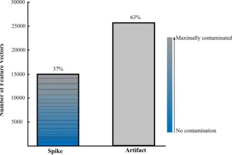
Figure 3 illustrates the distribution of the labeled feature vectors of both classes within the training set. The ‘spike’ class contains feature vectors with varying numbers of events repre-senting artifacts, starting from no-contamination (0 artifacts) to maximally-contaminated (19 artifacts), whereas the feature vectors representing the ‘artifact’ class contain events that exclusively represent artifact/noise. In the available dataset, the spike class provided only 37% of feature vectors (15 024), while the artifact class holds the remaining 63% of the feature vectors (25 633). To avoid biases while training the algorithm, we also prepared a more balanced dataset by performing sub-sampling on the data of both classes. We selected a dataset
D={x1,y1,. . . .,xN,yN} with N=30 000 labeled
examples, where xi refers to i
th feature vector and yi to the
corresponding class label. From each class, 15 000 feature vectors were selected at random.
We then sliced the dataset D into a training set Dtr
con-taining 70% percent of the data and a validation set Dva
con-sisting of the remaining 30%. Dtr was used to optimize the
parameters of the machine learning model and the hyper-parameters of the employed optimization algorithm during training. Dva was used to evaluate how well the machine
learning model performs on unseen data during training. Figure 2. Illustrative example: explains the process of construction of the feature vectors by concatenating the batch of waveforms
and shows the significance of Contextual learning. (a) Shows the single unlabeled waveform, (b1) and (b2): shows the concatenated w waveforms of two different channels representing neural data (spikes) and external artifacts. (b1): shows the unlabeled waveform, when put into context of other events can be assigned as artifact. (b2): shows the similar unlabeled waveform, when put into context of other events can assigned with label of spike.
Table 2. Number of feature vectors per patient. Patient id No. of feature vectors
U1 756 802 U2 436 898 M1 3980 M2 5251 M3 874 M4 13 589 M5 342 951 M6 591 J. Neural Eng. 16 (2019) 056003
This validation error was used as a stopping criterion for the training process. Training terminated if the validation error stopped decreasing or remained the same for six consecutive epochs.
SpikeDeeptector algorithm
The machine learning models were trained on Dtr, with
the goal to predict the correct label yi for each feature
vector xi using the output of a learnable parametric decoder
g(xi;θ):xi∈Rb×w→yi by learning the parameters θ,
itera-tively from Dtr.
We implemented SpikeDeeptector in two variations, SpikeDeeptector CNN and SpikeDeeptector FNN, to compare two of the most popular forms of neural network architectures. SpikeDeeptector CNN follows the standard architecture for CNN (LeCun et al 1998) and SpikeDeeptector FNN follows the standard architecture for fully connected neural networks (FNN) (Goodfellow et al 2016). Both variants followed the standard end-to-end machine learning pipeline. End-to-end learning is decomposed in two parts: The first part maps the raw feature space xi into the more meaningful feature space Φ (xi;θΦ) with the learnable parameter matrices θΦ. The
second part consist of a classifier f with the parameter matrix θf, which maps the feature space Φ into decision space g. The
parameters θΦ and θf were learned simultaneously using Dtr
by iteratively minimizing a single cost function.
Input representation and the architecture of SpikeDeeptector convolutional neural network (SpikeDeeptector CNN)
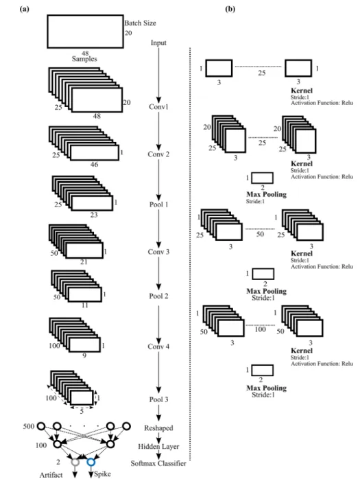
We represented the input as a 2D array with the number of time steps as width and the batch size as height (figure 4).
To classify raw input, we employed the standard architec-ture of CNN used in computer vision tasks, as explained in Krizhevsky et al (2012) and Guo et al (2017). This generic CNN architecture can extract a wide range of features.
SpikeDeeptector CNN contains four convolutional layers and three pooling layers, followed by a fully connected neural network with one hidden layer and a Softmax classifier (Duan et al 2003) as an output layer (see figure 4). During forward propagation, each filter at each layer is convolved across the width and height of the input volume and then slides with stride = 1 over the width and height of the input volume. The result consists of 2D convolved feature maps. These feature maps are then further processed through nonlinear activa-tion maps. We used Rectified Linear Units (ReLUs), where
f(x) =max(x, 0), as the activation function (Nair and Hinton 2010).
The first convolutional layer performs convolution across time and tries to learn temporal patterns from the training data as shown in figure 4. The second convolutional layer performs convolution across space (batch size) and tries to learn the spatial pattern; as a result, it enables contextual learning (see figure 4). The subsequent convolutional layers perform convo-lution across time as shown in figure 4. The size and number of filters at each convolutional layer is illustrated in figure 4.
Except for the 1st convolutional layer, each convolutional layer is followed by a pooling layer. We used max pooling to downsample the convolved feature map and to extract more abstract features. The size of each pooling window has height 1 and width 2 in the architecture of SpikeDeeptector CNN defined in figure 4.
We padded zeros across the width of the input volume. The zero padding was also added across the width before per-forming downsampling at conv3 and conv4 in figure 4. Figure 3. Distribution of training data and construction of the feature vector from the batch of waveforms, subject id: U1, Number of sessions: 6. In this example, with batch size = 20, 20 waveforms were concatenated to get a single feature vector. The range of ‘spike’ class feature vectors starts from no contamination, where every single concatenated waveform represents spike event, and ends at maximally contaminated, where 19 of the concatenated waveforms represent artifact events and only one waveform represents spike event. The feature vectors representing the ‘artifact’ class were created by concatenating the waveforms that exclusively represent artifacts events. 37% of data represents feature vector of the spike class and the remaining 63% of data represents feature vectors of the artifact class.
M Saif-ur-Rehman et al
Regularization techniques and optimization algorithm
We used batch normalization as a regularization technique, which standardizes intermediate outputs of SpikeDeeptector CNN to zero mean and unit variance, for the training exam-ples equal to mini-batch size (Ioffe and Szegedy 2015). This helps the employed optimization algorithm during training by keeping inputs closer to normal distribution. The batch nor-malization is applied to the output of the convolutional layer before nonlinearity (ReLUs), as suggested in the original paper by (Ioffe and Szegedy 2015). We applied dropout as another regularization technique, which randomly sets the values of some input neurons to zero (Srivastava et al 2014). Finally, we
added an L2 regularization (Krogh and Hertz 1991) term in the cross-entropy cost (Mannor et al 2005) function J as shown in equation (1), which ensures small values of all weight param-eters (θw) to prevent the domination of a single weight
param-eter on the decision of the classifier. The equation contains two terms. The first term is the usual cross-entropy cost to penalize misclassifications, if it predicts gi(0, 1) instead of the true
label yi{0, 1} for the ith training example xi. The second
term represents the sum of the square of all the weights in the above defined architecture, also referred to as L2 regulariza-tion. This term is scaled by a factor λ
2n, where λ is a (positive)
hyperparam eter and n is the mini-batch size.
Figure 4. Architecture of SpikeDeeptector CNN. (a) Process of mapping input space into decision space. The input is convolved with layers of kernels to get convolved feature maps. The pooling layer downsamples the convolved feature maps. The output of each layer becomes the input of the subsequent layer. Finally, the Softmax classifier is used to produce an output decision. (b) Size, stride, and number of kernels along with employed activation function to get the convolved feature map. Max pooling is used to downsample the convolved feature map. The size and stride of the pooling is also documented.
J(θ) =−1 n n i=1 [yiln (gi) + (1−yi) ln (1−gi)] + λ 2n θw θw2. (1) We used the mini-batch gradient descent with momentum (Qian 1999) as an optimization technique to update the values of weights and biases. The mini-batch gradient decent with momentum considers n training examples to compute a moving average of the gradients (see equation (2)) and then update the weights and biases in a single iteration (θj
rep-resents jth learnable parameter). The required derivatives were calculated by employing the backpropagation algorithm (Rumelhart et al 1986). The term γ in equation (3) is referred as momentum, which is also a hyperparameter.
Vt=γV(t−1)+ (1 −γ) 1 n n m=1 ∂j(θ) ∂θjm (2) θj:=θj−αVt. (3) Tuning of hyperparameters
The learning rate α in the mini-batch gradient descent with momentum (SGDM, equation (3)) started at α=0.1 and was tuned in a piecewise manner, decreasing by a factor of 10 every 5 training epochs. The momentum γ in SGDM (equa-tion (2)) was selected to be 0.9, so that the algorithm consid-ered the last 10 iterations to calculate the moving average Vt
of the gradients (equation (3)). Besides that, the mini-batch size n in equation (2) depends on the available GPU-memory. We used n=256, which was the optimized value for our
hardware.
We performed a grid search from 0 to 5, with a step size of 0.2, to tune λ of L2 regularization (see equation (1)) and found λ=1.8 to be the optimized value. We also used the
early stopping criteria to avoid overfitting by monitoring the validation error on validation data Dva, at each epoch. If
the validation error of six consecutive epochs increased or remained the same, the training terminated. Lastly, dropout regularization used a probability of 0.5 to determine whether to drop an input neuron.
We have compared the classification accuracy of SpikeDeeptector CNN with another variant of SpikeDeeptector called SpikeDeeptector fully connected neural network.
The architecture of SpikeDeeptector Fully connected neural network (SpikeDeeptector FNN)
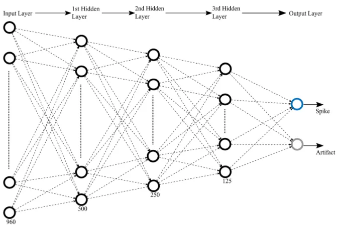
The feature matrix x∈Rb×w was first reshaped into a
vector x∈R(b×w)×1 (see figure 5). Here, the batch size b was considered 20 and w = 48, resulting in a feature vector x∈R960×1. The input feature vector propagates forward from input to hidden layers to output layer (figure 5). The number of neurons in the hidden layers are 500, 250 and 125, and the output layer contains two neurons.
We used Rectified Linear Units (ReLUs), with f(x) =max(x, 0), as an activation function (Nair and Hinton Figure 5. Architecture of SpikeDeeptector fully connected neural network. The input propagates through the input layer, three hidden layers, and an output layer. The number of neurons in each hidden layer are 500, 250, 125; there are two neurons in the output layer. Neurons of the following layer are fully connected to the neurons of the preceding layer.
M Saif-ur-Rehman et al
2010) and Softmax classifier at the last layer (Duan et al 2003).
We used the same regularization and optimization tech-niques as explained in section Regularization techniques and optimization algorithm.
We tuned the hyperparameters of the above defined archi-tecture, in a similar way as described in section Tuning of hyperparameters. However, the optimized value of λ for L2 regularization was found to be 2.4 using the same grid search method described above.
We used the ‘Deep learning’ and the ‘Neural Networks’ tool boxes of MATLAB (The MathWorks, Inc) to define and train the deep-learning algorithms. The source code is avail-able online (https://github.com/saifhanjra/SpikeDeeptector). Assigning labels to channels
The current SpikeDeeptector algorithm can only predict the labels of feature vectors (see section SpikeDeeptector algo-rithm). However, the main aim of this study is to classify the given channel as neural or artifact. Therefore, we introduced a very simple criterion to assign labels to entire channels y(channel)predby calculating the mode of the predicted
out-putsypred of all the feature vectors of the given channel (see
equation (4)).
y(channel)pred=mode(ypred).
(4) We predicted the labels of all channels (see equation (4)) and assigned reliability tags of those predictions which fall in three defined categories: reliable prediction, partially reliable prediction, and unreliable prediction. To assign the reliability tag to the predicted output of the channel y(channel)pred, we calculated percentage of y(channel)pred from predicted out-puts ypred. If the calculated percentage is greater than 80%,
it will be considered as a reliable prediction; if it is between 80% and 60%, it will be considered as partially-reliable; and,
if it is between 50% and 59%, then it will be considered as an unreliable prediction. The thresholds (percentages) of the defined reliability state show the certainty of acquired deci-sions and can be freely adjusted.
Results
Training and evaluation
We compiled a training dataset from the first six recording sessions of subject U1. The distribution of training data and the exact number of feature vectors cast from each patient is explained in section Data distribution for training algorithm and evaluation of generalization. We trained SpikeDeeptector CNN and SpikeDeeptector FNN on the Dtr
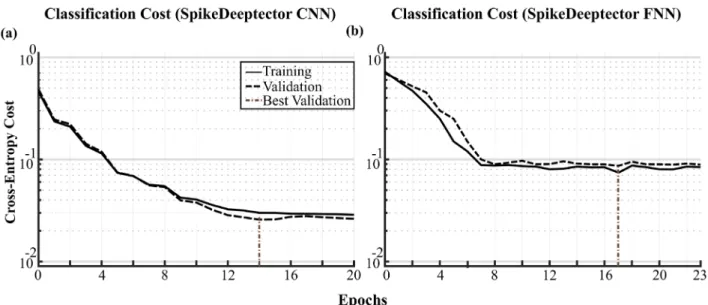
(training data). The training and the validation loss (regular-ized cross-entropy) of both models were monitored during training on Dtr and Dva (see figure 6), respectively. The
process of training was terminated once the validation error stopped decreasing or remained unchanged for six consecu-tive epochs. During training, SpikeDeeptector CNN achieved its minimum validation error (0.027) at the 14th epoch, as shown in figure 6(a). After that, there is a rise in validation error and then it remains approximately constant. Training ter-minated at the 20th epoch. Similarly, SpikeDeeptector FNN achieved its minimum validation error (0.071) at the 17th epoch and training terminated at the 23rd epochs, as shown in figure 6(b). The values of parameters (weights and biases) were saved at lowest validation error and were later used to map test inputs to the decision space.
The architecture of SpikeDeeptector CNN is explained in the section Input representation and the archi-tecture of SpikeDeeptector Convolutional Neural Network (SpikeDeeptector CNN) and the architecture of SpikeDeeptector FNN is explained in the section The architecture of SpikeDeeptector Fully Connected Neural Network (SpikeDeeptector FNN). The process of Figure 6. Training and validation cost of SpikeDeeptector variants (a) training and validation cost of SpikeDeeptector CNN (b) training and validation cost of SpikeDeeptector FNN.
optimizing parameters of defined architecture is explained in the section Regularization techniques and optim ization algorithm and the process of tuning hyperparameters of optim ization algorithm and the tuning of hyperparameters of regularization algorithms are explained in the section Tuning of hyperparameters.
Evaluation of generalization
The generalizability of the trained models was evaluated using data from eight patients that remained unseen during training. These patients were implanted with either Utah arrays or
microwires, targeting different brain structures and performing different types of behavioral tasks under various experimental and recording conditions. The performance of the trained classifiers on data collected from patients implanted with Utah arrays and microwires is shown separately in tables 3 and 4, respectively.
The data distribution of the patients implanted with Utah arrays is unbalanced. 34.4% of these data were labeled ‘spike’ and the remaining 65.6% of the data were labeled ‘artifact’ (table 3). Therefore, the evaluation accuracy of each individual class is more important than the cumulative accuracy. The main goal of the classifier is to detect and track the channels Table 3. Classification accuracy of trained models (SpikeDeeptector CNN and SpikeDeeptector FNN) on the data collected from patients implanted with Utah arrays.
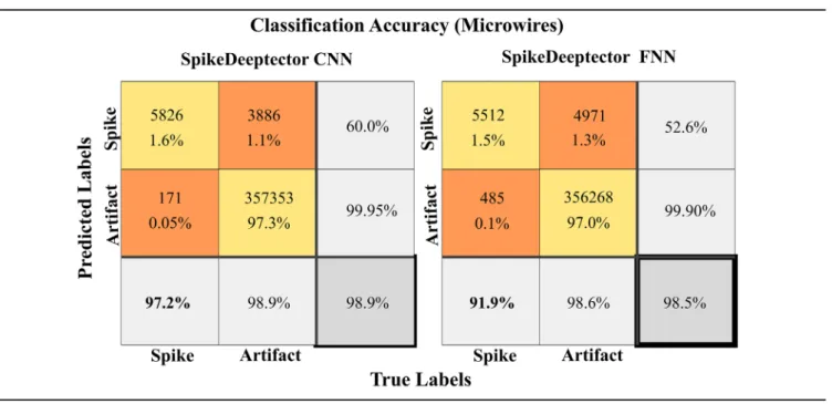
Table 4. Classification accuracy of trained models (SpikeDeeptector CNN and FNN) on the data collected from all patients implanted with microwires.
M Saif-ur-Rehman et al
containing neural data. The accuracy of SpikeDeeptector CNN and SpikeDeeptector FNN on the ‘spike’-labeled feature vectors is 94.6% and 92.6%, respectively, with SpikeDeeptector CNN outperforming SpikeDeeptector FNN by 2%. The evaluation performance of SpikeDeeptector CNN and SpikeDeeptector FNN on the ‘artifact’-labeled feature vectors is 97.9% and 98.6%, respectively. The overall acc-uracy of SpikeDeeptector CNN and SpikeDeeptector FNN is 96.7% and 96.5% (table 3).
The data distribution of patients implanted with microwires is even more unbalanced. Only 1.65% of the data represent feature vectors of class ‘spike’ and remaining 98.35% data rep-resent feature vectors of class ‘artifact’ (table 4). Accuracy of SpikeDeeptector CNN and SpikeDeeptector FNN on the ‘spike’ feature vectors is 97.2% and 91.9%. Here, SpikeDeeptector CNN outperforms SpikeDeeptector FNN with a difference in evaluation performance of 5.3%. The evaluation performance of SpikeDeeptector CNN and SpikeDeeptector FNN on the
‘artifact’ feature vectors is 98.9% and 98.6%. The overall accuracy of SpikeDeeptector CNN and SpikeDeeptector FNN is 98.9% and 98.6% (table 4).
The results in tables 3 and 4 show the classification acc-uracy of SpikeDeeptector CNN and SpikeDeeptector FNN on feature vectors constructed by considering all the recording sessions of Utah array and microwire patients. To evaluate the consistency of both models, we tested them on the feature vectors of all individual patients (see supplementary tables 12 and 13 (stacks.iop.org/JNE/16/056003/mmedia)) and on the feature vectors constructed exclusively from some specific channels of selected recording sessions (see supplementary tables 14–17). For a few recording sessions of different sub-jects, we also evaluated SpikeDeeptector CNN specifically at each channel, separately. For more details, see supplementary material: Reliability evaluation. The overall performance of SpikeDeeptector CNN and SpikeDeeptector FNN is compa-rable as shown in tables 3 and 4, supplementary tables 12 and
13. However, across all the recording sessions of individual patients, SpikeDeeptector CNN consistently outperforms SpikeDeeptector FNN on the feature vectors corresponding to
‘spike’ class (see supplementary tables 12 and 13). As a result, SpikeDeeptector CNN produces fewer false negatives, which are usually less desirable for neuroscientific analyses including online BCI. The results shown in supplementary material: Reliability evaluation also show that SpikeDeeptector CNN has successfully generalized across different data sources.
Impact of batch size
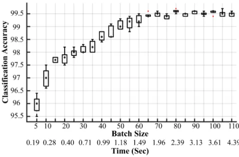
The box plots in figure 7 show the classification accuracy on the validation data Dva, when SpikeDeeptector CNN is trained
and evaluated ten times for each batch size. The time on the x-axis, which is also referred to as batch accumulation time (BAT), is the average time across all channels to accumulate waveforms equal to the corresponding batch size. The valida-tion accuracy remains consistent during most of the training trials at the corresponding batch size. However, there are few outliers at three different points (batch size =65, 80, 100). Based on Tukey’s rule, we considered the classification acc-uracy as an outlier if it is larger than the 3rd quartile (Q3) by at least 1.5 times the interquartile range (IQR), or smaller than 1st quartile (Q1) by at least 1.5 times the IQR.
Classification accuracy increases with increasing batch size (see figure 7), but BAT also increases. This trade-off between the classification accuracy and choosing the right batch size needed to be optimized. The classification accuracy with batch size 20 was 97.5% and reached 99.5% with batch size 65 before saturating. BAT is a critical factor in online decoding, however, and the time to construct a feature vector with batch size = 10 is 280 ms, which provides an acceptable classification of 97% with SpikeDeeptector CNN. Therefore, it is possible to con-struct a feature vector and track neural data from each channel during online decoding. On the other hand, for offline spike Figure 7. Impact of batch size on classification accuracy and time to construct feature vector ‘BAT (sec)’. Time on the x-axis shows the mean time (calculated on the dataset D) to accumulate the number of waveforms required by the corresponding batch size. The red dots are outliers (see text). The y -axis shows classification accuracy.
sorting there may be more leeway to choose a larger batch size, up to b = 65 where classification acc uracy saturates at 99.5% for SpikeDeeptector CNN. We chose b = 20 for the remaining analyses in this research work, but we note that the selection of batch size depends on the application.
Tracking of neural data
Units on a channel can vanish or new units can appear over the recording period. Another important aspect of this work is to track the presence or absence of neural units on channels continuously at runtime. We support this claim by employing
SpikeDeeptector CNN on the data of three different kinds of channels (figure 8), where the presence of a unit is stable, less stable or unstable. A fluctuation between presence and absence of neural units takes place occasionally in partially stable channels and much more frequently in unstable channels (shown in figure 8). On stable channels a unit is either present or absent during one complete recording session, as shown in figure 8. This result provides evidence that SpikeDeeptector CNN tracks the presence or absence of units comprehensively on all types of channels. Classifying a channel as stable or unstable can help determining which channels are useful, for example in BCI applications.
Figure 8. Performance of SpikeDeeptector CNN on tracking of neural data on different types of channels (stable, partially stable, unstable).
Figure 9. Randomly selected correctly classified examples. The events representing spikes are shown in blue and events presenting artifacts are shown in grey color.
M Saif-ur-Rehman et al
Figure 10. Randomly selected wrongly classified examples. The events representing spikes are shown in blue and events presenting artifacts are shown in grey color.
Table 5. Performance comparison of SpikeDeeptector CNN and SpikeDeeptector FNN with human experts across the selected recording session of subject U1.
Labeled by Total spike channels (out of 96) Total artifact channels (out of 96) False positives False negatives
SpikeDeeptector CNN 19 77 0 0 SpikeDeeptector FNN 18 78 0 1 Human expert 1 20 76 1 0 Human expert 2 16 80 0 3 Human expert 3 17 79 0 2 Human expert 4 17 79 1 3
Table 6. Performance comparison of SpikeDeeptector CNN and SpikeDeeptector FNN with human experts across the selected recording session of subject U2.
Labeled by Total spike channels (out of 96) Total artifact channels (out of 96) False positive False negative
SpikeDeeptector CNN 16 80 2 0 SpikeDeeptector FNN 14 82 2 2 Human expert 1 14 82 0 0 Human expert 2 12 82 0 2 Human expert 3 12 82 0 2 Human expert4 10 86 0 4
Table 7. Assigning reliability labels to the predicted outputs of SpikeDeeptector FNN and SpikeDeeptector CNN for the selected recording session of subject U1.
Reliable predictions: spike (correct, wrong) Reliable predictions: artifact (correct, wrong) Partially-reliable predictions: spike (correct, wrong) Partially-reliable predictions: artifact (correct, wrong) Unreliable predictions: spike (correct, wrong) Unreliable channel: artifact (correct, wrong) SpikeDeeptector CNN (18, 0) (77, 0) (1, 0) (0, 0) (0, 0) (0, 0) SpikeDeeptector FNN (15, 0) (77, 0) (2, 0) (0, 1) (1, 0) (0, 0) J. Neural Eng. 16 (2019) 056003
Visualization of correctly and wrongly classified examples
We selected a small subset of correctly and wrongly classified input for the sake of visualization and evaluation of the perfor-mance of SpikeDeeptector CNN. The examples were selected randomly from all 136 recording sessions and are shown in figures 9 and 10.
Performance comparison of SpikeDeeptector CNN with its counterparts
We assigned labels to channels based on the criteria explained in the methods section (see Assigning labels to channels). We then compared the classification accuracy of SpikeDeeptector CNN with SpikeDeeptector FNN and with four human experts (see tables 5 and 6). For this evaluation, we selected one recording session from each of the subjects with implanted Utah arrays (U1 & U2). Single Utah array contain 96 chan-nels. The evaluation performance of SpikeDeeptector CNN, SpikeDeeptector FNN and the other participants (human experts) is given in tables 5 and 6.
In the recording session selected from subject U1, SpikeDeeptector CNN performed slightly better than SpikeDeeptector FNN and all other participants (see table 5). SpikeDeeptector CNN predicted ‘spike’ channels and ‘ arti-fact’ channels with 100% accuracy. However, the average accuracy of human experts is 89.47% for correctly predicting
‘spike’ channels and 99.35% for correctly predicting ‘artifact’ channels. Here, SpikeDeeptector FNN predicts the ‘spike’ channels with 94.74% accuracy, and ‘artifact’ channels with 100%.
For the recording session from subject U2, SpikeDeeptector CNN achieved 2nd rank by making two mistakes (false posi-tives), as shown in table 6. It has predicted all ‘spike’ chan-nels correctly (100% accuracy), but wrongly predicted two
‘Artifact’ channels as ‘spike’ channels (false positives) (97.57% accuracy). Average human expert accuracy is 85.71% for ‘spike’ channels and 100% for ‘artifact’ chan-nels. SpikeDeeptector FNN predict the ‘spike’ channels with 85.71% accuracy, and the ‘artifact’ channels with 97.57% accuracy.
In order to compare SpikeDeeptector CNN and SpikeDeeptector FNN in terms of prediction reliability, we also assigned reliability tags (Assigning labels to chan-nels)to the above predicted outputs of both SpikeDeeptector CNN and SpikeDeeptector FNN as shown in tables 7 and 8. SpikeDeeptector CNN has a performance of 100% for the U1 dataset (table 5). More importantly, only one correct predic-tion has been assigned with label ‘Partially reliable prediction: Spike’, and all other correct predictions are reliable predic-tions (table 7). SpikeDeeptector FNN had one false negative for this same dataset (table 5), but more predictions were assigned with the tags ‘Partially reliable predictions: Spike’, Table 8. Assigning reliability labels to the predicted outputs of SpikeDeeptector FNN and SpikeDeeptector CNN for the selected recording session of subject U2.
Reliable predictions: spike (correct, wrong) Reliable predictions: artifact (correct, wrong) Partially-reliable predictions: spike (correct, wrong) Partially-reliable predictions: artifact (correct, wrong) Unreliable predictions: spike (correct, wrong) Unreliable predictions: artifact (correct, wrong) SpikeDeeptector CNN (14, 0) (80, 0) (0, 0) (0, 0) (0, 2) (0, 0) SpikeDeeptector FNN (12, 0) (80, 0) (0, 1) (0, 2) (0, 1) (0, 0)
Figure 11. Average accuracy of SpikeDeeptector CNN (with one standard deviation) across the channels labeled as ‘spike’ and ‘artifact’, on the data of two different recording sessions of microwire subjects, rethresholded at four different values starting from −4.5 to −3.5 times RMS of high pass filtered signal (cutoff frequency = 250 Hz), with step size of −0.25. (a) Average accuracy with one standard deviation of SpikeDeeptector CNN at different thresholding levels across the recording session of subject M1. For the recording session of M1, only one channel is labeled as ‘artifact’. Therefore, standard deviation is not shown. (b) Average accuracy with one standard deviation of SpikeDeeptector CNN at different thresholding levels across the recording session of subject M4. For the recording session of M4, only one channel is labeled as ‘spike’. Therefore, standard deviation is not shown.
M Saif-ur-Rehman et al
‘Partially reliable predictions: Artifact’ and ‘Unreliable pre-dictions: Spike’ (table 7). Similarly, the same trend can be seen for the dataset from subject U2 (table 8). Because the assigned reliability tag to the predicted output is an indication of the certainty of the prediction, partially reliable or unstable outcomes may need to be reviewed by the researcher. As an example, SpikeDeeptector CNN has two prediction mistakes (false positives) (see table 6) in the recording session of subject U2, which were assigned with tag of ‘Unreliable prediction’.
We show in tables 3 and 4, supplementary tables 12 and 13 that SpikeDeeptector CNN has classified fewer false nega-tives as compared to SpikeDeeptector FNN, across the data collected from all the subjects (Utah array and microwires). This prediction behavior of SpikeDeeptector CNN can also
be observed when predicting channel labels instead of fea-ture vectors (see tables 5 and 6). That means SpikeDeeptector CNN can consistently detect channels with label ‘spike’ more robustly as compared to SpikeDeeptector FNN. The results shown in tables 5 and 6 show that SpikeDeeptector CNN produces the least false negatives when compared with SpikeDeeptector FNN and even human experts. False nega-tives are potentially harmful because useful channels can be lost. In terms of false positives, SpikeDeeptector CNN and SpikeDeeptector FNN have comparable performance (tables 5 and 6). Finally, SpikeDeeptector CNN’s predictions are more reliable than SpikeDeeptector FNN’s (tables 7 and 8). For these reasons, SpikeDeeptector CNN is preferred over SpikeDeeptector FNN.
Figure 12. Average accuracy (with one standard deviation) of SpikeDeeptector CNN across the channels labeled as ‘spike’ and ‘artifact’, on the data of selected channels of two different recording sessions of Utah array subjects, rethresholded at four different values, starting from −4.5 times RMS of high pass filtered signal (cutoff frequency = 250 HZ) and stops at −3.5 times RMS of high pass filtered signal (cutoff frequency = 250 Hz), with step size of −0.25. (a) Average accuracy with one standard deviation of SpikeDeeptector CNN at different thresholding levels of subject U1 for both classes. (b) Average accuracy with one standard deviation of SpikeDeeptector CNN at different thresholding levels of subject U2 for both classes.
Table 9. Evaluation of the performance of SpikeDeeptector CNN at different sampling rates across the recording session of subject U1. Sampling rate (kHz) Total spike channel (out of 96) Total artifact channel (out of 96) False positive (out of 96) False negative (out of 96)
40 19 77 0 0 32 19 77 0 0 30 19 77 0 0 20 19 77 0 0 10 19 77 0 0 5 23 73 4 0 2.5 30 66 11 0
Table 10. Evaluation of the performance of SpikeDeeptector CNN at different sampling rates across the recording session of subject U2. Sampling rate
(kHZ) Total spike channel (out of 96) Total artifacts channel (out of 96) False positive (out of 96) False negative (out of 96)
40 16 80 2 0 32 16 80 2 0 30 16 80 2 0 15 16 80 2 0 10 16 80 2 0 5 18 78 3 0 2.5 28 68 13 0 J. Neural Eng. 16 (2019) 056003
Evaluation of robustness
We trained the model of SpikeDeeptector CNN with the data collected at 30 kHz sampling rate and a threshold setting of −4.5 times root-mean-square of the high pass filtered, full bandwidth signal with a cutoff frequency 250 Hz (see sec-tion Data collection for more details). To see if our results are robust, we evaluated the trained model of SpikeDeeptector CNN in three different ways.
1. Performance evaluation at different threshold settings. 2. Performance evaluation at different sampling rates. 3. Performance evaluation on a different species
(non-human primates (NHPs)) recorded using a different acquisition system.
Evaluation of SpikeDeeptector CNN at different threshold settings. To evaluate the performance of SpikeDeeptector CNN on different threshold settings, we selected two record-ing sessions of subjects implanted with microwires. For a fair evaluation, we selected two recording sessions of different subjects (M1 & M4) one with more channels corresponding to class ‘spike’ and the other with more channels corresponding to class ‘artifact’. Similarly, we selected two recording ses-sions, one from each subject (U1& U2) implanted with Utah arrays. From each Utah array recording session, we randomly selected four channels with true label ‘spike’ and other four channels with true label ‘artifact’. Then, we re-thresholded the data of all the selected recording sessions, starting from −4.5 times root-mean-square of the high pass filtered (cutoff fre-quency = 250 Hz) signal to −3.5 times root-mean-square of the high pass filtered (cutoff frequency = 250 Hz) signal, with a step size of −0.25. By reducing the threshold, we are allow-ing low amplitude noise in the feature vectors.
For the microwire array datasets (both recording sessions), SpikeDeeptector CNN produced comparable results at all threshold settings (figure 11). For subject M1, the minimum accuracy among both channel types at the most permissive threshold level is still more than 94% (figure 11(a)), meaning that all the channels can be labeled as reliable (see Assigning labels to channels). The performance of SpikeDeeptector CNN at different threshold values for data from subject M4 is similarly robust with a minimum average accuracy of more
than 90% (figure 11(b)). As a result, all the channels can be easily correctly classified with the highest defined reliability tag.
In case of Utah array recording sessions, overall perfor-mance of SpikeDeeptector CNN can be seen in figure 12. At lowest threshold setting, for both recording sessions the average accuracy of SpikeDeeptector CNN drops considerably on the channels corresponding to class ‘spike’ (see figure 12). For the recording session of subject U1, at lowest threshold setting, classification accuracy of SpikeDeeptector CNN on individual channels corresponding to class ‘spike’ is 95.66%, 76.71%, 89.59%, and 77.59%. As a result, all the channels can still be correctly classified, but according to defined criteria of assigning reliability tags, two channels (76.71%, 77.59%) will be assigned with the tag ‘Partially-reliable prediction: Spike’. Contrarily, performance of SpikeDeeptector CNN on most of the channels corresponding to artifacts is robust even at the lowest threshold setting as shown in figure 12(a). A Similar kind of behavior is observed in the recording ses-sion of subject U2, where, at lowest threshold settings, the classification accuracy of SpikeDeeptector CNN on the chan-nels corresponding to ‘spike’ is 82.51%, 84.36%, 82.79%, and 79.51%. Here, the performance of SpikeDeeptector CNN on the channels corresponding to ‘artifact’ remains unaffected as shown in figure 12(b).
Evaluation of SpikeDeeptector CNN at different sampling rates. Data acquisition systems for neural data operate at various sampling rates. The Blackrock Neural Signal Proces-sor runs with a maximum sampling rate of 30 kHz but there are systems with higher (Plexon Inc, OmniPlex at 40 kHz) and lower sampling rates. To test the performance of SpikeDeep-tector CNN at different sampling rates, we resampled our data (see tables 9 and 10). For the sake of consistency, we used the same recording sessions of subjects implanted with Utah arrays as before (Performance comparison of SpikeDeep-tector CNN with its counterparts). We first resampled the data to the desired sampling rate, and then applied interpola-tion to normalize the number of samples in each waveform back to 48 (the native resolution of our system). The perfor-mance of SpikeDeeptector CNN for different sampling rates is shown in tables 9 and 10. The performance of SpikeDeep-tector CNN remains stable until the data is downsampled to Table 11. Evaluation of the performance of SpikeDeeptector CNN and SpikeDeeptector FNN on two different publicly available datasets (CRCNS—PMD 1, CRCNS-PPC1).
Data set Recording hardware Electrode type Subject id Place of implantation
Ground truth: no. of spike channels Predicted label (SpikeDeeptector CNN): no. of spike channels Predicted label (SpikeDeeptector FNN): no. of spike channels CRCNS—PMD 1
Black-rock Utah array MM M1 45 44 40
CRCNS—PMD 1
Black-rock Utah array MM PMD 51 51 47
CRCNS—PMD 1
Black-rock Utah array MT PMD 34 32 24
CRCNS—PPC 1 Plexon Single microelectrodes
M Saif-ur-Rehman et al less than 10 kHz. Further reduction of the sampling rate
dras-tically reduced the performance of SpikeDeeptector CNN (see tables 9 and 10). A similar behavior has been reported in Navajas et al (2014), where the authors evaluated the perfor-mance of a spike sorting algorithm at different sampling rates.
Evaluation of SpikeDeeptector CNN on the data recorded from NHPs using different data acquisition systems. We evaluated the trained models of SpikeDeeptector CNN and SpikeDeeptector FNN on two publicly available labeled data-sets (CRCNS-PMD1 & CRCNS-PPC1) (table 11) (Shi et al 2013, Lawlor et al 2018). These datasets contain data from three NHPs, recorded from three different regions of the brain (M1, PMD, PPC). Some of the data were recorded using a dif-ferent recording system (Plexon, Inc.) and a difdif-ferent type of electrode (single microelectrodes). The dataset recorded with the Plexon system represents waveforms with 16 samples, so interpolation was required. Further details on the dataset can be found here (Shi et al 2013, Lawlor et al 2018). The perfor-mance of SpikeDeeptector CNN and SpikeDeeptector FNN is given in table 11. Here, SpikeDeeptector CNN performed much better than SpikeDeeptector FNN. However, both data-sets only contain data from channels where at least one unit is present.
Discussion
In this study, we presented two variants (SpikeDeeptector CNN, SpikeDeeptector FNN) of an algorithm we call
‘SpikeDeeptector’, which discriminates SUA and MUA chan-nels from chanchan-nels recording only noise. SpikeDeeptector works with data collected from different subjects, brain areas, recording sessions and different types of recording micro-electrodes. The evaluation performance of SpikeDeeptector CNN and SpikeDeeptector FNN on the data collected from eight subjects (see tables 3 and 4, supplementary tables 12 and 13) show that the trained models can generalize to new data. The overall performance of both models (SpikeDeeptector CNN& SpikeDeeptector FNN) is generally comparable. However, SpikeDeeptector FNN seems to be more prone to false negatives which is usually less desirable for neurosci-entific analyses, especially for online BCI. We showed that SpikeDeeptector CNN makes fewer mistakes on the fea-ture vectors representing spike (neural data) as compared to SpikeDeeptector FNN, across the data collected from all the subjects (Utah array and microwires) (tables 3 and 4, supplementary tables 12 and 13). SpikeDeeptector CNN performs similarly when predicting channels labels instead of feature vectors labels (tables 5 and 6). This finding sug-gests SpikeDeeptector CNN can detect neural channels more robustly compared to SpikeDeeptector FNN. SpikeDeeptector CNN produces the fewest false negatives across feature vec-tors and channels compared to SpikeDeeptector FNN and human experts (tables 5 and 6). SpikeDeeptector CNN also outperformed SpikeDeeptector FNN on the publicly available
NHP dataset (see table 11). Finally, SpikeDeeptector CNN’s predictions are more reliable as compared to SpikeDeeptector FNN’s (tables 7 and 8).
We showed some correctly and the wrongly classified examples (see figures 9 and 10). The correctly classified examples confirm that SpikeDeeptector CNN properly dis-tinguished neural data from artifacts. Some of the wrongly classified examples are very difficult even for human experts to classify, e.g. events representing spikes in figure 10 (top left) and some of the events representing artifacts (figure 10; bottom right).
We trained the SpikeDeeptector CNN model on data col-lected at 30 kHz sampling rate and a threshold setting of −4.5 times the root-mean-square of the noise in the high pass fil-tered signal (see section Data collection for more details). We evaluated the robustness of our algorithm to different sam-pling rates, electrode types, threshold settings, and acquisition systems. The results in Evaluation of robustness show that SpikeDeeptector CNN consistently performed best. We also showed that our algorithm runs competitively across species using different acquisition systems and implanted with dif-ferent kinds of electrodes.
Over the years many other studies on automatic spike detec-tion have been published (Kim and McNames 2007, Ji et al 2011, Wen-Jyi et al 2014, Gerhard et al 2018). In Kim and McNames (2007), the authors proposed a method to detect spikes called ‘adaptive template matching’. This proposed method detects the spike events by processing the input signal
x(n) in four different stages. In the first stage the inputs signal x(n) is enhanced to detect peaks by calculating the instanta-neous powerxp(n) of x(n), and by applying low pass filter with a cutoff frequency equal to the maximum firing rate fmax of the
neurons, which must be specified by the user. In the second stage, the estimation of probability density function (PDF) of similarity maxima is required to estimate the threshold. In the third stage, the detected spikes are used to estimate the template and to measure a degree similarity between the input signal template. The signals recorded from the brain are highly nonstationary (time varying signal) and the placement of implanted electrodes can also change with the passage of time. Therefore, it is possible that the same implanted elec-trode records the activity of different sources (neurons) in two different recording sessions, which invalidates the estimated parameters of the algorithm proposed in Kim and McNames (2007). Another drawback of adaptive template matching is that it estimates a separate model for each electrode. State-of-the-art microelectrode arrays contain hundreds of channels and would require hundreds of parameter models, which might then become invalidated in subsequent recording sessions. Adaptive template matching also requires some input from the user, e.g. neuronal firing rate, to estimate the parameters, which is not the case in our proposed method.
There are some studies in which supervised machine learning methods are used to detect and sort spikes (Oghalai et al 1994, Horton et al 2007, Yang et al 2017). However, none of these studies have investigated the generalization quality
of machine learning across different recording sessions, sub-jects, and types of implantable electrodes.
SpikeDeeptector has several other useful applications. During online decoding in invasive brain computer interface (BCI) systems, feature vectors are often constructed from threshold crossing events (Fraser et al 2009, Koyama et al 2009, Aflalo et al 2015, Klaes et al 2015). With SpikeDeeptector threshold crossing events not representing neuronal activity can be easily discarded. As a result, more meaningful feature vectors can be constructed. Moreover, it has also been shown in previous BCI studies that units disappear or appear with the passage of time (Sanchez et al 2004, Moritz and Fetz 2011, Lebedev 2014). By employing SpikeDeeptector, one can auto-matically track the presence or absence of single unit activity at runtime (see Tracking of neural data).
Most existing spike sorting methods operate either manu-ally or semi-automaticmanu-ally (Lewicki 1998, Einevoll et al 2012, Marre et al 2012, Quiroga 2012). Many of them follow a pro-cess pipeline, which typically includes a step of feature reduc-tion, either for visualizareduc-tion, for feature vector extraction for clustering algorithms, or for both. In such manual spike sorting methods, human intervention is required for channel selection and for clustering. The latter is done by examining the features in a 2D projection and manually defining clus-ters. Here, SpikeDeeptector can be employed to reduce the time and effort needed at the first stage by automatically dis-carding the channels that contain only artifacts. Another way of manual spike sorting is the hoop technique, where different hoops (thresholds) are defined manually at each channel of implanted array to sort spikes from multiple neurons. The process of defining hoops is time intensive and has to be adjusted as signals change over time, either acutely (within session) or chronically (across sessions). Typically, threshold settings for hoop sorting cannot simply be reused in consecu-tive recording sessions. It is possible that many channels of the implanted array do not record neural data at all. Here, SpikeDeeptector can be employed to reduce the time and effort needed in the first stage of spike sorting by automati-cally discarding channels that contain only artifacts, therefore considerably reducing human effort. Hoop sorting can then be applied on the remaining channels.
In semi-automatic spike sorting, clustering is done auto-matically, but the user must curate in order to decide which clusters to reject and which clusters to accept (Hill et al 2011, Kadir et al 2014, Rossant et al 2016). SpikeDeeptector can automatically promote ‘spike’ clusters and reject ‘artifact’ clusters (see Batch size). However, if the clustering algorithm wrongly merged two distinct units, or a unit and artifact, or if the clustering algorithm wrongly split a unit into two dis-tinct clusters, the current version does not provide a solution to manipulate clustering.
SpikeDeeptector is a supervised learning algorithm and needs labeled data for training. We carefully labeled the data as explained in Data labeling. However, ground truths are based on human judgment and could contain errors.
However, this is not unusual since all big data sets in the field of computer vision (image net, MNIST, CIFAR-100) are hand labeled and could contain errors. Nonetheless, deep learning algorithms usually perform well on test data even though the possibility of ground truth errors cannot be excluded. We showed in the result section Performance comparison of SpikeDeeptector CNN with its counterparts that the perfor-mance of SpikeDeeptector is comparable to different human experts.
Source separation is another important issue that still needs to be addressed. Although many methods exist to solve this issue, very few of them offer fully automated spike sorting (Chung et al 2017, Grossberge et al 2018, Hossein Nadian et al 2018) and none of them offer a universal fully automated spike sorter. We aim to extend the SpikeDeeptector algorithm so that it will not only determine the presence or absence of neural data on the channel, but also detect and track individual neural sources, universally.
The current version of SpikeDeeptector detects and tracks channels containing neural data recorded from multiple human subjects and one nonhuman primate. In the future we also want to extend the scope of SpikeDeeptector to data from different spike types (excitatory, inhibitory) (Becchetti et al 2012), cell types, and species (rat, cat).
Conclusions
In this study, we propose a novel algorithm called SpikeDeeptector to detect and track channels containing neural data from implanted electrodes, automatically and uni-versally. To the best of our knowledge, there is no method that can universally and automatically extract channels containing neural data. We supported our claim by evaluating our method on the data collected from six epileptic patients implanted with depth electrodes and two tetraplegic patients implanted with two Utah arrays. SpikeDeeptector has potential for online and offline automatic spike sorting in BCI applications. The sig-nificance of SpikeDeeptector could potentially increase when microelectrode arrays with larger sizes become available. As a result, SpikeDeeptector could be envisioned to become an integral part of data analysis of single cell recordings. In the future, we aim to extend the scope of SpikeDeeptector to the data collected from even more different species and different types of neural cells. We also intend to extend our method so that it detects and tracks every present neural source on the channel.
Acknowledgments
This study was funded by the Deustche Forschungsgemein-schafts (DFG, German Research Foundation) under proj-ects number KL 2990/1-1—Emmy Noether Program, and 122679504—SFB 874. We would also like to acknowledge Nina Misselwitz for providing clinical support during the recording sessions of the epilepsy patients.