Test Problems for Large-Scale Multiobjective and
Many-Objective Optimization
Ran Cheng, Yaochu Jin, Fellow, IEEE, Markus Olhofer and Bernhard Sendhoff, Senior Member, IEEE
Abstract—The interests in multi- and many-objective
optimiza-tion have been rapidly increasing in the evoluoptimiza-tionary computaoptimiza-tion community. However, most studies on multi- and many-objective optimization are limited to small-scale problems, despite the fact that many real-world multi- and many-objective optimization problems may involve a large number of decision variables. As has been evident in the history of evolutionary optimization, the development of evolutionary algorithms for solving a particular type of optimization problems has undergone a co-evolution with the development of test problems. To promote the research on large-scale multi- and many-objective optimization, we propose a set of generic test problems based on design principles widely used in the literature of multi- and many-objective optimization. In order for the test problems to be able to reflect challenges in real-world applications, we consider mixed separability between decision variables and non-uniform correlation between decision variables and objective functions. To assess the proposed test problems, six representative evolutionary multi- and many-objective evolutionary algorithms are tested on the proposed test problems. Our empirical results indicate that although the compared algorithms exhibit slightly different capabilities in dealing with the challenges in the test problems, none of them are able to efficiently solve these optimization problems, calling for the need for developing new evolutionary algorithms dedicated to large-scale multi- and many-objective optimization.
Index Terms—Evolutionary algorithms, multi-objective
opti-mization, many-objective optiopti-mization, large-scale optiopti-mization, test problems
I. INTRODUCTION
M
ULTI- and many-objective optimization problems in-volve more than one conflicting objective to be opti-mized simultaneously, which can be formulated as follows:min
x f(x) = (f1(x), f2(x), ..., fM(x))
s.t. x∈X (1)
where X ⊆ Rn is the decision space with x = (x1, x2, ..., xn) ∈ X being the decision vector. Due to the
conflicting nature of the objectives, a set of optimal solutions representing the trade-off between different objectives, termed Pareto optimal solutions, can be achieved. The Pareto optimal solutions are known as the Pareto front (PF) in the objective space and the Pareto set (PS) in the decision space. Usually, multi-objective optimization problems (MOPs) refer to those Ran Cheng and Yaochu Jin are with the Department of Computer Science, University of Surrey, Guildford, Surrey, GU2 7XH, United Kingdom (e-mail: [email protected]; [email protected]). Y. Jin is also with the College of Information Sciences and Technology, Donghua University, Shanghai 201620, P. R. China. (Corresponding author: Yaochu Jin)
Markus Olhofer and Bernhard Sendhoff are with the Honda Research Institute Europe, 63073 Offenbach, Germany (e-mail: {markus.olhofer;bernhard.sendhoff}@honda-ri.de).
with two or three objectives, while those with more than three objectives are known as many-objective optimization problems (MaOPs) [1]–[4].
Evolutionary algorithms (EAs), which are population-based, are well suited for solving MOPs and MaOPs as they can obtain a solution set in one single run [5]. In general, multi-objective evolutionary algorithms (MOEAs) can be catego-rized into three groups, including dominance based meth-ods [6]–[8], decomposition based methmeth-ods [9]–[11], and per-formance indicator based methods [12], [13]. In addition to the conventional MOEAs, a few MOEAs dedicated to solving MaOPs have recently been developed [14]–[19].
To evaluate the performance of various MOEAs, several test suites have been designed for empirical studies. Among many others, the ZDT test suite [20] and DTLZ test suite [21], [22] are the most widely used ones.
The ZDT test suite is one of the most popular test suites in the multi-objective optimization literature [20]. Based on the generic design principles proposed by Deb in [23], the test problems in the ZDT suite are constructed by introducing three basic functions, including a distribution function f1, a
distance function g and a shape function h, where function f1 is designated to test the ability of an MOEA to maintain
diversity along the PF, function g is meant for testing the ability of an MOEA to converge to the PF and functionhfor defining the shape of the PF. There are six test problems in the ZDT test suite, five of which (ZDT1 to ZDT4, ZDT6) are real-coded and one (ZDT5) is binary-real-coded. Different ZDT test problems have different characteristics. Specifically, ZDT3 has a disconnected PF, which is partly convex and partly concave; ZDT4 contains a large number of local PFs; ZDT6 has a non-uniform fitness landscape, which causes a biased distribution of the Pareto optimal solutions along the PF. However, despite its immense popularity, the ZDT test suite has a significant limitation, i.e., all test problems are bi-objective.
To address the limitation of the ZDT test suite (as well as many other bi-objective test problems), Deb et al. proposed another test suite, i.e., the DTLZ test suite [21], [22], in which the test problems are scalable to have any number of objectives. There are nine test problems in the DTLZ test suite, each of which is constructed with the same design principle, where the firstM−1decision variables define the PF, while the rest decision variables specify the convergence property. The DTLZ test suite has many unique characteristics. For instance, the fitness landscape of DTLZ1 and DTLZ3 contain a large number of local PFs; the distribution of the Pareto optimal solutions of DTLZ4 is highly non-uniform; the PFs of DTLZ5 and DTLZ6 are a degenerate curve; DTLZ7 has a disconnected
PF; and DTLZ8 and DTLZ9 are constrained problems. One significant contribution of the DTLZ test suite is the proposal of a generic design principle for constructing test problems that are scalable to have any number of objectives, as well as decision variables.
Some variants of the DTLZ test suite have also been devel-oped. To assess the performance of MOEAs on highly scaled problems [16], Deb et al. proposed a method to scale the value of each objective function to a different range. In [24], some constrained DTLZ problems have been suggested to verify the constraint handling capability of MOEAs. However, in spite its immense popularity, the DTLZ test suite still has some shortcomings. For example, it doses not take into account some important characteristics commonly seen in the real-world problems, such as variable linkage and variable separability. In this work, separability refers to the correlation relationship between the decision variables in the entire decision space, while variable linkage is used to characterize the relationship between the decision variables of Pareto optimal solutions.
To remedy the shortcomings of the DTLZ test suite, Huband et al. proposed another test suite, i.e., the WFG test suite [25], [26]. The WFG test suite has incorporated a variety of important characteristics that widely exist in real-world problems. To construct a test problem, it only requires to specify a shape function, which determines the PF, and a transformation function, which describes the fitness landscape. In this test suite, WFG1, WFG7 and WFG9 have biased PFs; WFG5 and WFG9 have deceptive fitness landscapes; WFG2, WFG3, WFG6, WFG8 and WFG9 have non-separable fitness landscapes. Since these test problems are also scalable to have any number of objectives, the WFG test suite becomes another prevalent benchmark for many-objective optimization, in addition to the DTLZ test suite.
Apart from the above three general-purpose test suites, test problems have also been constructed to include some specific characteristics. In [27], Okabe et al. have proposed some design principles for constructing test problems with an arbitrarily complex PS, which were generalized in [28]. More recently, Saxena et al. have extended the test problems with complex PSs for many-objective optimization [29]. Other modified ZDT and DTLZ test problems by introducing linear or nonlinear variables into decision variables can be found in [30] [31]. While the test problems discussed above are static, dynamic multi-objective optimization test problems have also been proposed in [32], where the PFs and/or PSs change over time. Some variants of these test problems can also be found in [33], [34].
However, in spite of the various test problems above, none of them is designed for large-scale optimization by explic-itly taking considering different characteristics of decision variables, even if they are theoretically scalable to have any number of decision variables. Despite the fact that large-scale optimization has attracted much attention in single-objective optimization [35]–[37], little work has been reported on large-scale multi- and many-objective optimization with few exceptions [38]–[40]. This can partly be attributed to the lack of large-scale multi- and many-objective optimization test problems, unlike the rich literature on large-scale
single-objective optimization [41]–[44].
This work aims to propose a set of test problems for large-scale multi- and many-objective optimization. The main new contributions of this work can be summarized as follows:
1) Following a few basic design principles, new considera-tions have been introduced in constructing test problems for large-scale multi- and many-objective optimization, including non-uniform correlations between decision variables and objective functions, and mixed separability in the fitness landscape. To the best of our knowledge, this is the first time that such properties have been taken into account in multi- and many-objective test problems. 2) A generic method for defining correlations between the decision variables and the objective functions has been proposed. With a correlation matrix, any relationship between decision variables and objectives can be easily defined.
3) Based on the proposed design principles and consid-ered characteristics, nine large-scale multi- and many-objective test problems (LSMOPs for short hereafter) have been constructed.
The remainder of this paper is organized as follows. Section II introduces a few fundamental concepts in large-scale opti-mization. Section III and Section IV present the basic design principles and problem characteristics, respectively. On the ba-sis of these, nine LSMOPs are proposed in Section V. Section VI presents the empirical results of six selected MOEAs for multi- and many-objective optimization on the proposed test problems. Finally, Section VII draws the conclusion.
II. BACKGROUND
In this section, we first go through a few basic concepts in large-scale optimization, such as separability and non-separability, followed by a brief review of some representative test suites for large-scale single-objective optimization.
A. Basic Concepts in Large-Scale Optimization
Large-scale optimization generally refers to the solution of optimization problems that involve hundreds or even thousands of decision variables [45]–[47]. As pointed by Weise et al. in [48], several factors make large-scale optimization problems extremely difficult. For example, with the increase of the num-ber of decision variables, the volume of search space grows exponentially, and the complexity of the fitness landscape increases rapidly as well. Nevertheless, the major difficulty comes from the interactions between decision variables, often known as the non-separability. To be specific, an objective functionf(x)is said to be separable with respect to a decision variablexk if the following condition is fulfilled [35]:
f(x)< f(x′)⇒f(y)< f(y′) (2) where x = [x1, ..., xk, ..., xn], x′ = [x′1, ..., x′k, ..., x′n],
y = [y1, ..., xk, ..., yn] and y′ = [y1′, ..., x′k, ..., y′n] are four
different decision vectors. Otherwise, f(x) is considered to be non-separable with respect to xk, which means that xk
has interactions with one or more other decision variables. Specially, if the decision variables only interact with some
(rather than all) of the other decision variables, the objective function f(x)is known as a partially separable function.
Several important observations can be made with regard to separability, non-separability and partial separability [44], which are listed below.
A decision variablexk can be optimized independently iff
the objective functionf(x)is separable with respect to it:
argmin x f(x) = argmin xk f(x),argmin ∀xj,j6=k f(x) ! (3)
The decision variables can be optimized component-wise independently iff an objective functionf(x)is partially sepa-rable: argmin x f(x) = argmin x1 f(x1, ...), ...,argmin xm f(...,xm) (4) where x1, ..., xm are disjoint sub-vectors of x, and the interactions only exist among decision variables inside each sub-vector, but the decision variables in different sub-vectors do not interact with each other.
B. Benchmark Test Suites for Large-Scale Single-objective Optimization
The first benchmark suite for large-scale single-objective optimization was proposed by Tang et al. in the CEC’2008 special session and competition on large-scale global opti-mization [41]. This suite is now known as the CEC’2008 suite consisting of seven test problems. This is the first attempt to explicitly include the characteristics of separability and non-separability into test problems for large-scale optimization. However, a major weakness of this test suite is that the problems are designed to be either fully separable or fully non-separable, which are two extreme cases of most real-world problems.
The CEC’2008 test suite was extended by Tang et al. to construct the CEC’2010 test suite [42]. The major contribution of CEC’2010 test suite is the proposal of a modularity based design principle, which divides the decision variables into different subcomponents, and the separability of each subcom-ponent is independent. Consequently, the test problems can be fully separable, partially separable or fully non-separable by combining separable and non-separable subcomponents. The CEC’2010 test suite has motivated the development of techniques such as random grouping [35], cooperative co-evolution [36], and differential grouping [49], which are used to detect interactions between groups of decision variables and solve them in a divide-and-conquer manner.
The CEC’2013 test suite has been proposed on the basis of the CEC’2010 test suite to include a few new charac-teristics [43]. First, some subcomponents in the CEC’2013 test suite are overlapped, while the subcomponents of the decision variables in the CEC’2010 test suite are completely independent. Second, the size of all the subcomponents is fixed in the CEC’2010 test suite, while in the CEC’2013 test suite, the subcomponents are of different sizes, such that they have non-uniform contributions to the objective function.
III. DESIGNPRINCIPLES
In the design of the proposed test problems, we follow four basic principles as suggested in [21] and [26]:
1) The test problems can be generated with a uniform design formulation.
2) The test problems should be scalable to have an arbitrary number of objective functions.
3) The test problems should be scalable to have any number of decision variables.
4) The exact shapes and locations of the PFs are known. The above four principles guarantee a good extensibility and generality of the test problems. To fulfil these four design principles, the following uniform design formulation is adopted: f1(x) =h1(xf)(1 +g1(xs)) f2(x) =h2(xf)(1 +g2(xs)) ... fM(x) =hM(xf)(1 +gM(xs)) (5)
where f1 to fM are the objective functions, xf = (x1, ..., xm−1) is the first part of the decision vector and xs = (xm, ..., xn) is the other part, functions h1, ..., hM
to-gether define the shape of the PF, known as the shape functions hereafter, and functionsgidefine the fitness landscape, known
as the landscape functions hereafter.
If we denote F(x) = [f1(x), ..., fM(x)], H(xf) = [h1(xf), ..., hM(xf)], and G(xs) = diag(g(xs), ..., g(xs)),
(5) can be rewritten as:
F(x) =H(xf)(I+G(xs)), (6) whereI is an identity matrix,H(xf) is known as the shape matrix andG(xs)is known as the landscape matrix.
Given a problem as formulated by (6), the optimization target is to find the PS, denoted as x∗ = (xf∗,xs
∗), such that
G(xs∗) =O andF(x∗) =H(x
f
∗). Therefore, by using such a design formulation, H(xf)is able to test the ability of an algorithm to achieve diverse solutions along the PF, andG(xs)
is able to test the ability of an algorithm to converge to the PF.
Since the motivation of this work is to introduce some important characteristics into large-scale fitness landscapes of the proposed test problems, we focus on the design ofG(xs),
which defines the fitness landscape. While forH(xf), which
defines the shape of the PF, we simply refer to the existing definitions in [21]. In the following section, we will introduce the detailed characteristics of the proposed test problems with respect to the design ofG(xs).
IV. TESTPROBLEMCHARACTERISTICS
There are four main characteristics of the proposed test problems with regard to the design of the landscape matrix
G(xs)as described in (6):
1) The decision variables are non-uniformly divided into a number of groups.
2) Different groups of decision variables are correlated with different objective functions.
3) The decision variables have mixed separability. 4) The decision variables have linkages on the PSs. Characteristic (1) and characteristic (3) follow the design principles of large-scale single-objective optimization prob-lems, as recommended in [44]; characteristic (4) follows the suggestions in [27] and [28] to take into consideration the variable linkages on the PSs, while characteristic (2) is to reflect the scenarios in real-world conceptual design [50]–[52].
A. Non-uniform Grouping of Decision Variables
The decision vector xs is non-uniformly divided into M groups as follows:
xs= (xs1, ...,xsM), (7)
where M is the number of objectives, and
M
P
i=1
|xsi|=|xs|=
ns, with ns being a predefined parameter that specifies the
total number of decision variables inxs. Moreover, each group
further consists of a number of nk subcomponents:
xsi = (xsi,1, ...,x
s
i,nk), (8)
wherenk is a predefined parameter that specifies the number
of subcomponents in each group of decision variables. To guarantee that the non-uniform group sizes are constant in different independent runs, we propose a chaos-based pseudo random number generator:
|xsi|=⌈ri×ns⌉, ri= ci PM i=1ci (9) with ci= ( α×ci−1×(1−ci−1), i >1 α×c0×(1−c0), i= 1 , (10)
whereαandc0are parameters for the logistic map1presented
by (10). In this way, it is guaranteed that the pseudo random number list r1, ..., rM is fixed and satisfiesP
M
i=1ri= 1, such
that the random group sizes from |xs
1|, ...,|xsM| are fixed as
well, as long as the same settings of α andc0 are given. In
this work,α= 3.8andc0= 0.1are recommended. One thing
to be noted is that since the ceiling function (⌈·⌉) has been used in (9) to obtain integer numbers, the total number of decision variables in xs after non-uniform grouping can be slightly larger than the predefined parameterns.
B. Different Correlations between Variable Groups and Ob-jective Functions
Theoretically, a decision variable can be correlated with any (one or multiple) objective functions. For simplicity, we correlate a group of decision variables with a group of
1Logistic map is an archetypal example to show how chaotic behavior can
arise from very simple non-linear dynamical equations [53].
objective function(s), where the correlations can be described using a correlation matrix:
C= c1,1 c1,2 · · · c1,M c2,1 c2,2 · · · c2,M .. . ... . .. ... cM,1 cM,2 · · · cM,M (11)
whereci,j = 1 means that objective function fi(x) is
corre-lated with the decision variables in group xsj, and ci,j = 0
otherwise.
Correspondingly, if we denote C = (c1, ...,cM)⊤, the
landscape matrixG(xs)in (6) can be presented as:
G(xs) =diag(c1¯g1(xs), ...,cM¯gM(xs)) (12) with ¯ gi(xs) = (¯gi(xs1), ...,g¯i(x s M))⊤, (13) wherei= 1, ..., M,xs
i is thei-th group of decision variables,
as defined in (7), andg¯1 tog¯M are basic functions that define
the fitness landscape for each objective function.
If we substitute the landscape matrixG(xs)in (6) with (11)
to (13), the formulation of (5) can be rewritten as:
f1(x) =h1(xf)(1 + M X j=1 c1,jׯg1(xsj)) ... fi(x) =hi(xf)(1 + M X j=1 ci,jׯgi(xsj)) ... fM(x) =hM(xf)(1 + M X j=1 cM,j×g¯M(xsj)) (14) wherei= 1, ..., M.
Thus, the correlations between the decision variables and the objective functions can be fully specified using the correlation matrix C, where the correlations can be either separable or overlapped.
C. Mixed Separability
As pointed in [44], since real-world problems are rarely fully separable or non-separable, it is important to introduce mixed separability into test problems for large-scale optimiza-tion.
Specifically, mixed separability can be realized by applying different basic fitness landscape functions ¯gi in (14), which
are some single-objective optimization functions of different types of separability.
D. Variable Linkages on PSs
The variable linkages on PSs is a kind of important charac-teristic to be taken into consideration in the design of multi-objective optimization test problems [27], [28], [54]. The main motivation of introducing variable linkages is to consider a more general distribution of the Pareto optimal solutions,
making it more challenging for MOEAs to achieve diverse solutions.
Generally, variable linkages can be defined using a linkage function:
xs←L(xs), (15)
wherexsconsists of the decision variables that define the PS, andLis the linkage function that defines the linkages between the variables in xs.
V. THEPROPOSEDTESTPROBLEMS
۴(ܠ)
۶(ܠ) ۵(ܠ௦)
݄ଵ(ܠ),… ݄ெ(ܠ) ݃ҧଵ(ܠ௦),…݃ҧெ(ܠ௦) ۱ ࡸ(ܠ௦)
Fig. 1. The structure of the proposed test problems. A test problemF(x) consists of a shape matrixH(xf)and a landscape matrixG(xs), which are
further composed of four components: a group of shape functionshi(xf), a
group of landscape functionsg¯i(xs), a correlation matrixC, and a linkage
function L(xs), withi= 1, ..., M.
As formulated in (6), generally, a test problemF(x)consists of two parts: the shape matrixH(xf)and the landscape matrix
G(xs), where xf and xs are the first part and second part
of the whole decision vector x, respectively, and the Pareto optimal solution set ofF(x)is defined as:
(
PS:x∗ = (xf∗,xs∗)
PF:H(xf∗) , (16)
which satisfies G(xs
∗) =O, such thatF(x∗) =H(xf∗). More specifically, for i = 1, ..., M, H(xf) consists of a
group of shape functionshi(xf), as formulated in (5);G(xs)
consists of a group of landscape functions¯gi(xs)together with
a correlation matrixC, as formulated in (12). In addition, the variable linkages on the PSs are defined by a linkage function L(xs), as described in Section IV-D. An illustration of the structure of the proposed test problems can be found in Fig. 1. Therefore, to define a test problem F(x), it is required to specify the following four basic components:hi(xf),g¯i(xs),
C andL(xs).
This section first presents some instances of the four basic components that constitute the test problems. Afterwards, nine test problems are constructed based on the combinations of the instances of each component2.
A. Instances of the Shape Functions hi(xf)
In our design principles, the PF of a test problem is defined by a group of shape functions hi(xf). In general, the basic
2The Matlab code of the proposed test problems can be downloaded from:
http://www.soft-computing.de/jin-pub year.html
TABLE I
THE PROPERTIES OF THE BASIC SINGLE-OBJECTIVE OPTIMIZATION PROBLEMS.
Problem Modality Separability
η1: Sphere function Unimodal Separable η2: Schwefel’s problem 2.21 Unimodal Non-separable
η3: Rosenbrock’s function Multi-modal Non-separable η4: Rastrigin’s function Multi-modal Separable η5: Griewank’s function Multi-modal Non-separable
η6: Ackley’s function Multi-modal Separable
geometrical structure of a PF can be either linear, convex, concave, while the basic distribution property of a PF can be either continuous, disconnected or degenerate. As suggested in [26], a PF can be made complicated by mixing different basic geometrical structures and distribution properties.
Nevertheless, since this work focuses on the properties of the decision variables, here we only provide three basic instances of PF, including a linear PF (denoted as H1), a
convex PF (denoted as H2) and a disconnected PF (denoted
asH3) , which are taken from the DTLZ test suite suggested
in [21]. To be specific, the linear PF is almost the same as that in DTLZ1, except that each objective is normalized to [0,1]
instead of [0,0.5], while the convex PF and the disconnected PF are exactly the same as those of DTLZ2 and DTLZ7, respectively. The detailed definitions of the three instances can be found in Supplementary Materials I.
B. Instances of the Basic Landscape Functions¯gi(xs)
In general, the basic landscape functions ¯gi(xs) can be constructed based on any (combinations of) single-objective functions. In the proposed test suite, we suggest six basic single-objective optimization problems for the construction of basic landscape functions ¯gi(xs), including the Sphere func-tion, the Schwefel’s problem 2.21, the Rosenbrock’s funcfunc-tion, the Rastrigin’s function, the Griewank’s function, and the Ackley’s function, denoted as η1 to η6, which are not only
widely adopted as test functions to assess the performance of large-scale optimization algorithms [35]–[37], [55], but also commonly used to construct large-scale optimization test problems [41]–[43]. The properties of these functions are summarized in Table I and the detailed definitions can be found in Supplementary Materials II.
It should be noted that although all the six basic single-objective functions have a fixed global optimum (except that the global optimum ofη3isx∗=1, the global optimum of the
other five functions is x∗ =0), the Pareto optimal solutions have been shifted to different positions in the decision space by applying the variable linkages to be introduced in Section V-D. To ensure that the objective function values are not too distant from the true PFs, the values of the single-objective functions are further normalized by dividing the length of the decision vectors as follows:
¯ gi(xsi) = 1 nk nk X j=1 η(xsi,j) |xs i,j| , (17)
whereηis one of the basic functions fromη1toη6as listed in
Table I, andxs
i,jdenotes thej-th subcomponent in the variable
group xs i.
In addition, since the test problems are proposed for both multi- and many-objective optimization, to makeg¯i(xi
s)
scal-able to any number of objectives, we divide ¯gi(xi
s) into two groups: ( ¯ gI(xs i) ={¯g2k−1(xsi)}, ¯ gII(xs i) ={¯g2k(xsi)}. (18) where k = 1, ...,⌈M/2⌉, ¯gI(xs i) and g¯ II(xs i) contain
land-scape functions with odd and even indices, respectively. In this way, given an arbitrary objective number M, the fitness landscapes can be defined by relating ¯gI(xs
i)andg¯II(xsi)to
one of the basic functions amongη1 toη6according to (17).
C. Instances of the Correlation Matrix C
Generally, the correlation matrix C can be arbitrarily de-fined to specify the correlation relationship between the vari-able groups and the objective functions. Here we present three typical instances to be used in the proposed test problems.
1) Separable Correlations: C1= 1 0 · · · 0 0 1 · · · 0 .. . ... . .. ... 0 0 · · · 1 (19) ( ) i f x fM( )x s i x … 1( ) f x … … 1 s x … s M x
Fig. 2. The separable correlations between the variable groups and the objective functions.
The separable correlations between the variable groups and the objective functions can be described by an identity matrix
C1, where the elements on the diagonal are set to1 and all
others are set to 0. In this way, each objective function is correlated with only one variable group. An illustration of the separable correlations is given in Fig. 2.
2) Overlapped Correlations: C2= 1 1 0 · · · 0 0 1 1 0 ... .. . 0 . .. . .. 0 .. . 0 0 1 1 0 · · · 0 1 (20)
The overlapped correlations between the variable groups and the objective functions are presented by a matrix C2,
where the neighboring elements C2(i, i+ 1) are set to 1 in
addition to the elements on the diagonal, withi= 1, ..., M−1,
s M x ( ) i f x fM( )x s i x 1 s i x … 1( ) f x … … 2 s x 1 s x …
Fig. 3. The overlapped correlations between the variable groups and the objective functions.
and the other elements are set to0. In this way, each objective function has an overlapped correlation with two neighboring variable groups at the same time. Fig. 3 presents an illustrative example of the overlapped correlations.
3) Full Correlations: C3= 1 1 · · · 1 1 1 · · · 1 .. . ... . .. ... 1 1 · · · 1 (21) ( ) i f x fM( )x s i x … 1( ) f x … … 1 s x … s M x
Fig. 4. The full correlations between the variable groups and the objective functions.
The full correlations between the variable groups and the objective functions are presented by a matrixC3, where all the
elements are set to be1. In this way, each objective function has a full correlation with all the variable groups at the same time. The full correlation relationship is visualized in Fig. 4. D. Instances of the Linkage FunctionL(xs)
The general design principle of the linkage functions is similar to that in [30] and [31], where each decision variable in xs (denoted as xs
i, i = 1, ..., ns) is linked with the first
decision variable in xf, i.e., xf
1. In this work, we consider
both linear and nonlinear variable linkages, which will be elaborated in the following.
1) Linear Variable Linkage: L1(xs) = (1 + i |xs|)×(x s i −li)−x f 1×(ui−li), (22) 2) Nonlinear Variable Linkage:
L2(xs) = (1 + cos(0.5π i |xs|))×(x s i −li)−x f 1×(ui−li), (23) where ui and li is the upper and lower boundaries of
decision variable xs
i. In the proposed test problems, as will
be presented later on in Section V-B, ui = 10 and li = 0
are used. In addition to introducing variable linkages, another implicit effect of functionLis to shift the optimal solutions to different positions, thereby increasing the difficulty of finding the global optimums of the landscape functions.
TABLE II
THE DEFINITIONS OF THE PROPOSED TEST PROBLEMS.
Problem L H gI gII C LSMOP1 L1 H1 η1 η1 C1 LSMOP2 L1 H1 η5 η2 C1 LSMOP3 L1 H1 η4 η3 C1 LSMOP4 L1 H1 η6 η5 C1 LSMOP5 L2 H2 η1 η1 C2 LSMOP6 L2 H2 η3 η2 C2 LSMOP7 L2 H2 η6 η3 C2 LSMOP8 L2 H2 η5 η1 C2 LSMOP9 L2 H3 η1 η6 C3
E. Definitions of the Proposed Test Problems
The test problems are defined by specifying the shape functionshi, the landscape functions¯gi, the correlation matrix
C and the linkage function L, which are all taken from the subsets of the instances presented previously. As summarized in Table II, there are nine test problems in total. A detailed mathematical formulation of these test problems can be found in Supplementary Materials III and the properties are summa-rized as follows.
TABLE III
THE PROPERTY OF THE FITNESS LANDSCAPE OF EACH TEST PROBLEM. Problem Modality Separability
LSMOP1 Unimodal Fully Separable LSMOP2 Mixed Partially Separable LSMOP3 Multi-modal Mixed
LSMOP4 Mixed Mixed
LSMOP5 Unimodal Fully Separable LSMOP6 Mixed Partially Separable LSMOP7 Multi-modal Mixed
LSMOP8 Mixed Mixed
LSMOP9 Mixed Fully Separable
Regarding the PFs, LSMOP1 to LSMOP4 have a linear PF as defined by H1 in (1) of Supplementary Materials I,
LSMOP5 to LSMOP8 have a convex PF as defined by H2
in (2) of Supplementary Materials I, and LSMOP9 has a disconnected PF as defined by H3 in (3) of Supplementary
Materials I. As for the PSs, LSMOP1 to LSMOP4 have linear variable linkage as defined by L1 in (22), while LSMOP5 to
LSMOP9 have nonlinear variable linkage as defined by L2in
(23).
As introduced in Section V-B, the fitness landscapes of a test problem can be defined by relatinggI andgII to different
basic single-objective functions (η1 to η6) according to (17)
and (18). The combinations of the basic single-objective functions for the nine test problems are listed in Table II, and the properties of the landscapes thus defined are summarized in Table III. In summary, only LSMOP1 and LSMOP5 have a unimodal fitness landscape while the others have either multi-modal landscapes or mixed landscapes. As a result of the non-uniform grouping of the decision variables as introduced in Section IV-A, a landscape can only be fully separable, partially separable or the mixture of both. In summary, LSMOP1, LSMOP5 and LSMOP9 have a fully separable landscape;
TABLE IV
PROPERTIES OF THE SIXMOEAS USED IN EMPIRICAL STUDIES. Algorithm Reproduction Operator Selection Operator IM-MOEA Inverse Models Pareto Dominance MOEA/D-DE Differential Evolution Tchebycheff Scalarization
NSGA-II Genetic Operators Pareto Dominance IBEA Genetic Operators Iǫ+Indicator
RVEA Genetic Operators Reference NSGA-III Genetic Operators Pareto Dominance
LSMOP2 and LSMOP6 have a partially separable landscape; while the other four have a landscape of mixed separability.
It should be noted that, the design of LSMOP1 to LSMOP9 also aims to maintain a proper balance between difficulty and diversity. For example, LSMOP3 has a simple linear variable linkage on the PS, but the fitness landscape is the most challenging one due to the adoption ofη4 andη3, which
are the most difficult separable and non-separable functions, respectively, while LSMOP9 has a complex disconnected PF, its fitness landscape is designed to be relatively simple by adoptingη1, which is a simple Sphere function.
VI. EMPIRICALEVALUATIONS
This section presents some empirical evaluations of the proposed test functions using six representative MOEAs. The main motivation of these empirical studies is to assess the hardness of the proposed test functions for the popular existing MOEAs developed for solving small-scale (typically up to 50 decision variables) multi- and many-objective optimization problems. We first briefly describe the six MOEAs, then we present the performance indicators used to measure the quality of the results obtained by the six MOEAs, together with the experimental settings. Finally, we make some remarks on the performance of the compared MOEAs on the test problems.
A. MOEAs in Comparison
There are a variety of MOEAs in the literature, whereas most of them share similar frameworks. Since the most im-portant components in an MOEA are the reproduction operator and selection operator, in our empirical studies, we have selected six representative MOEAs that differ with each other in these two aspects, where the properties are summarized in Table IV. To be specific, the six MOEAs adopted for empirical evaluations of the proposed test problems are inverse model based MOEA (IM-MOEA) [31], MOEA/D-DE [28], NSGA-II [6], indicator based evolutionary algorithm (IBEA) [12], ref-erence vector guided evolutionary algorithm [14], and NSGA-III [16]. Among the six MOEAs, IM-MOEA, MOEA/D-DE and NSGA-II were proposed for solving MOPs having two or three objectives, whereas IBEA, RVEA and NSGA-III were shown to be promising for solving MaOPs having more than three objectives:
1) IM-MOEA is a recently proposed MOEA using Gaus-sian process based inverse modeling. Unlike traditional MOEAs, where the candidate solutions are directly generated in the decision space, the candidate solutions
in IM-MOEA are first sampled on the PF and then mapped back to the PS using a set of inverse models. IM-MOEA shows promising performance on a variety of problems with variable linkages on the PSs.
2) MOEA/D-DE is a variant of MOEA/D, which is a decomposition based approach and has been shown to perform well on various MOPs [56]–[58]. MOEA/D-DE was proposed for solving problems with complex PSs, where the simulated binary crossover (SBX) oper-ator used in the original MOEA/D is replaced by the crossover operator in differential evolution [59]. 3) NSGA-II is one of the most popular dominance based
MOEAs [60]–[63]. In NSGA-II, the non-dominated sort-ing is adopted to achieve convergence of the population towards the PF, and crowding distance is used to manage the population diversity.
4) IBEA is a popular indicator based MOEA. In IBEA, the selection criterion is calculated based on a binary indicator (Iǫ+) which is considered to be compliant with
the Pareto dominance. Specifically, a solution that has a higher contribution to the sum up of the indicator values for the whole population is considered to have better fitness, and vice versa.
5) RVEA is a recently proposed algorithm for solving MaOPs, where the search process is guided by a set of predefined reference vectors. RVEA first divides the objective space into a number of subspaces, and a scalar-ization method known as the angle penalized distance (APD) is designed to balance between convergence and diversity in many-objective optimization.
6) NSGA-III is an extended version of NSGA-II tailored for solving MaOPs. In NSGA-III, the secondary selec-tion is performed with the help of a set of reference points, thereby addressing the issue of loss of selection pressure of the dominance based approaches.
In the empirical evaluations, IM-MOEA, MOEA/D-DE and NSGA-II are used to test the bi-/three-objective instances, while IBEA, NSGA-III and RVEA are used to test the many-objective instances. The recently proposed ENS approach is adopted in IM-MOEA, NSGA-II and NSGA-III to improve the efficiency of non-dominated sorting [64].
B. Performance Indicators
To measure the quality of the solution set obtained by an MOEA, the inverted generational distance (IGD) [65], [66] is used as the performance indicator.
1) Inverted Generational Distance (IGD): Let P∗ denote a set of uniformly distributed solutions on the true PF, andP denote a set of approximate solutions obtained by an MOEA. The IGD value betweenP∗ andP can be defined as:
IGD(P∗, P) =
P
v∈P∗d(v, P)
|P∗| , (24)
where d(v, P) denotes the minimum Euclidean distance be-tween a point v from P∗ and each point in P. To use the IGD indicator, a set of uniformly distributed points should be generated to constituteP∗. In this study, a number of 500 and
TABLE V
SETTINGS OF POPULATION SIZES INMOEA/D-DE, RVEAAND NSGA-III. M (H1, H2) Population size 3 (99, 0) 100 3 (13, 0) 105 6 (4, 1) 132 10 (3, 2) 275
H1 andH2 are the simplex-lattice design factors for generating uniformly
distributed reference (or weight) vectors on the outer boundaries and the inside layers, respectively.
10000 points are uniformly sampled on the true PFs asP∗for bi-/three-objective instances and six/eight-objective instances, respectively. A detailed description of the sampling approach for each true PF can be found in Supplementary Materials A.
C. Parameter Settings
1) Settings of the Test Problems: There are three parameters to be set in the proposed test problems, i.e., M, ns and nk,
where M is the number of objectives, ns is the number of
decision variables that define the fitness landscape and nk is
the number of subcomponents in each variable group. We recommend that ns = 100∗M and nk = 5 for general
benchmark tests. Correspondingly, in this work, we have tested multi-objective instances with M = 2,3 and ns= 200,300,
many-objective instances withM = 6,10andns= 600,1000,
and the number of subcomponentnk is constantly set to5.
2) Experimental Settings: The maximum number of gen-erations is used as the termination condition, which is set to
2000,3000,6000and 10000for the bi-objective 3-objective,
6-objective and 10-objective instances, respectively. To obtain statistical results, each algorithm is run for 20 times indepen-dently.
3) Settings of the Population Size: For MOEA/D-DE, NSGA-III and RVEA, the population size is determined by the simplex-lattice design factorH and the objective number M. As recommended in [16], a bi-layer vector generation method is adopted here to generate reference (or weight) vectors on both the outer boundaries and the inside layers of the PFs. The detailed settings of theH factors are summarized in Table V. For IM-MOEA, NSGA-II and IBEA, the population sizes are consistent with those in Table V with respect to the number of objectives.
4) Settings of the Genetic Operators: For the simulated bi-nary crossover (SBX), the distribution index and the crossover probability are set toηc = 30andpc= 1, and for polynomial
mutation, the distribution index and the mutation probability are set toηm= 20andpm= 1/n.
5) Settings of the MOEAs: For IM-MOEA, there are two parameters, i.e., the number of reference vectors K and the model group sizeL. In this study, we setL=M andK= 3. For MOEA/D-DE, the neighborhood size T is set to 20, the selection probabilityδ is set to 0.9, the solution replacement parameternris set to2, and the parameters for the differential
evolution operator is set as CR = 1 and F = 0.5. For IBEA, the parameterκis set to 0.05. For RVEA, the adaptive
frequencyfr = 0.1 and the parameter for angle penalized
distance α= 2.0are used.
TABLE VI
THE BEST,MEDIAN AND WORSTIGDVALUES OBTAINED BY EACH COMPARED ALGORITHM ON BI-OBJECTIVE AND THREE-OBJECTIVE
INSTANCES. THE BEST VALUES ARE HIGHLIGHTED. Problem M IM-MOEA MOEA/D-DE NSGA-II
LSMOP1 2
1.10E-01 1.90E-02 3.05E-01 1.32E-01 2.13E-02 3.13E-01 1.82E-01 7.08E-02 3.23E-01 3
4.60E-01 1.01E+00 8.07E-01 8.03E-01 1.13E+00 9.27E-01 9.75E-01 1.30E+00 9.98E-01
LSMOP2 2
6.27E-02 8.38E-02 8.39E-02 6.39E-02 8.61E-02 8.90E-02 6.80E-02 9.07E-02 9.42E-02 3
8.27E-02 8.48E-02 9.61E-02 8.54E-02 8.56E-02 9.93E-02 9.61E-02 8.73E-02 1.00E-01
LSMOP3 2
1.45E+00 5.02E-01 1.35E+00 1.72E+00 7.08E-01 1.42E+00 2.49E+00 7.08E-01 1.75E+00 3
3.26E+00 5.46E+00 3.71E+00 4.40E+00 7.41E+00 4.33E+00 7.99E+00 7.88E+00 4.91E+00
LSMOP4 2
7.12E-02 3.12E-02 1.28E-01 7.14E-02 6.33E-02 1.28E-01 7.62E-02 9.72E-02 1.33E-01 3
2.06E-01 2.21E-01 2.54E-01 2.12E-01 2.22E-01 2.56E-01 2.20E-01 2.27E-01 2.71E-01
LSMOP5 2
2.17E-01 1.40E-02 3.41E-01 2.77E-01 1.61E-02 3.42E-01 4.66E-01 1.82E-02 3.44E-01 3
6.91E-01 5.97E-01 1.48E+00 9.85E-01 7.03E-01 1.64E+00 1.40E+00 1.20E+00 1.82E+00
LSMOP6 2
5.44E-01 7.44E-01 7.18E-01 6.17E-01 7.44E-01 7.74E-01 7.76E-01 7.44E-01 8.72E-01 3
2.86E+00 1.20E+00 1.80E+00 1.06E+01 1.74E+00 2.45E+00 1.43E+01 2.01E+00 2.62E+00
LSMOP7 2
2.88E+00 1.12E+00 1.71E+00 4.35E+00 1.93E+00 2.20E+00 5.67E+00 2.97E+00 2.41E+00 3
1.21E+00 9.48E-01 1.49E+00 1.25E+00 9.48E-01 1.50E+00 1.36E+00 9.48E-01 1.54E+00
LSMOP8 2
1.11E-01 4.81E-02 3.46E-01 1.91E-01 4.97E-02 3.47E-01 2.19E-01 5.21E-02 3.55E-01 3
3.70E-01 5.60E-01 3.15E-01 4.02E-01 5.69E-01 3.28E-01 4.26E-01 5.85E-01 3.74E-01
LSMOP9 2
6.85E-01 3.20E-01 8.11E-01 9.95E-01 3.36E-01 8.11E-01 1.28E+00 3.42E-01 8.11E-01 3
1.39E+00 4.16E-01 1.63E+00 2.40E+00 4.80E-01 2.53E+00 2.43E+00 4.90E-01 2.60E+00
TABLE VII
THE BEST,MEDIAN AND WORSTIGDVALUES OBTAINED BY THE COMPARED ALGORITHMS ON SIX-OBJECTIVE AND TEN-OBJECTIVE
INSTANCES. THE BEST VALUES ARE HIGHLIGHTED.
Problem M IBEA RVEA NSGA-III
LSMOP1 6
6.41E-01 6.83E-01 2.27E+00 9.13E-01 7.06E-01 3.47E+00 9.34E-01 1.09E+00 4.18E+00 10
7.11E-01 7.01E-01 5.05E+00 9.15E-01 7.67E-01 5.62E+00 1.06E+00 8.51E-01 6.33E+00
LSMOP2 6
1.66E-01 2.19E-01 2.22E-01 1.76E-01 2.21E-01 2.23E-01 1.92E-01 2.23E-01 2.24E-01 10
2.24E-01 2.39E-01 2.51E-01 2.36E-01 2.44E-01 2.52E-01 2.45E-01 2.46E-01 2.53E-01
LSMOP3 6
7.42E+00 8.76E-01 1.14E+01 1.63E+01 1.03E+00 1.83E+01 2.05E+01 1.04E+00 2.27E+01 10
1.06E+00 1.02E+00 7.73E-01 2.27E+00 1.07E+00 4.27E+00 3.34E+00 1.21E+00 1.16E+01
LSMOP4 6
1.81E-01 2.87E-01 2.79E-01 1.82E-01 2.95E-01 2.82E-01 1.90E-01 3.04E-01 2.84E-01 10
2.32E-01 2.75E-01 2.93E-01 2.36E-01 2.77E-01 2.94E-01 2.45E-01 2.81E-01 2.96E-01
LSMOP5 6
4.33E-01 8.77E-01 5.37E+00 1.00E+00 8.83E-01 6.39E+00 1.22E+00 9.24E-01 7.79E+00 10
7.54E-01 1.25E+00 4.23E+00 7.55E-01 1.25E+00 4.70E+00 1.26E+00 1.25E+00 1.56E+01
LSMOP6 6
1.54E+00 1.23E+00 1.42E+00 1.78E+00 1.28E+00 1.43E+00 1.89E+00 1.30E+00 2.10E+00 10
1.68E+00 1.13E+00 1.95E+00 1.75E+00 1.34E+00 2.17E+00 2.01E+00 1.36E+00 3.67E+02
LSMOP7 6
1.97E+00 2.29E+00 6.10E+01 2.21E+00 3.16E+00 6.83E+02 2.24E+00 6.41E+00 2.88E+03 10
1.44E+00 2.07E+00 2.23E+00 1.58E+00 2.59E+00 4.93E+00 2.19E+00 3.53E+00 4.69E+02
LSMOP8 6
6.69E-01 8.44E-01 2.16E+00 6.88E-01 8.55E-01 3.06E+00 8.07E-01 9.00E-01 3.45E+00 10
7.48E-01 9.65E-01 9.59E-01 7.55E-01 1.01E+00 9.81E-01 8.04E-01 1.03E+00 4.52E+00
LSMOP9 6
7.87E+00 1.05E+01 7.84E+00 8.74E+00 1.34E+01 8.63E+00 9.14E+00 1.18E+02 9.13E+00 10
1.19E+01 5.51E+01 3.74E+01 1.31E+01 8.35E+01 3.81E+01 1.35E+01 3.10E+02 4.36E+01
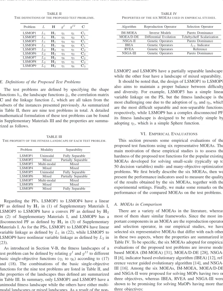
f1 0 0.5 1 1.5 f2 0 0.5 1 1.5 (a) IM-MOEA f1 0 0.5 1 1.5 f2 0 0.5 1 1.5 (b) MOEAD-DE f1 0 0.5 1 1.5 f2 0 0.5 1 1.5 (c) NSGA-II f1 0 1 2 f2 0 0.5 1 1.5 2 2.5 (d) IM-MOEA f1 0 1 2 f2 0 0.5 1 1.5 2 2.5 (e) MOEAD-DE f1 0 1 2 f2 0 0.5 1 1.5 2 2.5 (f) NSGA-II f1 0 0.5 1 1.5 2 f2 0 2 4 (g) IM-MOEA f1 0 0.5 1 1.5 2 f2 0 2 4 (h) MOEAD-DE f1 0 0.5 1 f2 0 1 2 3 4 (i) NSGA-II Fig. 5. The non-dominated solutions obtained by each algorithm on 2-objective LSMOP1, LSMOP6, LSMOP9 in the run associated with the best IGD value.
D. Empirical Results
In the following, we present results obtained by each of the MOEA on the multi-objective and many-objective instances.
1) Results on Multi-Objective Instances: The test prob-lems have 200 or 300 decision variables and two or three objectives, respectively. The statistical results of the IGD values obtained by IM-MOEA, MOEA/D-DE and NSGA-II are summarized in Table VI. In general, none of the three algorithms is able to efficiently solve all instances. To be more specific, IM-MOEA shows the best performance on LSMOP2 and LSMOP6, MOEA/D-DE shows the best performance on LSMOP5, LSMOP7 and LSMOP9, and NSGA-II shows the best performance on 3-objective LSMOP3 and LSMOP8. For further analysis, we have plotted the non-dominated solutions obtained by each algorithm in the best run on three typical problems (LSMOP1, LSMOP6 and LSMOP9) in Fig 5. In the following, we will present some discussions based on the observations made from Fig 5.
LSMOP1 is a relatively simple problem which has a uni-modal and fully separable fitness landscape. Nevertheless, there is still one major difficulty in solving this problem, i.e., the non-uniform variable groups correlated with the two objec-tives. Our results show that, with the non-uniform group size generator presented in (9) and (10), a number of 60 and 145 decision variables are correlated with f1 andf2, respectively.
This means that the decision variables have higher contribution tof2thanf1, thus causing an unbalanced convergence rate of
the two objectives. This phenomenon can be observed from Fig. 5 (a), where the non-dominated solutions obtained by IM-MOEA have significantly better convergence on f1 than on
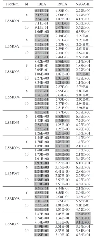
Objective Number 1 2 3 4 5 6 7 8 9 10 Objective Value 0 0.5 1 1.5 2 (a) IBEA Objective Number 1 2 3 4 5 6 7 8 9 10 Objective Value 0 0.5 1 1.5 2 (b) RVEA Objective Number 1 2 3 4 5 6 7 8 9 10 Objective Value 0 0.5 1 1.5 2 (c) NSGA-III Objective Number 1 2 3 4 5 6 7 8 9 10 Objective Value 0 0.5 1 1.5 (d) IBEA Objective Number 1 2 3 4 5 6 7 8 9 10 Objective Value ×105 0 0.5 1 1.5 2 (e) RVEA Objective Number 1 2 3 4 5 6 7 8 9 10 Objective Value 0 500 1000 1500 2000 2500 (f) NSGA-III Objective Number 1 2 3 4 5 6 7 8 9 10 Objective Value 0 0.5 1 1.5 (g) IBEA Objective Number 1 2 3 4 5 6 7 8 9 10 Objective Value 0 5 10 15 20 25 (h) RVEA Objective Number 1 2 3 4 5 6 7 8 9 10 Objective Value 0 20 40 60 (i) NSGA-III Fig. 6. The parallel coordinates of non-dominated solutions obtained by each algorithm on 10-objective LSMOP2, LSMOP3, LSMOP8 in the run associated with the best IGD value.
f2. To confirm this observation, we have calculated the mean
function values of the non-dominated solutions in Fig. 5 (a), and the results indicate that f1 andf2 have a mean value of
0.61 and 1.21, respectively.
LSMOP6 is a partially separable problem which has a complex fitness landscape. The difficulty of this problem is mainly caused by η3 that is correlated with f1. It can be
clearly seen from Fig. 5 (d) to Fig 5 (e) that neither IM-MOEA nor MOEA/D-DE is able to obtain solutions with satisfactory convergence on f1, especially for MOEA/D-DE, which has
converged to a single point on the axis of f2. By averaging
the objective values of the non-dominated solutions in Fig. 5 (b), we can obtain the mean values of f1 and f2, which
are around 1.0×10⁵
(too large to be visible in the figure) and 0, respectively. Such a big difference between the values of the two objectives can cause difficulty for any existing MOEAs, because it leads to a biased convergence towards only one of them due to the highly unbalanced convergence pressures. This phenomenon can also be observed from the results obtained by IM-MOEA in Fig 5 (d). Interestingly, NSGA-II is the only algorithm that has obtained a solution of relatively proper convergence quality on f2. We surmise that
this can be attributed to the fact that the crowding distance based selection in NSGA-II has always preserved the extreme solutions, thus leading to convergence along the directions of the axis.
LSMOP9 has a disconnected PF, although the landscape is not complex. As shown in Fig. 5 (g) to Fig. 5 (i), the solutions obtained by IM-MOEA and MOEA/D-DE have similar con-vergence quality, while IM-MOEA has failed to approximate the second segment of the disconnected PF. Again,
NSGA-II has obtained an extreme solution that has achieved the best convergence on f2, which, however, is the only solution
thus obtained. This phenomenon implies that it is difficult for MOEAs to strike a balance between convergence and diversity on this problem.
Based on the above observations, it can be concluded that the proposed test problems are able to introduce various degrees of difficulties into different objective functions by ap-plying different variable group sizes and correlation matrices. 2) Results on Many-objective Instances: This set of test problems are of 600- or 1000-dimensional and have six or ten objectives, respectively. The statistical results of the IGD values obtained by IBEA, RVEA and NSGA-III are summa-rized in Table VII. Again, none of the three algorithms is able to significantly outperform the others on all these instances. IBEA shows the best performance on LSMOP3 and LSMOP6. To further analyze the results, we have plotted the parallel coordinate of the best non-dominated solution set obtained by each algorithm on LSMOP2, LSMOP3 and LSMOP8 in Fig 6. In the following, we will present some discussions based on the observations from Fig 6.
LSMOP2 is a partially separable problem where the fitness landscape has mixed modality. As shown in Fig. 6 (a) to Fig. 6 (c), the solution sets obtained by the three algorithms show similar convergence quality, while the one obtained by IBEA shows the best distribution, thus leading to the smallest IGD value as shown in Table VII. Since the three algorithms adopt the same reproduction operators (SBX and polynomial mutation), we believe that the advantage of IBEA over the other two algorithms on this problem is due to itsIǫ+indicator
based selection operator.
LSMOP3 has the most difficult multi-modal fitness land-scape among the nine test problems. As shown in Fig. 6 (d), interestingly, IBEA has only obtained one single solution on this problem although its solution set on LSMOP2 shows promising distribution, which implies that it is difficult to always achieve good performance using the same selection strategy on different test problems. However, although the so-lutions sets obtained by RVEA and NSGA-III show relatively better distribution, the convergence quality is quite poor.
LSMOP8 is a problem with both mixed modality and separability. As shown in Fig. 6 (g), again, the solution set obtained by IBEA has achieved promising convergence while the distribution is quite sparse. By contrast, as shown in Fig. 6 (h) and Fig. 6 (i), the solution sets obtained by RVEA and NSGA-III show a denser distribution but worse convergence. Another interesting observation is that RVEA achieves better performance onf1,f2 andf3 than NSGA-III.
To summarize, it turns out that none of the compared algorithms is able to obtain a solution set with both satisfy-ing convergence and distribution performance on the many-objective instances, especially for problems with difficult fitness landscapes such as LSMOP3.
E. Scalability Analysis of Decision Variables
Not many existing test suites for multi- and many-objective optimization have considered the scalability to the number
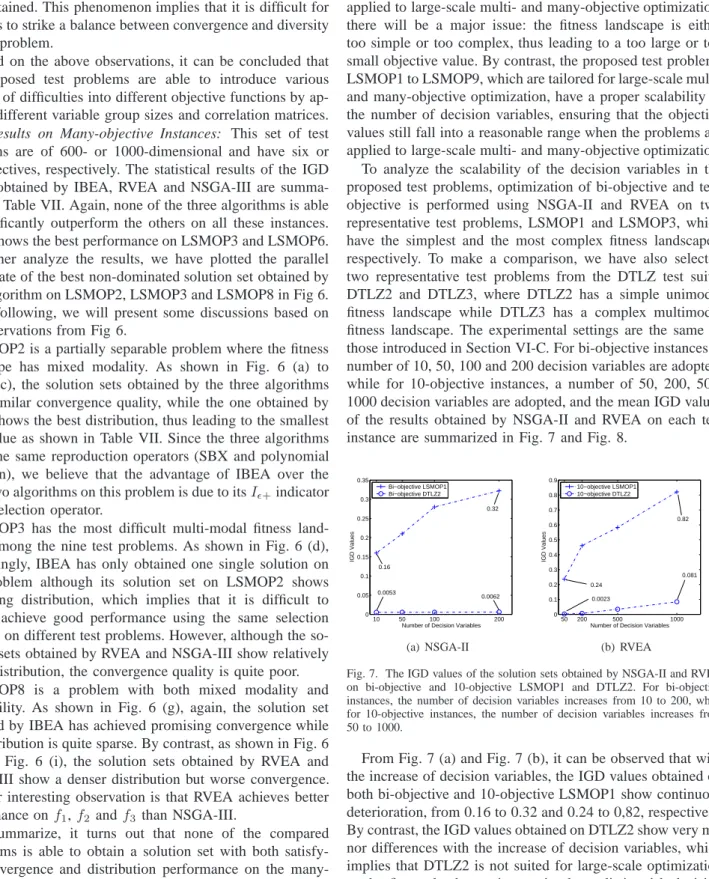
of objectives as they are expected to be only used in small-scale optimization. Therefore, if such test problems are directly applied to large-scale multi- and many-objective optimization, there will be a major issue: the fitness landscape is either too simple or too complex, thus leading to a too large or too small objective value. By contrast, the proposed test problems LSMOP1 to LSMOP9, which are tailored for large-scale multi-and many-objective optimization, have a proper scalability to the number of decision variables, ensuring that the objective values still fall into a reasonable range when the problems are applied to large-scale multi- and many-objective optimization. To analyze the scalability of the decision variables in the proposed test problems, optimization of bi-objective and ten-objective is performed using NSGA-II and RVEA on two representative test problems, LSMOP1 and LSMOP3, which have the simplest and the most complex fitness landscapes, respectively. To make a comparison, we have also selected two representative test problems from the DTLZ test suite, DTLZ2 and DTLZ3, where DTLZ2 has a simple unimodal fitness landscape while DTLZ3 has a complex multimodal fitness landscape. The experimental settings are the same as those introduced in Section VI-C. For bi-objective instances, a number of 10, 50, 100 and 200 decision variables are adopted, while for 10-objective instances, a number of 50, 200, 500, 1000 decision variables are adopted, and the mean IGD values of the results obtained by NSGA-II and RVEA on each test instance are summarized in Fig. 7 and Fig. 8.
10 50 100 200 0 0.05 0.1 0.15 0.2 0.25 0.3 0.35
Number of Decision Variables
IGD Values Bi−objective LSMOP1 Bi−objective DTLZ2 0.32 0.16 0.0053 0.0062 (a) NSGA-II 50 200 500 1000 0 0.1 0.2 0.3 0.4 0.5 0.6 0.7 0.8 0.9
Number of Decision Variables
IGD Values 10−objective LSMOP1 10−objective DTLZ2 0.24 0.0023 0.081 0.82 (b) RVEA
Fig. 7. The IGD values of the solution sets obtained by NSGA-II and RVEA on bi-objective and 10-objective LSMOP1 and DTLZ2. For bi-objective instances, the number of decision variables increases from 10 to 200, while for 10-objective instances, the number of decision variables increases from 50 to 1000.
From Fig. 7 (a) and Fig. 7 (b), it can be observed that with the increase of decision variables, the IGD values obtained on both bi-objective and 10-objective LSMOP1 show continuous deterioration, from 0.16 to 0.32 and 0.24 to 0,82, respectively. By contrast, the IGD values obtained on DTLZ2 show very mi-nor differences with the increase of decision variables, which implies that DTLZ2 is not suited for large-scale optimization as the fitness landscape is too simple to distinguish decision variables of different scales.
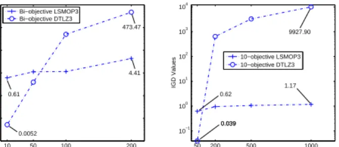
While the landscapes of LSMOP1 and DTLZ2 are simple unimodal, LSMOP3 and DTLZ3 have complex multimodal landscapes. Nevertheless, as evident in Fig. 8 (a) and Fig. 8 (b), with the increase of decision variables, a continuous deterioration of the IGD values is observed, from 0.61 to 4.41
10 50 100 200 10−3 10−2 10−1 100 101 102 103
Number of Decision Variables
IGD Values Bi−objective LSMOP3 Bi−objective DTLZ3 473.47 0.0052 0.61 4.41 (a) NSGA-II 50 200 500 1000 10−1 100 101 102 103 104
Number of Decision Variables
IGD Values 10−objective LSMOP3 10−objective DTLZ3 0.039 0.62 1.17 0.039 9927.90 (b) RVEA
Fig. 8. The IGD values of the solution sets obtained by NSGA-II and RVEA on bi-objective and 10-objective LSMOP3 and DTLZ3. For bi-objective instances, the number of decision variables increases from 10 to 200, while for 10-objective instances, the number of decision variables increases from 50 to 1000.
and 0.62 to 1.17, respectively. By contrast, the IGD values obtained on DTLZ3 show drastic deterioration as the number of decision variables increases from 50 to 1000, which implies that DTLZ3 is not suited for large-scale optimization either, as the fitness landscape is too complex to constraint the objective values within a proper range.
Since LSMOP1 and LSMOP3 are two extreme cases where the fitness landscapes are the simplest one and most complex one, similar observations can also be obtained on the other seven test problems. Such empirical observations indicate that the proposed test problems have proper scalability to the number of decision variables such that the objective values can be constrained within a proper range.
VII. CONCLUSION
This paper proposes a new method for creating test prob-lems for large-scale multi- and many-objective optimization by extending the design principles used in creating multi-objective optimization and large-scale optimization test prob-lems. First, the decision variables are divided into a number of groups of different sizes. Second, the variable groups are correlated with different objective functions, and the correla-tions can be defined easily by means of a correlation matrix. Third, the decision variables have mixed separability.
Nine test problems are instantiated based on the proposed generic principle for designing large-scale multi- and many-objective test problems. Among them, LSMOP1 to LSMOP4 have a linear PF, LSMOP5 to LSMOP8 have a nonlinear PF, and LSMOP9 has a disconnected PF. In addition, the first four test problems (LSMOP1 to LSMOP4) are designed to have linear variable linkages, while the other five test problems (LSMOP5 to LSMOP9) have nonlinear variable linkages. Regarding the fitness landscapes, six widely used basic functions in the single-objective optimization literature have been adopted, three of which are separable and the other three are non-separable. Finally, three types of correlation relationships between the variable groups and the objective functions are proposed, including separable correlation, over-lapped correlation and the full correlation.
To assess the proposed test problems, six representative MOEAs have been tested on the nine instantiations. We have
first tested IM-MOEA, MOEA/D-DE and NSGA-II on bi- and three-objective instances, where the number of decision vari-ables is 200 and 300, respectively. Furthermore, we have tested IBEA, RVEA and NSGA-III on six-objective and ten-objective instances, where the number of decision variables is 600 and 1000, respectively. Our experimental results indicate that the compared algorithms show various strength and weakness on different test problems, and none of them is able to efficiently solve all the proposed problems. This demonstrates that there is a demand for new MOEAs in order to solve such large-scale multi- or many-objective optimization problems with complex separability and correlations, where the new MOEAs should be able to address several basic issues. Firstly, the new MOEAs should be able to detect the non-uniform correlations between decision variables and objectives such that the objectives can be optimized in different orders. Secondly, the new MOEAs should be able to detect the mixed separability of decision variables such that the non-separable subcomponent of the decision vector can be optimized in a divide-and-conquer manner. Thirdly, the new MOEAs should be able to handle the variable linkages on the PSs. Finally, the new MOEAs should also be able to perform efficient and effective search on complex fitness landscapes. As recommended by in [67], the Borg framework can be promising in the design of such new MOEAs, where auto-adaptive techniques is adopted to address some of the above issues, e.g., different selection and reproduction operators can be applied to the search of different fitness landscapes.
It is worth noting that the nine test problems considered in the empirical study is a small set of instantiations created using the proposed design method. Thanks to the extensibility and generic nature of the proposed design principles, more test problems having different separability and correlation properties can be generated.
ACKNOWLEDGEMENTS
This work was supported in part by the Honda Research Institute Europe, the Joint Research Fund for Overseas Chi-nese, Hong Kong and Macao Scholars of the National Natural Science Foundation of China (Grant No. 61428302), and an EPSRC grant (No. EP/M017869/1).
REFERENCES
[1] K. Ikeda, H. Kita, and S. Kobayashi, “Failure of Pareto-based MOEAs: does non-dominated really mean near to optimal?” in Proceedings of the IEEE Congress on Evolutionary Computation, 2001, pp. 957–962. [2] D. Brockhoff, T. Friedrich, N. Hebbinghaus, C. Klein, F. Neumann, and
E. Zitzler, “On the effects of adding objectives to plateau functions,” IEEE Transactions on Evolutionary Computation, vol. 13, no. 3, pp. 591–603, 2009.
[3] O. Sch¨utze, A. Lara, and C. A. C. Coello, “On the influence of the number of objectives on the hardness of a multiobjective optimization problem,” IEEE Transactions on Evolutionary Computation, vol. 15, no. 4, pp. 444–455, 2011.
[4] H. Ishibuchi, N. Tsukamoto, and Y. Nojima, “Evolutionary many-objective optimization: A short review.” in Proceedings of the IEEE Congress on Evolutionary Computation, 2008, pp. 2419–2426. [5] A. Zhou, B.-Y. Qu, H. Li, S.-Z. Zhao, P. N. Suganthan, and Q. Zhang,
“Multiobjective evolutionary algorithms: A survey of the state of the art,” Swarm and Evolutionary Computation, vol. 1, no. 1, pp. 32–49, 2011.