Multi-label classification via multi-target regression on data streams

DOI 10.1007/s10994-016-5613-5

Multi-label classification via multi-target regression on

data streams

Aljaž Osojnik1,2 · Panˇce Panov1 _{· Sašo Džeroski}1,2,3

Received: 26 April 2016 / Accepted: 18 November 2016 / Published online: 30 December 2016 © The Author(s) 2016. This article is published with open access at Springerlink.com

Abstract Multi-label classification (MLC) tasks are encountered more and more frequently in machine learning applications. While MLC methods exist for the classical batch set-ting, only a few methods are available for streaming setting. In this paper, we propose a new methodology for MLC via multi-target regression in a streaming setting. Moreover, we develop a streaming multi-target regressor iSOUP-Tree that uses this approach. We experi-mentally compare two variants of the iSOUP-Tree method (building regression and model trees), as well as ensembles of iSOUP-Trees with state-of-the-art tree and ensemble methods for MLC on data streams. We evaluate these methods on a variety of measures of predictive performance (appropriate for the MLC task). The ensembles of iSOUP-Trees perform signif-icantly better on some of these measures, especially the ones based on label ranking, and are not significantly worse than the competitors on any of the remaining measures. We identify the thresholding problem for the task of MLC on data streams as a key issue that needs to be addressed in order to obtain even better results in terms of predictive performance.

Keywords Multi-label classification·Multi-target regression·Data stream mining

Editors: Nathalie Japkowicz and Stan Matwin.

B

1 _{Jožef Stefan Institute, Jamova Cesta 39, Ljubljana, Slovenia} 2 _{Jožef Stefan International Postgraduate School,}

Jamova Cesta 39, Ljubljana, Slovenia

3 _{Centre of Excellence for Integrated Approaches in Chemistry and Biology of Proteins, Jamova Cesta} 39, Ljubljana, Slovenia

1 Introduction

The task of multi-label classification (MLC) has recently become very prominent in the machine learning research community (Gibaja and Ventura 2015). It can be seen as a gen-eralization of the ubiquitous multi-class classification task, where instead of a single label, each example is associated with multiple labels. This is one of the reasons why multi-label classification is the go-to approach when it comes to automatic annotation of media, such as images, texts or videos, with tags or genres. Most research into multi-label classification has been performed in the batch learning context. However, some effort has also been made to explore multi-label classification in the streaming setting (Qu et al. 2009;Read et al. 2012;

Bifet et al. 2009), following the popularity of big data in the research community, as well as in industry. With an appropriate method, working in the streaming context allows for real-time analysis of large amounts of data, e.g., emails, blogs, RSS feeds, social networks, etc.

Due to the nature of the streaming setting, there are several constraints that need to be considered. A data stream is a potentially infinite sequence of examples, which needs to be analyzed with finite resources, in particular, in finite time and memory. The largest point of divergence from the batch setting is the fact that the underlying concept (that we are trying to learn) can change at any point in time. Therefore, algorithm design is often divided into two parts: (1) learning a stationary concept, and (2) detecting and adapting to its changes. In this paper, we propose a method for multi-label classification in the streaming context that focuses on learning the stationary concept (or more precisely, a set of concepts).

Many algorithms in the literature take the problem transformation approach to multi-label classification, both in the batch and the streaming setting (Read et al. 2008,2011;Tsoumakas and Vlahavas 2007;Fürnkranz et al. 2008). They transform the multi-label classification problem into several problems that can be solved with the off-the-shelf methods, e.g., a transformation into an array of binary classification problems. With this transformation, the label inter-correlations can be lost, and, consequently, the predictive performance can decrease.

In this paper, we take a different perspective and transform the multi-label classification problem into a multi-target regression problem. Multi-target regression is a generalization of single-target regression, used simultaneously predict multiple continuous variables (Struyf and Džeroski 2006;Appice and Džeroski 2007). Many facets of multi-label classification are also present in multi-target regression, e.g., correlation between labels/variables, which motivated us to approach multi-label classification by using multi-target regression methods. To address the label classification task, we have developed a straightforward multi-label classification via multi-target regression methodology, and used it in combination with a streaming multi-target regressor (iSOUP-Tree). The generality is a strong point of this approach, as it allows us to address multiple types of structured output prediction problems, such as multi-label classification and hierarchical multi-label classification, in the streaming setting.

In our initial work on this topic (Osojnik et al. 2015), we performed a set of preliminary experiments with the aim to show that multi-label classification via multi-target regression is a viable approach. We compared our algorithms with basic MLC methods (that give as output a single classifier). We used a very limited number of evaluation measures.

In this paper, we introduce several novel aspects. First, we introduce an adaptive percep-tron in the leaves of the iSOUP-Tree, instead of the simple perceppercep-tron used in the initial work. Furthermore, we introduce an ensemble method (bagging) that uses iSOUP-Trees as base level learners and compare it with the state-of-the-art ensemble method for MLC in a streaming setting. Finally, we significantly extend the experimental methodology and the

experimental questions. In particular, we include a wide range of evaluation measures in the comparison of the different methods and assess whether the overall differences in perfor-mance across all employed methods are statistically significant (by employing appropriate statistical tests).

The structure of the paper is as follows. First, we present the background and related work (Sect.2). Next, we present the approach of multi-label classification via multi-target regres-sion on data streams (Sect.3) and our iSOUP-Tree method for MTR on data streams (Sect.4). Furthermore, we present the research questions and the experimental design (Sect.5). We then present and discuss the results (Sect.6). Finally, we outline our conclusions and some directions for further work (Sect.7).

2 Background and related work

In this section, we review the state-of-the art in multi-label classification, both in the batch and the streaming context. In addition, we present the background of the multi-target regression task, which we use as a foundation for defining the multi-label classification via multi target regression approach.

2.1 Multi-label classification

Generalizing multi-class classification, where only one of the possible labels needs to be predicted,multi-label classificationrequires a model to predict a combination (subset) of the possible labels. Formally, this means that for each data instancexfrom an input spaceXa model needs to provide a predictionyˆfrom an output spaceY, which is a powerset of the labelsetL, i.e.,Y =2L. This is in contrast to the multi-class classification task, where the output space is simply the labelsetY =L. We denote the real labels of an instancexbyy, and a prediction made by a model forxbyyˆ(x)(or simplyy).ˆ

In the batch setting, the problem transformation approach is commonly used to tackle the task of multi-label classification. Problem transformation methods are usually used as basic methods to compare to, and are used in a combination with off-the-shelf base algorithms. The most common approach, calledbinary relevance (BR), transforms a multi-label task into several binary classification tasks, one for each of the possible labels (Read et al. 2011). Binary relevance models have been often overlooked due to their inability to account for label correlations, though some BR methods are capable of modeling label correlations during classification.

Another common problem transformation approach is thelabel combination orlabel powerset(LC) method, where each subset of the labelset is considered as an atomic label for a multi-class classification problem (Read et al. 2008;Tsoumakas and Vlahavas 2007). If we start with a multi-label classification task with a labelset ofL, we transform this into a multi-class classification with a lablesetL=2L.

The third most common problem transformation approach ispairwise classification, where we have a binary model for each possible pair of labels (Fürnkranz et al. 2008). This method performs well in some contexts. For larger problems the method becomes intractable because of model complexity.

In addition to problem transformation methods, there are also adaptations of the well known algorithms that handle the task of multi-label classification directly. Examples of such algorithms are the adaptation of the decision tree learning algorithm for MLC (Vens et al. 2008), support-vector machines for MLC (Gonçalves et al. 2013), k-nearest neighbours

for MLC (Zhang and Zhou 2005), instance based learning for MLC (Cheng and Hüllermeier 2009), and others.

2.2 Multi-label classification on data streams

Many of the problem transformation methods for multi-label classification have also been used in the streaming context. Unlike the batch context, where a fixed and complete dataset is given as input to a learning algorithm, the streaming context presents several limitations that the stream learning algorithm must take into account.Bifet and Gavaldà(2009) define the most relevant ones as follows: (1) the examples arrive sequentially; (2) there can potentially be infinitely many examples; (3) the distribution of examples need not be stationary; and (4) after an example is processed it is discarded or archived. The fact that the distribution of examples is not presumed to be stationary means that algorithms should be able to detect and adapt to changes in the distribution (concept drift).

The first approach to MLC in data streams was a batch-incremental method that trains stacked BR classifiers (Qu et al. 2009). Some methods for multi-class classification, such as Hoeffding Trees (HT) (Domingos and Hulten 2000), have also been adapted to the multi-label classification task (Read et al. 2012). Hoeffding trees are incremental anytime decision trees for learning from data streams that use the notion that a small sample is usually sufficient for choosing an optimal splitting attribute, i.e., the use of the Hoeffding bound.Read et al.(2012) proposed the use of multi-label Hoeffding trees with pruned sets (PS) at the leaves(HTPS), as well as using them in combination with the ADWIN bagging (Bifet et al. 2009) ensemble method, which implicitly addresses the problems of change detection and adaptation.Bifet et al.(2010) introduced the Java-based Massive Online Analysis (MOA)1framework, which also allows for the analysis of concept drift (Bifet and Gavaldà 2009) and has become one of the main software frameworks for data stream mining.

Recently,Spyromitros-Xioufis(2011) introduced a parameterized windowing technique for dealing with concept drift in multi-label data in a data stream context. Next,Shi et al.

(2014a) proposed an efficient and effective method to detect concept drift based on label grouping and entropy for multi-label data, where the labels are grouped by using clustering and association rules. This allowed for an effective detection of concept drift which takes into account label dependence. Finally,Shi et al.(2014b) proposed an efficient class incremental learning algorithm, which dynamically recognizes some new frequent label combinations.

2.3 Multi-target regression

In the same way as multi-label classification generalizes regular (single target) classification, multi-target regression task is an extension of single-target regression. Multi-target regression (MTR) is the task of predicting multiple numeric variables simultaneously. Formally, the task is to make a predictionyˆfromRn, wherenis the number of targets for a given instancex

from an input spaceX.

As in multi-label classification, there is a common problem transformation method that transforms the multi-target regression problem into multiple single-target regression prob-lems. In this case, we consider each numeric target separately and train a single-target regressor for each of them. However, thislocalapproach suffers from similar problems as the problem transformation approaches to multi-label classification: The single target mod-els do not consider the inter-correlations of the target variables. The task of simultaneous prediction of all target variables at the same time (theglobalapproach) has been considered 1_{URL:http://moa.cms.waikato.ac.nz/, accessed on 2016/04/23.}

in the batch setting byStruyf and Džeroski(2006). In addition,Appice and Džeroski(2007) proposed an algorithm for stepwise induction of multi-target model trees. Finally,Xioufis et al.(2016) introduced two new methods for multi-target regression (called Stacked Single-Target and Ensemble of Regressor Chains) by adapting multi-label classification methods. The methods treat the other prediction targets as additional input variables and exploit the target dependencies in order to improve the accuracy of their predictions.

In the streaming context, some work has been done on multi-target regression.

Ikonomovska et al.(2011b) introduced an instance-incremental streaming tree-based single-target regressor (FIMT-DD) that utilized the Hoeffding bound. This work was later extended to the multi-target regression setting (Ikonomovska et al. 2011a) (FIMT-MT). There has been a theoretical debate on whether the use of the Hoeffding bound is appropriate (Rutkowski et al. 2013), but, a recent study byIkonomovska et al.(2015) has shown that, in practice, the use of the Hoeffding bound produces good results. However, the drawback of these algorithms is that they ignore nominal input attributes. Recently,Duarte and Gama(2015) implemented a rule-based learning approach for multi-target regression (AMRules), while

Shaker and Hüllermeier(2012) introduced an instance-based system for classification and regression (IBLStreams), which can be used for multi-target regression.

3 Multi-label classification via multi-target regression

The problem transformation methods (see Sect.2.1) generally transform a multi-lablel clas-sification task into one, or several, binary or multi-class clasclas-sification tasks. In this paper, we take a different approach and transform a classification task into a regression task. The simplest example of a transformation of this type is to transform a binary classification task into a regression task. For example, if we have a binary target with labelsyesandno, we would consider a numeric target to which we would assign a numeric value of 0 if the binary label isnoand 1 if the binary label isyes.

In the same way, we can approach the multi-class classification task. Specifically, if the multi-class target variable is ordinal, i.e., the class labels have a meaningful ordering, we can assign the numeric values from 0 ton−1 to each of the correspondingnlabels. This makes sense, since if the labels are ordered, a misclassification of a label into a “nearby” label is better than a misclassification into a “distant” label. However, if the variable is not ordinal this makes less sense, as any given label is not in a strict relationship with other labels.

In that case, an approach similar to that introduced byFrank et al.(1998) to address multi-class classification using regression can be used. In their case, they produced several versions of the observed data, one version per class in the multi-class classification task. For each class, its version of the data featured a derived binary classification target, which corresponded to the presence of the class. Consequently, for each class a model tree regressor was learned. For a given example, the prediction of each of the trees was calculated, after which the example was classified into the class with the highest corresponding (numeric) tree prediction. This approach produces one regressor per class, however, with the use of methods for multi-target regression, this can be reduced to one (multi-target) regressor for all of the classes.

To address the label classification task using regression, we transform it into a multi-target regression task (see Fig.1). This procedure is performed in two steps: first, we take the viewpoint that the multi-label classification target is composed of several binary classification variables, just as in the BR method. However, instead of training one classifier for each of

R T M C L M

Target space _{y⊆ L{λ1, . . . , λn} −−−−−−−−−−→}transformation _y∈Rn

Instance _{y={λ1, λ3, λ4} −−−−−−−−−−→}transformation _{y= (1,0,1,1, . . .)} Fig. 1 Transformation of a MLC problem to a MTR problem. Only the target space is transformed. Applied before learning a multi-target regressor

C L M R T M

Target space _yˆ∈Rn thresholding

−−−−−−−−→ ˆy⊆ L Instance _{yˆ= (0.98,0.21,0.59,0.88, . . .)} thresholding

−−−−−−−−→ yˆ={λ1, λ3, λ4}

Fig. 2 From MTR to MLC. Transforming a multi-target regression prediction into a multi-label classification one

the binary variables, we further transform the values of the binary variable into numbers. A numeric target corresponding to a given label has a value 1 if the label is present in a given instance, and a value 0 if the label is not present.

For example, if we have a multi-label classification task with target labels L =

{red,blue,green}, we transform it into a multi-target regression task with three numeric target variablesyred,yblue,ygreen ∈R. If an instance is labeled with red and green, but not blue, the corresponding numeric targets will have valuesyred=1,yblue=0, andygreen=1. Since we are using a regressor, it is possible that a prediction for a given instance will not result in a value of exactly 0 or 1 for each of the targets. For this purpose, we use thresholding to transform back a multi-target regression prediction into a multi-label one (see Fig.2). Namely, we construct the multi-label prediction in such a way that it contains labels with numeric values over a certain threshold, i.e., in our case, the labels selected are those with a numeric value over the threshold ofτ =0.5. It is clear, however, that a different choice of threshold leads to different predictions.

In the batch setting, thresholding can be performed in the pre- and postprocessing phases. However, in the streaming setting it needs to be done in real time. Specifically, the process of thresholding occurs at two times. The first thresholding occurs when the multi-target regressor has produced a target prediction, which must then be converted into a multi-label prediction. The second thresholding occurs when we are updating the regressor, i.e., when the regressor is learning. Most streaming regressors are heavily dependent on the values of the target variables in the learning process, so the instances must be converted into the numeric representation that the multi-target regressor can utilize.

The problem of thresholding is not only problematic in the MLC via MTR setting, but also when considering the MLC task with other approaches. In general, MLC models pro-duce results which are interpreted as probability estimations for each of the labels, thus the threhsolding problem is a fundamental part of multi-label classification.

4 The iSOUP-Tree method

To utilize the MLC via MTR approach, we have reimplemented the FIMT and FIMT-MT algorithms (Ikonomovska et al. 2011a) in the MOA framework to facilitate usability and visibility, as the original implementation was a standalone extension of the C-based VFML library (Hulten and Domingos 2003) and was not available as part of a larger data stream

mining framework. We have also significantly extended the algorithm to consider nominal attributes in the input space when considering splitting decisions. This allows us to use the algorithm on a wider selection of datasets, some of which are considered herein.

In this paper, we combined the multi-label classification via multi-target regression methodology, proposed in the previous section, with the extended version of FIMT-MT, reim-plemented in MOA. We named this method the incremental Structured OUtput Prediction Tree (iSOUP-Tree), since it is capable of addressing multiple structured output prediction tasks, i.e., multi-label classification and multi-target regression.

Ikonomovska et al.(2011b) have considered the performance of FIMT-DD when a simple predictive model is placed in each of the leaves, i.e., in this case a single linear unit (a perceptron).Model treesproduce the predictions as a linear combination of input attribute values, i.e., yˆ(x) = m_i=1xiwi+b, wheremis the number of input attributes andwi,b

are the perceptron weights, respectively. In contrast, inregression treesthe prediction in a given leaf for an instancexis made for each of the targets as the average value of the recorded target values,yˆ(x) = _|S|1 _y∈Sy, whereS is the set of observed examples in a given leaf. It was shown that using model trees yields better performance. However, this was only experimentally confirmed for regression tasks. In regression the targets generally exhibit larger variation than in classification tasks.

Our initial research showed that the use of a simple perceptron in the leaves provides very bad experimental results in the MLC via MTR setting (Osojnik et al. 2015). To correct this, we have replaced the perceptron with an adaptive perceptron, as done byDuarte and Gama

(2014). This adaptive perceptron combines the predictions of the perceptron and the mean target predictor.

4.1 Adaptive perceptron

In the original implementation of FIMT byIkonomovska et al.(2011b), the perceptron was always used to make the prediction. However, the adaptive model in a given tree leaf records the errors of the perceptron and compares them to the errors of the mean target predictor, which predicts the value of the target by computing the average value of the target over the examples observed in the leaf. In essence, each leaf has two predictors, the perceptron and the target mean predictor. The prediction of the predictor with the lower error (at a given point in time) is then used as the output prediction.

To monitor the errors, we use the faded mean absolute error which is calculated as fMAE_predictor(m)= m i=10.95m−i| ˆyi−yi| m i=10.95m−i ,

wheremis the number of observed examples in a leaf,yˆiandyiare the predicted and real

value for theith example, respectively, andpredictor∈ {perceptron,targetMean}. The faded error is, in essence, weighted towards more recent examples. Intuitively, the numerator of the above fraction is the faded sum of absolute errors, while the denominator is the faded count of examples. For example, the most recent (mth) example contributes with a weight of 1, the previous example with weight 0.95, and the first example with weight 0.95m−1. This places a large emphasis on more recent examples and generally benefits the perceptron, as we expect its errors to decrease as it learns the weight vector.

However, we have to be careful when considering a classification task through the lens of regression. In classification, the actual target variables can only take values of 0 and 1. If we use a linear model such as a perceptron (or the adaptive perceptron described above) to predict one of the targets, we have no guarantee that the predicted value will land in the[0,1]interval.

A regression tree’s prediction will produce a prediction which is calculated as an average of zeroes and ones, which will always land in this interval. Additionally, the perceptrons in the leaves are trained in real-time according to theWidrow-Hoff rule, which consumes a non-negligible amount of time, which can be a constraint in the data stream mining setting. Hence, we are motivated to consider the use of both multi-target regression trees as well as target model trees when addressing the task of label classification via multi-target regression. We denote the regression tree variation of iSOUP-Tree asiSOUP-RTand the model tree variant asiSOUP-MT.

4.2 Ensembles

In addition to observing and evaluating a single regression or model tree, we also consider ensembles of iSOUP-Trees. We use theonline baggingapproach introduced byOza(2005), which naturally extends the approach for bagging from the batch setting. In essence, each of the incoming examples is assigned to each of the members of the ensemble a different number of times, i.e., for each example-ensemble member pair we sample the Poisson distribution with parameterλ= 1 to determine the number of repetitions of the given example to the given ensemble member. The theoretical motivation behind this methodology is concisely explained in the original paper. We denote the bagging of iSOUP regression treesEBRT2

and the bagging of model trees asEBM T.

Ensembles can also be used to address the problem of drift detection and adaptation. ADWIN bagging (Bifet et al. 2009) is an extension of the above ensemble methodology, which monitors the performance of the ensemble members and discards under-performing models, and replaces them with new empty models, which are learned anew. However, we specifically avoid the use of ADWIN bagging, as we wish to address the problem of change detection and adaptation even in the single-tree scenario.

5 Experimental design

In this section, we first present the experimental questions that we want to answer. Next, we describe the datasets and algorithms used in the experiments. Furthermore, we discuss the evaluation measures used in the experiments. Finally, we conclude with a description of the employed experimental methodology.

5.1 Experimental questions

Our experimental design is constructed in such a way to address several lines of inquiry. First, we investigate whether if the use of model trees with the adaptive perceptron improves predic-tive performance over regression trees. Namely, we have shown a previous study that using model trees with regular preceptrons produces considerably worse results than regression trees (Osojnik et al. 2015).

Second, we comparatively evaluate the performance of the introduced single tree methods to the Hoeffding tree with pruned sets (HTPS) (Read et al. 2012). The latter is a direct (single)

tree-based competitor, which does not utilize the MLC via MTR methodology. This allows further investigates the viability of the proposed methodology for MLC.

2_{E denotes that the method learns an ensemble, while the B determines that bagging is used to achieve} variation among the base models.

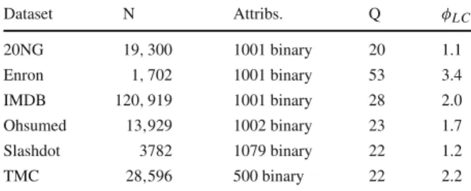
Table 1 Datasets used in the

experiments Dataset N Attribs. Q φLC

20NG 19,300 1001 binary 20 1.1 Enron 1,702 1001 binary 53 3.4 IMDB 120,919 1001 binary 28 2.0 Ohsumed 13,929 1002 binary 23 1.7 Slashdot 3782 1079 binary 22 1.2 TMC 28,596 500 binary 22 2.2 Nnumber of instances,Q

number of labels,φLCaverage

number of labels per instance

Furthermore, we compare all of the methods, including ensemble-based approaches, to determine how the methods rank both in terms of performance and efficiency, as well as to observe the effect of using ensembles of the base learners.

Finally, we observe the methods’ efficiency to determine what, if any, trade-offs in terms of performance versus resource use are made when using the different methods.

5.2 Datasets

In our experiments, we use a subset of the datasets listed inRead et al.(2012, Tab. 3) (see Table1). Here, we briefly describe the dataset domains:

– The20 newsgroupsis a dataset comprised of a collection of articles from 20 newsgroups. – TheEnrondataset (Read 2008) is a collection of labelled emails, which, though small by data stream standards, exhibits some data stream properties, such as time-order and evolution over time.

– TheIMDBdataset is constructed from text summaries of movie plots from the Internet Movie Database and is labelled with the relevant genres.

– TheOhsumeddataset was constructed from a collection of peer-reviewed medical articles and labelled with the appropriate disease categories.

– The datasetSlashdotwas collected from thehttp://slashdot.orgweb page and consists of article blurbs labelled with subject categories.

– TheTMCdataset was used in the SIAM 2007 Text Mining Competition and consists of human generated aviation safety reports, labelled with the problems being described (we are using the version of the dataset specified inTsoumakas and Vlahavas(2007)). With the exception of the TMC dataset, all datasets are available at the MEKA project page.3 The TMC dataset is available at the Mulan data repository.4

5.3 Algorithms

To address our experimental questions, we performed experiments using our implementations of the algorithms for learning multi-target model trees (iSOUP-MTorMTfor brevity) and multi-target regression trees (iSOUP-RTorRT). In addition, we also use ensemble methods, specifically, online bagging for iSOUP-RT (EBRT) and iSOUP-MT (EBMT). The testing for

splits occurs at intervals of 200 observed examples, with the Hoeffding bound confidence level (theδparameter) set to 0.0000001.

3_{https://sourceforge.net/projects/meka/files/Datasets/, accessed on 2016/03/11.} 4_{http://mulan.sourceforge.net/datasets-mlc.html, accessed on 2015/05/25.}

The MLC setting has not received as much attention in the streaming setting as it has in the batch setting, therefore, there aren’t as many competing algorithms as there would be in the batch setting. We chose the updated implementation5_{ofRead et al.(2012), which learns}

Hoeffding trees with pruned sets (HTPS), as well as ADWIN bagging for Hoeffding trees

with pruned sets (EAH TPS).6The parameters of these methods were set as suggested by the

authors.

5.4 Evaluation measures

In the evaluation, we use a set of measures used in recent surveys and experimental compar-isons of different multi-label algorithms in the batch setting (Madjarov et al. 2012;Gibaja and Ventura 2015). The evaluation measures are grouped into four segments: example-based measures (accuracy, F1, Hamming score), label-based measures (macro precision, macro recall, macro F1, micro precision, micro recall, micro F1), ranking-based measures (average precision, ranking loss, logarithmic loss), and efficiency measures (memory consumption and time). This yields a total of 12 measures of predictive performance and 2 measures of efficiency.

From the above, it is clear that in the MLC setting performance along a wide variety of measures can be investigated. Example-based measures evaluate the quality of classification on a per-example basis, i.e., how good is the classification over different examples, while label-based measures evaluate the quality of the classification on a per-label basis, i.e., how good is the classification over different labels. Ranking-based measures evaluate the classi-fication based on the ordering of the labels according to their presence, e.g., a classiclassi-fication is evaluated more positively if the present labels are ranked higher, often without regard for the thresholding procedure.

In particular, example-based and label-based measures are calculated based on the com-parison of the predicted labels with the ground truth labels. On one hand, example-based measures depend on the average difference of the actual and predicted sets of labels over the complete set of data examples from the evaluation set. On the other hand, label-based measures assess the performance for each label separately and than average the performance over all labels. The models produced by algorithms used in this study give as prediction numerical values for each of the labels. The label is predicted as present if the numerical value exceeds a predefined thresholdτ(in our case we set the value to 0.5). This means that both example-based and label-based measures are directly dependent on the choice of the parameterτ. Ranking-based evaluation measures, however, compare the predicted ranking of the labels with the ground truth ranking and do not necessarily depend on the choice of the threshold parameter. The full definitions of the observed measures can be found in “Appendix”.

To measure the efficiency of the observed methods we consider the running time, measured in seconds, with a resolution of one hundredth of a second, and the total amount of memory consumed in MB. The time measurements exclusively measure the learning time and the time used to make predictions, excluding other processes such as loading of examples from the file system and the calculation of evaluation measures. In the case of time and memory usage, we desire low values.

5_{The methods are implemented as part of the MEKA and MOA frameworks.} 6_{As before, E denotes the use of an ensemble, while the A stands for ADWIN bagging.}

Each evaluation measure presents and choosing which to optimize in a real-world scenario is dependent on the desired outcomes. The performance of competing methods is, therefore, evaluated separately using each measure. However, note that ranking-based measures are of special importance, as they do not require threhsholding, while precision and recall can be traded off by selecting a different threshold.

5.5 Experimental setup

For all of our experiments we are using thepredictive sequential(prequential) evaluation methodology for data streams (Gama 2010). This means that for each example, first a pre-diction is made and collected, and second, the example is used to update the model. Once predictions for each of the examples are collected, the evaluation measures are calculated on all of the predictions. Using prequential evaluation ensures that the model has as much information as possible to make the prediction for each example. However, the prequential evaluation methodology is more optimistic than the other commonly usedholdoutevaluation approach, where a window of examples is constructed and the entire window is first used to make predictions and then to update the model.

Unlike the holdout methodology, the prequential evaluation methodology allows the model to use all of the information available at a given point to make a prediction, as all of the preceding examples are used to update the model prior to making a prediction. While in real-world applications either evaluation methodology could be the correct choice, in this paper, we chose to observe the performance of the methods in the most optimistic scenario. More specifically, we constructed the following experimental setup to answer the proposed experimental questions. This experimental setup is designed to be a streaming analog of the commonly used batch MLC experimental setup, e.g., used byMadjarov et al.(2012) andRead et al.(2009), and is very similar to the setup used byRead et al.(2012) in the streaming setting. For each of the datasets, we used the prequential methodology to calculate the predictions of all of the models on all of the instances in the dataset. The predictions are then thresholded to calculate the label-based and example-based measures on the entire dataset, while the ranking measures are calculated using the unthresholded predictions. The recorded measurements are therefore calculated using the obtained predictions over the entire dataset. Additionally, we measured the time and memory used to learn and make predictions.

To assess whether the overall differences in performance across all employed methods are statistically significant for a given evaluation measure, we employed the corrected Friedman test (Friedman 1940) and the post-hoc Nemenyi test (Nemenyi 1963) as recommended by

Demšar(2006). The results of the statistical test are represented in the form of average rank diagrams for each evaluation measure. These form the basis on which we build the answers to our experimental questions and form our conclusions. When comparing only two methods, i.e., in the case of the comparison of regression and model trees as well as the comparison of different single-tree methods, we also refer to the results on the individual datasets.

6 Results and discussion

The results of the evaluation are grouped by the type of evaluation measure for ease of discussion. Within each group of evaluation measures, we discuss their relevance to our experimental questions. Afterwards, we wrap up with a discussion of the implication of the complete set of results to the experimental questions.

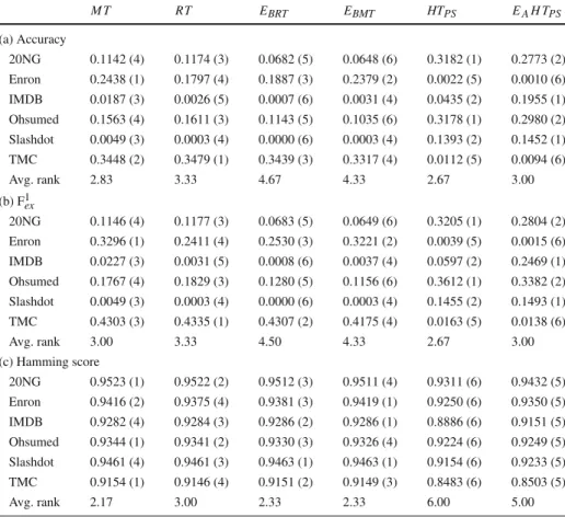
Table 2 Predictive performance results: example-based measures M T RT EBRT EBMT HTPS EAH TPS (a) Accuracy 20NG 0.1142 (4) 0.1174 (3) 0.0682 (5) 0.0648 (6) 0.3182 (1) 0.2773 (2) Enron 0.2438 (1) 0.1797 (4) 0.1887 (3) 0.2379 (2) 0.0022 (5) 0.0010 (6) IMDB 0.0187 (3) 0.0026 (5) 0.0007 (6) 0.0031 (4) 0.0435 (2) 0.1955 (1) Ohsumed 0.1563 (4) 0.1611 (3) 0.1143 (5) 0.1035 (6) 0.3178 (1) 0.2980 (2) Slashdot 0.0049 (3) 0.0003 (4) 0.0000 (6) 0.0003 (4) 0.1393 (2) 0.1452 (1) TMC 0.3448 (2) 0.3479 (1) 0.3439 (3) 0.3317 (4) 0.0112 (5) 0.0094 (6) Avg. rank 2.83 3.33 4.67 4.33 2.67 3.00 (b) F1ex 20NG 0.1146 (4) 0.1177 (3) 0.0683 (5) 0.0649 (6) 0.3205 (1) 0.2804 (2) Enron 0.3296 (1) 0.2411 (4) 0.2530 (3) 0.3221 (2) 0.0039 (5) 0.0015 (6) IMDB 0.0227 (3) 0.0031 (5) 0.0008 (6) 0.0037 (4) 0.0597 (2) 0.2469 (1) Ohsumed 0.1767 (4) 0.1829 (3) 0.1280 (5) 0.1156 (6) 0.3612 (1) 0.3382 (2) Slashdot 0.0049 (3) 0.0003 (4) 0.0000 (6) 0.0003 (4) 0.1455 (2) 0.1493 (1) TMC 0.4303 (3) 0.4335 (1) 0.4307 (2) 0.4175 (4) 0.0163 (5) 0.0138 (6) Avg. rank 3.00 3.33 4.50 4.33 2.67 3.00 (c) Hamming score 20NG 0.9523 (1) 0.9522 (2) 0.9512 (3) 0.9511 (4) 0.9311 (6) 0.9432 (5) Enron 0.9416 (2) 0.9375 (4) 0.9381 (3) 0.9419 (1) 0.9250 (6) 0.9350 (5) IMDB 0.9282 (4) 0.9284 (3) 0.9286 (2) 0.9286 (1) 0.8886 (6) 0.9151 (5) Ohsumed 0.9344 (1) 0.9341 (2) 0.9330 (3) 0.9326 (4) 0.9224 (6) 0.9249 (5) Slashdot 0.9461 (4) 0.9461 (3) 0.9463 (1) 0.9463 (1) 0.9154 (6) 0.9233 (5) TMC 0.9154 (1) 0.9146 (4) 0.9151 (2) 0.9149 (3) 0.8483 (6) 0.8503 (5) Avg. rank 2.17 3.00 2.33 2.33 6.00 5.00

Each table contains the values of the measure (and the rank) of each method on each dataset

6.1 Results on the example-based measures

The values and rankings on the example-based measures (accuracy, F1

exand Hamming score)

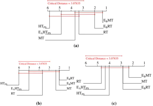
are presented in Table2. The results of the Friedman-Nemenyi significance tests are presented in Fig.3in the form of average rank diagrams.

With regards to the comparison of iSOUP model and regression trees, the average rank of model trees is higher than the average rank of regression trees in all example-based measures, even though the difference is not statistically significant. The results on individual datasets in terms of the Hamming score are nearly identical, while model trees are slightly better on the accuracy and F1_exmeasures. Even when regression trees beat model trees on a particular dataset, the difference in performance is much smaller than when model trees perform better. The results of the comparison between the single-tree methods on the example-based evaluation measures are not entirely clear-cut. For both accuracy and F1_ex, the average rank of theHTPS method is higher than the average ranks of model and regression trees, but

the difference is not statistically significant. TheHTPSmethod has poorer performance on

the Enron and TMC datasets, where regression and model trees both outperformHTPS.

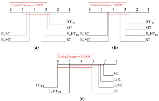
6 5 4 3 2 1 HTPS MT EAHTPS RT EBMT EBRT Critical Distance = 3.07835 (a) 6 5 4 3 2 1 HTPS MT EAHTPS RT EBMT EBRT Critical Distance = 3.07835 (b) 6 5 4 3 2 1 MT E_BRT E_BMT RT EAHTPS HT_PS Critical Distance = 3.07835 (c)

Fig. 3 Average rank diagrams for the example-based measures.aAccuracy,bF1_ex,cHamming score and regression trees are much higher than the rank of theHTPSmethod. The difference in

performance between model trees and theHTPSmethod is in this case statistically significant.

When examining the performance of the learning methods in terms of the accuracy and F1_exin detail (per dataset), we again observe very mixed results. It is noticeable that, on some datasets, a group of methods has orders of magnitude better results than the other methods, i.e.,HTPS andEAH TPS on the Slashdot dataset,M T,RT,EBMTandEBRTon the Enron

dataset, andEAH TPSon the IMDB dataset. We found no statistically significant differences

in performance for both the accuracy measure (Fig.3a) as well as the F1_exmeasure (Fig.3b). On the other hand, the results in terms of the Hamming score are much clearer.M T,RT, EBMTandEBRThave higher average rank thanHTPSandEAHTPS. However, according to

the Friedman-Nemenyi post-hoc test, onlyHTPSis significantly worse thanM T,EBRTand

EBMT(Fig.3c).

6.2 Results on the label-based measures

The performance measure values and rankings for the label-based measures (Precisionmacro,

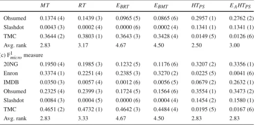
Recallmacro, F1macro, Precisionmicro, Recallmicroand F1micro) are presented in Tables3and4.

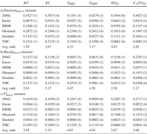
The results of the Friedman-Nemenyi post-hoc significance tests are presented in Fig.4. On all macro label-based evaluation measures, model trees get results better than or about equal to the results of regression trees. While regression trees do outperform model trees on some datasets, e.g., for all of the macro measures on the Ohsumed dataset, the differences in these cases are relatively small, while when the model trees outperform regression trees, e.g., for all macro measures on the IMDB dataset, the differences are considerably larger. For all three measures, the difference in average ranks of the methods is not statistically significant. The results on the micro measures are similar. Model trees have higher average rank than regression trees in terms of Precisionmicro, though the differences are not statistically

Table 3 Predictive performance results: label-based measures (macro)

M T RT EBRT EBMT HTPS EAH TPS

(a) Precisionmacromeasure

20NG 0.5527 (1) 0.3873 (4) 0.3351 (5) 0.4279 (3) 0.1944 (6) 0.4427 (2) Enron 0.0679 (1) 0.0341 (6) 0.0427 (5) 0.0588 (3) 0.0643 (2) 0.0474 (4) IMDB 0.2306 (2) 0.1452 (3) 0.0576 (5) 0.2824 (1) 0.0392 (6) 0.1157 (4) Ohsumed 0.2872 (2) 0.2946 (1) 0.2788 (3) 0.2612 (4) 0.1653 (6) 0.1907 (5) Slashdot 0.1347 (2) 0.0152 (5) 0.0000 (6) 0.0227 (4) 0.1311 (3) 0.1842 (1) TMC 0.3321 (1) 0.3135 (3) 0.3185 (2) 0.2380 (4) 0.0081 (6) 0.0083 (5) Avg. rank 1.50 3.67 4.33 3.17 4.83 3.50

(b) Recallmacromeasure

20NG 0.1127 (4) 0.1156 (3) 0.0667 (5) 0.0635 (6) 0.3156 (1) 0.2787 (2) Enron 0.0319 (1) 0.0193 (4) 0.0205 (3) 0.0299 (2) 0.0096 (5) 0.0019 (6) IMDB 0.0060 (3) 0.0012 (4) 0.0002 (6) 0.0010 (5) 0.0411 (2) 0.0557 (1) Ohsumed 0.0840 (4) 0.0884 (3) 0.0495 (5) 0.0406 (6) 0.1623 (1) 0.1433 (2) Slashdot 0.0021 (3) 0.0001 (4) 0.0000 (6) 0.0001 (4) 0.0861 (1) 0.0586 (2) TMC 0.1237 (2) 0.1332 (1) 0.1070 (3) 0.0981 (4) 0.0413 (5) 0.0388 (6) Avg. rank 2.83 3.17 4.67 4.50 2.50 3.17 (c) F1_macromeasure 20NG 0.1619 (4) 0.1630 (3) 0.1047 (5) 0.0999 (6) 0.2287 (2) 0.2717 (1) Enron 0.0364 (1) 0.0199 (4) 0.0217 (3) 0.0340 (2) 0.0127 (5) 0.0032 (6) IMDB 0.0113 (3) 0.0023 (4) 0.0004 (6) 0.0019 (5) 0.0239 (2) 0.0540 (1) Ohsumed 0.1210 (4) 0.1269 (3) 0.0745 (5) 0.0617 (6) 0.1586 (1) 0.1523 (2) Slashdot 0.0041 (3) 0.0002 (5) 0.0000 (6) 0.0002 (4) 0.0627 (1) 0.0487 (2) TMC 0.1503 (2) 0.1605 (1) 0.1228 (3) 0.1110 (4) 0.0064 (5) 0.0041 (6) Avg. rank 2.83 3.33 4.67 4.50 2.67 3.00

Each table contains the values of the measure (and the rank) of each method on each dataset

Table 4 Predictive performance results: label-based measures (micro)

M T RT EBRT EBMT HTPS EAHTPS

(a) Precisionmicromeasure

20NG 0.7408 (3) 0.7189 (4) 0.8227 (2) 0.8270 (1) 0.3253 (6) 0.4218 (5) Enron 0.6108 (2) 0.5363 (4) 0.5539 (3) 0.6249 (1) 0.0664 (6) 0.0863 (5) IMDB 0.4411 (3) 0.3746 (4) 0.5242 (2) 0.5864 (1) 0.0844 (6) 0.3461 (5) Ohsumed 0.7561 (3) 0.7216 (4) 0.8086 (2) 0.8189 (1) 0.4453 (6) 0.4677 (5) Slashdot 0.3220 (1) 0.0556 (5) 0.0000 (6) 0.2500 (2) 0.1587 (4) 0.1923 (3) TMC 0.6427 (2) 0.6263 (4) 0.6394 (3) 0.6481 (1) 0.0280 (5) 0.0248 (6) Avg. rank 2.33 4.17 3.00 1.17 5.50 4.83

(b) Recallmicromeasure

20NG 0.1123 (4) 0.1151 (3) 0.0666 (5) 0.0633 (6) 0.3161 (1) 0.2786 (2) Enron 0.2330 (1) 0.1424 (4) 0.1520 (3) 0.2214 (2) 0.0136 (5) 0.0021 (6) IMDB 0.0182 (3) 0.0029 (4) 0.0006 (6) 0.0028 (5) 0.0568 (2) 0.2123 (1)

Table 4 continued M T RT EBRT EBMT HTPS EAHTPS Ohsumed 0.1374 (4) 0.1439 (3) 0.0965 (5) 0.0865 (6) 0.2957 (1) 0.2762 (2) Slashdot 0.0043 (3) 0.0002 (4) 0.0000 (6) 0.0002 (4) 0.1341 (1) 0.1341 (1) TMC 0.3644 (2) 0.3803 (1) 0.3643 (3) 0.3428 (4) 0.0149 (5) 0.0126 (6) Avg. rank 2.83 3.17 4.67 4.50 2.50 3.00 (c) F1_micromeasure 20NG 0.1950 (4) 0.1985 (3) 0.1232 (5) 0.1176 (6) 0.3207 (2) 0.3356 (1) Enron 0.3374 (1) 0.2251 (4) 0.2385 (3) 0.3270 (2) 0.0225 (5) 0.0041 (6) IMDB 0.0350 (3) 0.0057 (4) 0.0012 (6) 0.0056 (5) 0.0679 (2) 0.2632 (1) Ohsumed 0.2325 (4) 0.2399 (3) 0.1724 (5) 0.1564 (6) 0.3554 (1) 0.3473 (2) Slashdot 0.0084 (3) 0.0004 (5) 0.0000 (6) 0.0004 (4) 0.1454 (2) 0.1580 (1) TMC 0.4651 (2) 0.4732 (1) 0.4642 (3) 0.4484 (4) 0.0195 (5) 0.0167 (6) Avg. rank 2.83 3.33 4.67 4.50 2.83 2.83

Each table contains the values of the measure (and the rank) of each method on each dataset

higher average rank than regression trees. Again, however, the differences in performance when model trees win are considerably larger than when regression trees outperform them.

When comparing the single tree methods, we find that the results on two of the datasets, Enron and TMC, deviate from the rest. Noticeably, on the remaining datasetsHTPS

outper-forms model and regression trees on all measures, with the exception of Precisionmacroand

Precisionmicro, while on the Enron and TMC datasets regression and model trees outperform

HTPSon all label-based evaluation measures. Additionally, the results for Precisionmacroand

Precisionmicroshow that iSOUP single tree methods also outperformHTPSon the remaining

datasets.

The comparison of all of the methods in terms of each of the label-based evaluation mea-sures is not straightforward. Ordinary bagging methods (not includingEAH TPS), perform

relatively badly according to Recallmacro, Recallmicro, F1macroand F1micro, as can be seen from

the average rank diagrams in Fig.4. While on these measures the differences in rank are not statistically significant, their significance might yield in either direction if experiments are conducted on more datasets. Interestingly, bagging of model trees performs very well in terms of Precisionmicro, where it statistically significantly outperforms bothHTPS andEAH TPS.

Additionally, model trees also significantly outperformHTPS. On the other hand, we only

have enough evidence to conclude thatHTPSsignificantly outperforms model trees in terms

of Precisionmacro. We found no other statistically significant differences in method ranks on

any of the remaining label-based measures.

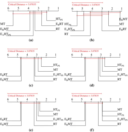
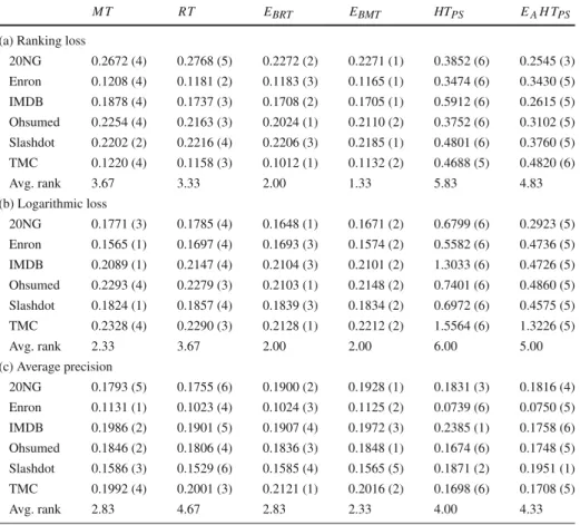
6.3 Results on the ranking-based measures

The performance values and rankings on the ranking-based measures (ranking loss, logarith-mic loss and average precision) are presented in Table5. The results of the Friedman-Nemenyi significance tests are presented in Fig.5. We note that the calculation of logarithmic loss expects the predicted values to lay in the[0,1]interval and that we have no guarantee that the predictions of model trees will fall on this interval. We further discuss the implications of this fact in the discussion section.

6 5 4 3 2 1 HTPS EBRT RT EAHTPS EBMT MT Critical Distance = 3.07835 (a) 6 5 4 3 2 1 EBMT MT EBRT RT EAHTPS HTPS Critical Distance = 3.07835 (b) 6 5 4 3 2 1 HTPS MT EAHTPS RT EBMT EBRT Critical Distance = 3.07835 (c) 6 5 4 3 2 1 HTPS MT EAHTPS RT EBMT EBRT Critical Distance = 3.07835 (d) 6 5 4 3 2 1 HTPS MT E_AHT_PS RT EBMT E_BRT Critical Distance = 3.07835 (e) 6 5 4 3 2 1 MT HTPS E_AHT_PS RT EBMT E_BRT Critical Distance = 3.07835 (f)

Fig. 4 Average ranking diagrams for the label-based measures. a Precisionmacro, b Precisionmicro, cRecallmacro,dRecallmicro,eF1macro,fF1micro

The differences between the results of model and regression trees on the ranking-based evaluation measures are very small. There is variation in which type of tree outperforms the other over the different measures. The average rank of regression trees is slightly higher than that of model trees for ranking loss, while the opposite is true for logarithmic loss and average precision. The differences should be further studied by using pairwise statistical tests. Both iSOUP regression and model trees outperformHTPSin terms of ranking loss and

logarithmic loss (and the difference in performance is statistically significant). In terms of average precision, their results are very close with each of the methods performing best on some of the datasets.

Finally, the ranking diagram for the algorithms in terms of ranking loss shows that bagging with model trees generally performs best on all of the datasets, followed by bagging of regression trees, regression and model trees, and finally EAH TPS andHTPS. In terms of

statistical significance, bagging of model trees is better thanHTPSandEAH TPS, and bagging

Table 5 Predictive performance results: ranking-based measures

M T RT EBRT EBMT HTPS EAH TPS

(a) Ranking loss

20NG 0.2672 (4) 0.2768 (5) 0.2272 (2) 0.2271 (1) 0.3852 (6) 0.2545 (3) Enron 0.1208 (4) 0.1181 (2) 0.1183 (3) 0.1165 (1) 0.3474 (6) 0.3430 (5) IMDB 0.1878 (4) 0.1737 (3) 0.1708 (2) 0.1705 (1) 0.5912 (6) 0.2615 (5) Ohsumed 0.2254 (4) 0.2163 (3) 0.2024 (1) 0.2110 (2) 0.3752 (6) 0.3102 (5) Slashdot 0.2202 (2) 0.2216 (4) 0.2206 (3) 0.2185 (1) 0.4801 (6) 0.3760 (5) TMC 0.1220 (4) 0.1158 (3) 0.1012 (1) 0.1132 (2) 0.4688 (5) 0.4820 (6) Avg. rank 3.67 3.33 2.00 1.33 5.83 4.83 (b) Logarithmic loss 20NG 0.1771 (3) 0.1785 (4) 0.1648 (1) 0.1671 (2) 0.6799 (6) 0.2923 (5) Enron 0.1565 (1) 0.1697 (4) 0.1693 (3) 0.1574 (2) 0.5582 (6) 0.4736 (5) IMDB 0.2089 (1) 0.2147 (4) 0.2104 (3) 0.2101 (2) 1.3033 (6) 0.4726 (5) Ohsumed 0.2293 (4) 0.2279 (3) 0.2103 (1) 0.2148 (2) 0.7401 (6) 0.4860 (5) Slashdot 0.1824 (1) 0.1857 (4) 0.1839 (3) 0.1834 (2) 0.6972 (6) 0.4575 (5) TMC 0.2328 (4) 0.2290 (3) 0.2128 (1) 0.2212 (2) 1.5564 (6) 1.3226 (5) Avg. rank 2.33 3.67 2.00 2.00 6.00 5.00 (c) Average precision 20NG 0.1793 (5) 0.1755 (6) 0.1900 (2) 0.1928 (1) 0.1831 (3) 0.1816 (4) Enron 0.1131 (1) 0.1023 (4) 0.1024 (3) 0.1125 (2) 0.0739 (6) 0.0750 (5) IMDB 0.1986 (2) 0.1901 (5) 0.1907 (4) 0.1972 (3) 0.2385 (1) 0.1758 (6) Ohsumed 0.1846 (2) 0.1806 (4) 0.1836 (3) 0.1848 (1) 0.1674 (6) 0.1748 (5) Slashdot 0.1586 (3) 0.1529 (6) 0.1585 (4) 0.1565 (5) 0.1871 (2) 0.1951 (1) TMC 0.1992 (4) 0.2001 (3) 0.2121 (1) 0.2016 (2) 0.1698 (6) 0.1708 (5) Avg. rank 2.83 4.67 2.83 2.33 4.00 4.33

Each table contains the values of the measure (and the rank) of each method on each dataset

very similar. Here, bagging of model trees, bagging of regression trees, as well as single model trees, statistically significantly outperformHTPS (Fig.5b). The results for average

precision are mixed, with different methods taking first and last rank on different datasets (Fig.5c). Hence, no statistically significant differences were observed.

6.4 Results on the efficiency measures

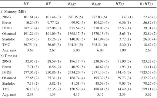
The values and rankings on the efficiency measures (memory and time use) are presented in Table6. The results of the Friedman-Nemenyi significance tests are presented in Fig.6.

The expected result of model trees using both more memory and time is evident from Table6. While the difference in memory use is relatively small, the time use is increased by about 10–20% when using model trees.

HTPSuses considerably less memory when compared to model and regression trees. In

terms of time use, it performs better than iSOUP single trees on some datasets, while it uses considerably more time on others. The differences in time are most likely due to the pruned sets procedure, as the base tree learning steps are similar between the methods.

6 5 4 3 2 1 EBMT EBRT RT MT EAHTPS HTPS Critical Distance = 3.07835 (a) 6 5 4 3 2 1 EBRT EBMT MT RT EAHTPS HTPS Critical Distance = 3.07835 (b) 6 5 4 3 2 1 EBMT MT EBRT HTPS EAHTPS RT Critical Distance = 3.07835 (c)

Fig. 5 Average rank diagrams for the ranking-based measures.aRanking loss,blogarithmic loss,caverage precision

Overall, regression trees appear to be the quickest method, whileHTPSappears to be the

least memory intensive. We observe several statistically significant differences and (even-though some can be inferred by common sense) report all of them. Specifically,HTPSuses

less memory than bagging of regression trees and bagging of model trees, regression trees andEAH TPSuse less memory than bagging of model trees, regression trees are quicker than

bagging of model trees andEAH TPS, and bothM T andHTPSare quicker than EAH TPS

(Fig.6).

6.5 Discussion

We start with a few general remarks, then proceed to address each of the experimental questions in turn.

First, recall that both example-based and label-based measures depend on the selected threshold. While threshold selection is far from a trivial task in the multi-label classification scenario and its difficulty is further compounded in the setting of the data stream mining, it is expected that a better selection of threshold would increase the performance of any classifier. Whether the selection is best done on a method-by-method basis, dataset-by-dataset basis or even for each method-dataset pair requires substantial further investigation. Due to this, we place a stronger emphasis on the threshold-independent ranking-based evaluation measures. We also observe that logarithmic loss is perhaps not the best measure to evaluate model trees and their ensembles in the MLC via MTR setting. The fact that a model tree can predict a value higher than 1 or lower than 0, means that it can be rewarded for predictions for which it is “very sure”, if we look at the predicted value as a probability. However, this cuts both ways, as a prediction of a negative value for a label that is present will also result in a

Table 6 Efficiency results: memory and time usage MT RT EBRT EBMT HTPS EAHTPS (a) Memory (MB) 20NG 101.61 (4) 101.44 (3) 970.35 (5) 972.03 (6) 3.43 (1) 22.46 (2) Enron 10.20 (3) 9.77 (2) 99.92 (5) 104.20 (6) 6.56 (1) 56.82 (4) IMDB 382.33 (4) 382.08 (3) 3575.54 (5) 3578.03 (6) 22.53 (1) 39.31 (2) Ohsumed 191.29 (4) 191.09 (3) 1368.17 (5) 1370.13 (6) 3.63 (1) 32.89 (2) Slashdot 15.45 (3) 15.26 (2) 140.02 (5) 141.94 (6) 3.72 (1) 26.03 (4) TMC 36.75 (4) 36.65 (3) 304.34 (5) 305.31 (6) 2.30 (1) 18.62 (2) Avg. rank 3.67 2.67 5.00 6.00 1.00 2.67 (b) Time (s) 20NG 32.95 (2) 28.59 (1) 196.17 (4) 230.09 (5) 51.90 (3) 723.22 (6) Enron 7.71 (3) 6.56 (2) 40.97 (5) 48.62 (6) 1.93 (1) 13.11 (4) IMDB 277.06 (2) 250.86 (1) 2434.20 (4) 2971.10 (5) 344.45 (3) 4723.53 (6) Ohsumed 27.85 (2) 25.31 (1) 168.74 (4) 195.32 (5) 39.73 (3) 632.72 (6) Slashdot 7.13 (2) 5.82 (1) 41.51 (4) 48.59 (5) 9.03 (3) 78.27 (6) TMC 26.13 (3) 22.35 (2) 150.52 (4) 188.41 (5) 14.49 (1) 259.11 (6) Avg. rank 2.33 1.33 4.17 5.17 2.33 5.67

Each table contains the values of the efficiency measure (and the rank) of each method on each dataset

6 5 4 3 2 1 HTPS RT EAHTPS MT EBRT EBMT Critical Distance = 3.07835 (a) 6 5 4 3 2 1 RT MT HTPS E_BRT EBMT E_AHT_PS Critical Distance = 3.07835 (b)

Fig. 6 Average rank diagrams for the efficiency measures.aMemory consumption,btime consumption more severe penalty in terms of the logarithmic loss. Due to the learning procedure, we do, however, expect that the former will occur more often than the latter.

Regarding the first experimental question, whether model trees with the adaptive per-ceptron outperform regression trees, we can conclude based on the above results that some improvement can be gained by using model trees. However, we also note that using model trees increases the use of resources, which can be a limiting factor when choosing a method for a real-life application. While the increase in memory use is relatively small, model tree construction consumes about 10–20% more time as compared to regression trees.

Continuing to the second question of how iSOUP single model and regression trees compare to Hoeffding trees with pruned sets, we observe that, on the example-based and label-based evaluation measures, all of the trees have similar performance. The only excep-tion is the Hamming score. However, based on the observaexcep-tions made on the ranking-based methods, we conclude that both model and regression iSOUP trees either perform as well as

or outperform the Hoeffding trees with pruned sets, though these findings should be further confirmed by a rigorous statistical testing.

Looking at the results of the comparisons of both single tree and ensemble methods along the various evaluation measures, we find that different methods achieve the best results for different evaluation measures. This is to be expected, as the different learning procedures inevitably optimize different quantities. This in turn influences the performance evaluation for a given evaluation measure, depending on the similarity of the optimized quantity and the evaluation measure.

We did find some statistically significant differences, most notably for the ranking-based ranking loss and logarithmic loss measures. The bagging ensemble of iSOUP model trees outperformed both single tree and ensembles of Hoeffding trees with pruned sets for the first measure and only single Hoeffding trees with pruned sets for the second. These significant differences are very important, as they ranking-based measures in question are threshold independent, while measures like precision and recall can be traded off by setting different thresholds.

Finally, we make conclusions with regard to resource consumption. The results show that, in general, the additional use of resources by the more complex methods, like model trees or ensembles of models, does contribute to better performance. This justifies the use of more complex models. However, we must be aware that there are associated costs that need to be considered. This is especially relevant for real-world applications, where such methods might be made to operate on low-memory or computationally slow devices. To this end, we can recommend the use of memory conservation techniques, such as those proposed by

Ikonomovska et al.(2010).

7 Conclusion and future work

In this paper, we have introduced the multi-label classification via multi-target regression methodology for learning from data streams. We have also introduced the iSOUP-Tree algo-rithm that utilizes this methodology to address the multi-label classification task by using target regression and model trees. We have performed experiments on several multi-label datasets, to address a number of experimental questions concerning the proposed method and its competitors.

First, we have shown that iSOUP model trees is perform better than iSOUP regression trees for a large set of evaluation measures for multi-label classification. For two measures they perform worse. In both cases, the difference is not statistically significant. Th better performance of model trees might be due to the use of the adaptive perceptron. In contrast, in our earlier work the use of regular perceptrons decreased the performance of model trees as compared to the performance of regression trees (Osojnik et al. 2015).

Next, we compared our method in a single tree (non-ensemble) setup to Hoeffding trees with pruned sets (Read et al. 2012). The thresholding aspect of MLC made clear conclusions for some of the observed measures elusive. Still, we can observe that the performance of iSOUP model and regression trees is better than that of Hoeffding trees with pruned sets with respect to two ranking-based measures (ranking loss and logarithmic loss), even though the difference in performance is not statistically significant.

We continued with a wider comparison with some additional methods. Specifically, we included bagging of iSOUP model trees and regression trees, as well as ADWIN bagging of Hoeffding trees with pruned sets. Bagging of iSOUP model trees method performed the best in terms of threshold-independent ranking-based evaluation measures (ranking loss,

logarithmic loss and average precision), with some of the differences in performance being significant. However, further experiments on a larger collection of datasets would be needed to yield stronger statistical confirmation of our findings.

For our experimental comparison, we considered a variety of evaluation measures commonly used in the MLC setting. We obtained the clearest conclusions when using ranking-based measures, which we consider most relevant for MLC, in addition to being threshold-free. However, in real-world applications, any of the considered measures could be a criterion which determines success. The measures we considered are widely used in the MLC community, and showcase the strengths and weaknesses of the observed algorithms.

We have shown that the use of more complex methods yields better predictive performance. However, this comes at the cost of greater use of resources. This should be considered when designing real-world applications, where resources may be limited and a simpler method might be more suitable.

We encountered several interesting avenues of further work. The inescapable problem in multi-label classification is the problem of thresholding. While thresholding is a key piece of the MLC via MTR methodology, it is also present in many methods which directly address the MLC task. Exploring whether a single threshold is appropriate for all of the labels, or whether multiple thresholds, one per label, should be used, is a promising line of future work. Specifically, examining the thresholding strategies ofTsoumakas and Katakis(2007) andLargeron et al.(2012) as well as the work ofTriguero and Vens(2016) and determining if and how their results can be applied in the streaming setting will be our first step along this avenue.

Additionally, we wish to address the task of change detection and adaptation in the iSOUP-Tree method directly, without relying on the use of ensemble methods such as ADWIN bagging. As we have shown, the use of ensembles can incur considerably higher use of resources, which might not be suitable for all applications. We plan to explore both mecha-nisms that deal with targets/labels on a one by one basis, as well as those that consider all of the targets together. The adaptation of approaches for change detection and adaptation from the single-target scenario to the multi-target scenario, e.g., from the work ofIkonomovska et al.(2011b), would be a good first step.

Finally, we plan to extend our MLC via MTR methodology and the iSOUP-Tree method to also address the task of hierarchical multi-label classification (HMC), which is increasingly common in the batch learning scenario. In HMC, the labels are ordered in a hierarchy and adhere to the hierarchy constraint, i.e., if an example is labeled with a label it also has to be labelled with the label’s ancestors. One way to achieve this would be to extend iSOUP-Tree to deal with the task of hierarchical multi-target regression.

Acknowledgements We would like to acknowledge the support of the EC through the projects: MAES-TRA (FP7-ICT-612944) and HBP (FP7-ICT-604102), and the Slovenian Research Agency through a young researcher Grant and the program Knowledge Technologies (P2-0103).

Open Access This article is distributed under the terms of the Creative Commons Attribution 4.0 Interna-tional License (http://creativecommons.org/licenses/by/4.0/), which permits unrestricted use, distribution, and reproduction in any medium, provided you give appropriate credit to the original author(s) and the source, provide a link to the Creative Commons license, and indicate if changes were made.

Appendix: Evaluation measures for multi-label classification

In the following definitions,N is the number of examples in the evaluation sample,Lis the set of all labels andQ = |L|is the number of labels in the provided MLC setting.yˆi and

yialways stand for the predicted scores and actual labelset of theith example, respectively,

though the latter is used interchangeably with it’s indicator vector, i.e., a vector representation of the labelset, where the present labels have a value of 1 while the rest have a value of 0.yˆ andyrefer to a prediction made by a method on some specific (non-indexed) example and its actual labelset, respectively, and are used to define loss functions.yˆ_ijrefers to the predicted score for the jth label, whileyˆ_iλsimilarly refers to the predicted score for the labelλ.

For all example-based and label-based measures,yˆiis assumed to already be thresholded,

i.e.,

ˆ

y_ij=

1; ifyˆ_ij ≥τholds for the predicted scoreyˆ_ij

0; otherwise ,

while the ranking-based measures are computed without thresholding.

Example based measures

Accuracy The accuracy for an example with a predictionyˆand a real labelsetyis defined as the Jaccard similarity coefficient between them, i.e.,| ˆ_{| ˆ}y∩y|_y∪y|. Theaccuracyover a sample is the averaged accuracy over all examples:

Accuracy= 1 N N i=1 | ˆyi∩yi| | ˆyi∪yi|.

The higher the accuracy of a model the better its predictive performance.

F1_{measure. The F}1_{measure for MLC is the natural extension of F}1_{used in regular} classifica-tion, however, we can approach it from either the example-based or label-based perspective. The general formula for calculating F1is the usual harmonic mean of the precision and recall

F1= 2 Precision·Recall Precision+Recall.

If we want to calculate F1from the example-based perspective, we define precision and recall as follows: Precisionex= 1 N N i=1 | ˆyi∩yi| |yi| Recallex = 1 N N i=1 | ˆyi∩yi| | ˆyi| ,

resulting in the final definition for example-based F1measure F1_ex= 2 Precisionex·Recallex

Precisionex+Recallex.

The definitions of the label-based F1measures are found in the following section.

Hamming lossTheHamming lossmeasures how many times an example-label pair is mis-classified. Specifically, each label that is either predicted but not real, or vice versa, carries a penalty to the score. The Hamming loss of a single example is the number of such misclas-sified labels divided by the number of all labels, i.e.,_Q1| ˆyy|whereyˆyis the symmetric difference of the setsyˆandy. The Hamming loss of a sample is the averaged Hamming loss over all examples:

HammingLoss= 1 N N i=1 1 Q| ˆyiyi|.

The Hamming loss of a perfect model, which makes completely correct predictions, is 0 and the lower the Hamming loss the better the predictive performance of a model. Note that the Hamming loss will generally be reported as theHamming score, i.e., HammingScore= 1−HammingLoss.

Label-based measures

To define many of the label-based measures, we expand the definitions of several quantities from regular classification, i.e., the true positive (TP), false positive (FP), true negative (TN) and false negative (FN) rates are each defined on a per-label basis as follows:

TPj=yˆi|lj ∈yi∧lj ∈ ˆyi,1≤i≤N

FPj=yˆi|lj ∈/yi∧lj ∈ ˆyi,1≤i≤N

T Nj=yˆi|lj ∈/yi∧lj ∈ ˆ/yi,1≤i≤N

F Nj=yˆi|lj ∈yi∧lj ∈ ˆ/yi,1≤i≤N,

where 1 ≤ j ≤ Q indexes the labels. This further allows us to extend the definitions of precision, recall and F1in a label-based manner. However, we have two choices how to combine the contributions of each label,macro- andmicro-averaging. In macro-averaging, we compute each measure per label and then average the measures over all of the labels, while in micro-averaging, we first sum up TP, FP, TN and FN values and use those to calculate the measures.

Macro-averaged measuresThe macro-averaged measures are defined as follows: Precisionmacro= 1 Q Q j=1 TPj TPj+FPj Recallmacro= 1 Q Q j=1 TPj TPj+F Nj

To define the macro-averaged F1measure, we further extend the definition by substituting the precision and recall formulas with their forms in terms ofTPj,FPj,T NjandF Nj, resulting

in the formula F1_macro= 1 Q Q j=1 2 TPj TPj+FPj TPj TPj+F Nj TPj TPj+FPj + TPj TPj+F Nj = 1 Q Q j=1 2 2TPj+FPj+F Nj.

Micro-averaged measuresThe following micro-averaged equations are all obtained using the procedure outlined above:

Precisionmicro= Q j=1TPj Q j=1TPj+ Q j=1FPj Recallmicro= Q j=1TPj Q j=1TPj+ Q j=1F Nj F1_micro=2 Precisionmicro·Recallmicro