Nearest Convex Hull Classification
Georgi I. Nalbantov1,2, Patrick J. F. Groenen2, and Jan C. Bioch21 ERIM, Erasmus University Rotterdam 2 Econometric Institute, Erasmus University Rotterdam
Econometric Institute Report EI 2006-50
Abstract. Consider the classification task of assigning a test object to one of two or more possible groups, or classes. An intuitive way to proceed is to assign the object to that class, to which the distance is minimal. As a distance measure to a class, we propose here to use the distance to the convex hull of that class. Hence the name Nearest Convex Hull (NCH) classification for the method. Convex-hull overlap is handled through the introduction of slack variables and kernels. In spirit and computationally the method is therefore close to the popular Support Vector Machine (SVM) classifier. Advantages of the NCH classifier are its robustness to outliers, good regularization properties and relatively easy handling of multi-class problems. We compare the performance of NCH against state-of-art techniques and report promising results.
1
Introduction
There are many approaches to the classification task of separating two or more groups of objects on the basis of some shared characteristics. Existing techniques range from Linear Discriminant Analysis (LDA), Quadratic Discriminant Analy-sis (QDA) and Binary Logistic Regression to Decision Trees, Neural Networks, Support Vector Machines (SVM), etc. Many of those classifiers make use of some kind of a distance metric (in some n-dimensional space) to derive classification rules. Here, we propose to use another such classifier, called Nearest Convex Hull (NCH) classifier.
As the name suggests, the so-called hard-margin version of the NCH classifier assigns a test object x to that group of training objects, which convex hull is closest tox. This involves solving an optimization problem to find the distance to each class. Algorithms for doing so have been proposed in the literature under the general heading of finding the minimum distance between convex sets (see, e.g., [14] and [2]). We confer also to [10] for a more general discussion on distance-based classification. Existing off-the-shelf algorithms however cannot be directly applied for classification tasks where a mixture of a soft-margin and a hard-margin approaches is required. In the separable, hard-hard-margin case, a problem arises if xlies inside the convex hulls of two or more groups, since its distance to these convex hulls is effectively equal to zero and the classification of x is
undetermined. To deal with this problem, we introduce a soft-margin version of the NCH classifier, where convex-hull overlap between x and a given class is penalized linearly. The difference with the soft-margin SVM approach lies in the requirement that the soft approach is applied to all data points except the test pointx. As an alternative solution to convex-hull overlaps, one could map the training data from the original space into a higher-dimensional space where convex-hull overlap can be avoided. A combination of both approaches is also possible.
The linear (and not, for example, quadratic) penalization of the errors gives rise to the robustness-to-outliers property of NCH. Another advantage of NCH in terms of computational speed arises in the context of multi-class classification tasks. This occurs because only same-class objects are considered in the esti-mation of a (soft) distance to a convex hull, and not the whole data set. The decision surface of the NCH classifier is not explicitly computed because the clas-sification process for each test point is independent of the clasclas-sification process for other test points. That is why the classification process is instance-based in nature. In sum, the NCH method can be considered as a type of instance-based large-margin classifier.
The paper is organized as follows. First we provide some intuition behind the NCH classifier and a formal definition of it. Next, we discuss the technical aspects of the classifier – derivation and implementation. Finally, we show some experimental results on popular data sets and then conclude.
2
Nearest Convex Hull Classifier: Definition and
Motivation
At the outset, consider a binary data set of positive and negative objectshI+, I−i
from Rn. Formally, the task is to separate the two classes of objects with a decision surface that performs well on a test data set. This task is formalized as finding a (target) function f :Rn → {−1,1} such that f will classify correctly unseen observations. The extension to the multi-class case is straightforward. The decision rule of the NCH classifier is the following:a test point xshould be assigned to that class, which convex hull is closest to x.
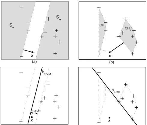
Let us consider the so-called separable case where the classes are separable by a hyperplane and draw an intuitive comparison between NCH and the popular SVM classifier. See Figure 1 for an illustrative binary classification example. Panels (a) and (c) refer to SVM classification, and Panels (b) and (d) refer to NCH classification. In SVM classification, the target function is a hyperplane of the formw0x+b= 0, wherew is a vector of coefficients andbin the intercept.
The SVM hyperplanew∗0x+b∗= 0 (denoted ashSVM) is the one that separates
the classes with the widest margin, where a margin is defined as the distance between a (separating) hyperplane and the closest point to it from the training data set. In terms of Figure 1, Panel (a), the width of white band is equal to twice the margin, which is shown in Panel (c). The closest point to hSVM is defined to lie on the hyperplanew∗0x+b∗= 1 if this point is positively labeled,
S − S + CH − CH + x x h SVM h FCH x x (a) (b) (c) (d) margin
Fig. 1.Classification of a test pointx with SVM in Panels (a) and (c), and NCH in Panels (b) and (d) on a binary data set. In Panel (a), the white band has the largest possible width, which is equal to twice the margin, shown in Panel (c). The points to the left and to the right of the band form shaded sets S− and S+, respectively. Test
point xreceives label +1 since it is farther fromS− thanS+. In Panel (b) pointx is
classified as −1 since it is farther from the convex hull of the positive points, CH+,
than from the convex hull of the negative points,CH−.
or on the hyperplane w∗0x+b∗ =−1 if this closest point is negatively labeled.
For all points xthat lie outside the margin it holds that eitherw∗0x+b∗<−1
or w∗0x+b∗ >1. The former set of points is defined as S
−, and the latter set
of points is defined as S+. For any test pointx, the SVM classification rule can be formulated as follows: a test pointxshould be classified as−1 if it is farther away from setS+ than from setS−; otherwisexreceives label +1.
It has been argued (see, e.g., [4], [14]) that SVM classification searches for a balance between empirical error (or, the goodness-of-fit over the training data) and complexity, where complexity is proxied by the distance between sets S+
andS− (that is, twice the margin). In the separable case at hand, the empirical
error ofhSVMis zero since it fits the data perfectly. Also, complexity and margin width are inversely related: the larger the margin, the lower the associated
com-plexity. The balance between empirical error and complexity can intuitively be approached from an instance-based viewpoint as well. In this case, complexity is imputed in the classification of each separate test object/instance. Thus, the larger the distance from a test object x to the farther one of the two sets S+
andS−, the lower the complexity associated with the classification ofx.
The NCH classifier can also be considered from a fit-versus-complexity stand-point. Let us denote by CH+ and CH− the set of points that form the convex
hulls of the positive and negative objects, respectively (see Figure 1, Panel (b)). Somewhat similarly to SVM, in NCH classification one considers the distance to the farther one of the two convex hullsCH+and CH− as a proxy for the
com-plexity associated with the classification of x. Quite interestingly, this distance is always as big as or bigger than the distance from xto the farther of setsS+
and S−. This property holds since the convex hull of the +1 (−1) points is a
subset of S+ (S−), as can be seen in Figure 1. Therefore, if one considers the
distance to the farther-away convex hull as a proxy for complexity associated with the classification ofx, then NCH classification is characterized by a lower complexity than SVM classification. However, the fit over the training data of NCH may turn out to be inferior to SVM in some cases. Let hFCH denote the hyperplane that is tangent to the farther-away convex hull of same-class train-ing data points, and is perpendicular to the line segment that represents the distance between x and this convex hull, as in Figure 1, Panel (d). Thus, the distance between x and hFCH equals the distance between x and the farther convex hull. Effectively, in NCH classification xis classified usinghFCH. Notice that by definition hFCH separates without an error either the positive or the negative observations, depending on which convex hull is farther from x. Thus,
hFCHis not guaranteed to have a perfect fit over the whole data set that consists of both positive and negative points, as illustrated in Figure 1, Panel (d). As a consequence, it is not clear a priory whether NCH or SVM will strike a better balance between fit and complexity in the classification of a given pointx: there is a gain for NCH coming from decreased complexity (in the form of an increased distance) vis-a-vis SVM on the one hand, accompanied by a potential loss arising from a possible increased empirical error ofhFCH over the whole training data
set, on the other.
NCH has the property that the extent of proximity to a given class is deter-mined without taking into consideration objects from other classes. This prop-erty contrasts with the SVM approach, where the setsS+andS−are not created
independently of each other. A similar parallel can be drawn between LDA and QDA methods. In LDA, one first determines the Mahalanobis distances fromx to the centers of the classes using a common pooled covariance matrix and then classifiesxaccordingly. In QDA, one uses a separate covariance matrix for each class. Analogically, the NCH classifier first determines the Euclidean distance from x to the convex hulls of each of the classes and then classifiesx accord-ingly. In sum, loosely speaking one may think of the shift from SVM to NCH as resembling the shift from LDA to QDA.
x x x
(a) (b) (c)
a b
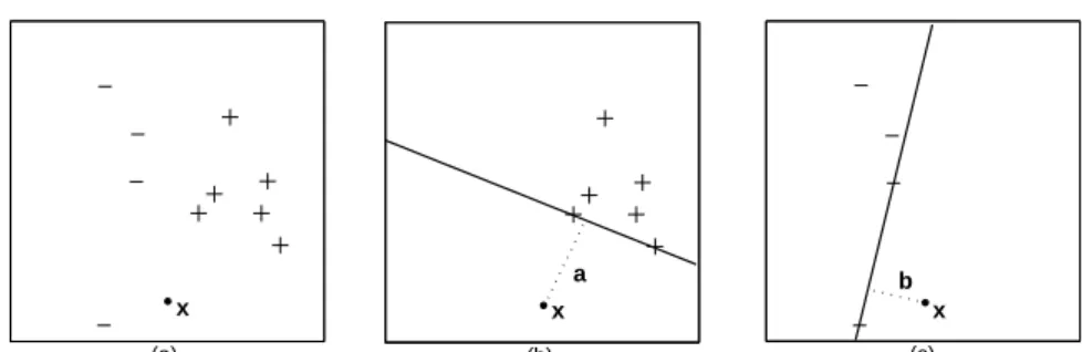
Fig. 2.Classification of a test pointxwith NCH on the binary data set in Panel (a) in two steps. At stage one (Panel (b)), a test pointxis added to a data set that contains only the positive class, and the distance a fromx to the convex hull of this class is computed. At stage two (Panel (c)),x is added to a data set that contains only the negative class, and the distancebfromxto the convex hull of this class is computed. If a>b(a<b), thenxis assigned to the negative (positive) class.
3
Estimation
3.1 Separable caseConsider a data set oflobjects fromkdifferent groups, or classes. Letlk denote the number of objects in the kth class. According to NCH, a test point x is assigned to that class, to which the distance is minimal. In the separable case, the distance to a class is defined as the distance to the convex hull of the objects from that class. The algorithm for classifyingxcan be described as follows (see Figure (2)): first, compute the distance fromxto the convex hull of each of the
kclasses; second, assign to xthe label of the closest class. Formally, to find the distance from a test pointxto the convex hull of the nearest class, the following quadratic optimization problem has to be solved for each classk:
min wk,bk 1 2w 0 kwk (1) such that wk0xi+bk ≥0, i= 1,2, . . . , lk −(w0 kx+bk) = 1 The distance between hyperplanew0
kx+bk = 0 andxis defined as 1/
p
w0
kwk by the last constraint of (1). This distance is maximal when 1
2wk0wk is minimal. At the optimum, it represents the distance fromxto the convex hull of classk. The role of the first lk inequality constraints is to ensure that the hyperplane classifies correctly each point that belongs to classk. Effectively, for each of the
k classes, the lk same-class objects are assigned label 1, and the test point is assigned label−1. Eventually,xis assigned to that class to which the distance is minimal, that is, which corresponding value for the objective function in (1) is maximal.
3.2 Nonseparable case
Optimization problem (1) can be solved for each k only if the test point lies outside the convex hull of each classk. A further complication arises if some of the convex hulls overlap. Then a test point could lie simultaneously in two or more convex hulls and its classification label would be undetermined. To cope with these situations, so-called slack variables can be introduced, similarly to the SVM approach. Consequently, the nonseparable version of optimization problem (1) that has to be solved for each classk becomes:
min wk,bk,ξ 1 2w 0 kwk+C lk X i=1 ξi (2) such that. wk0xi+bk ≥0−ξi, ξi≥0, i= 1,2, . . . , lk −(w0 kx+bk) = 1.
Note that in (2) the points that are incorrectly classified are penalized linearly via the termPlki=1ξi. If one prefers a quadratic penalization of the classification errors, then the sum of squared errorsPlki=1ξ2
i should be substituted for
Plk
i=1ξi in (2). One can go even further and extend the NCH algorithm in a way analogical to LS-SVM ([7]) by imposing in (2) that constraintsw0
kxi+bk ≥0−ξihold as equalities, on top of substitutingPlki=1ξ2
i for
Plk i=1ξi.
Each of thek (primal) optimization problems pertaining to (2) can be ex-pressed in dual form1as:
max α αlk+1− 1 2 Plk+1 i,j=1αiαjyiyj(x0ixj) (3) such that 0≤αi ≤C, i= 1,2, . . . , lk, and
Plk+1
i=1 yiαi= 0,
where theα’s are the Lagrange multipliers associated with the respectivekth pri-mal problem. Here αlk+1 is the Lagrange multiplier associated with the
equal-ity constraint −(w0
kx+bk) = 1. In each problem yi = 1, i = 1,2, . . . , lk and
ylk+1=−1. The advantage of the dual formulation (3) is that differentMercer
kernels can be employed to replace the inner product x0
ixj in (3) in order to obtain nonlinear decision boundaries, just like in the SVM case. Three popular kernels are linearκ(xi,xj) =x0ixj, polynomial of degreed κ(xi,xj) = (x0ixj+1)d and the Radial Basis Function (RBF) kernel κ(xi,xj) = exp(−γ kxi−xj k2), where the manually-adjustable γ parameter determines the proximity between xi andxj.
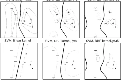
A total ofkNCH optimization problems have to be solved to determine the class of any test pointx. This property provides for the fact that the NCH deci-sion boundary is in general implicit and nonlinear, even in case the original data is not mapped into a higher-dimensional space via a kernel. Figure 3 demon-strates that this property does not hold in general for Support Vector Machines, 1 The derivation of the dual problem resembles the one used in SVM (see, e.g., [4]).
NCH, linear kernel NCH, RBF kernel, γ=5 NCH, RBF kernel,γ=35
SVM, RBF kernel,γ=35 SVM, RBF kernel, γ=5
SVM, linear kernel
Fig. 3.Decision boundaries for NCH and SVM using the linear and RBF kernels on a linearly separable data set. The dashed contours for the NCH method are iso-curves along which the ratio of the distances to the two convex hulls is constant.
for instance. This figure also illustrates that the NCH decision boundary ap-pears to be less sensitive to the choice of kernel and kernel parameters than the respective SVM boundary.
Technically speaking, in case the convex hulls do not overlap, NCH could be solved using the standard SVM optimization formulation (see, e.g., [14], [4]). In this case one searches for the widest margin between each of the k classes and a test pointx. This margin represents the distance fromxto the convex hull of thekthclass. The class for which the margin is smallest is the winning one. The standard nonseparable-case SVM formulation cannot however be automatically applied to the nonseparable NCH case, since the equality constraint in (2) will not be satisfied in general.
4
Experiments on Some UCI and SlatLog Data Sets
The basic optimization algorithm for Nearest Convex Hull classification (3) is implemented via a modification of the freely available LIBSVM software ([5]). We tested the performance of NCH on several small- to middle-sized data sets that are freely available from the SlatLog and UCI repositories ([12]) and have been analyzed by many researchers and practitioners (e.g. [3], [8], [9], [13] and others): Sonar, Voting, Wisconsin Breast Cancer (W.B.C.), Heart, Australian Credit Approval (A.C.A.), and Hepatitis (Hep.). Detailed information on these data sets can be found on the web sites of the respective repositories.We compare the results of NCH to those of several state-of-art techniques: Support Vector Machines (SVM), Linear and Quadratic Discriminant Analysis
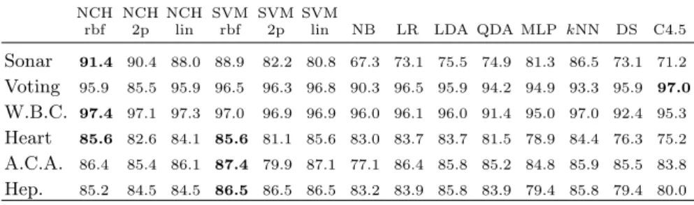
Table 1.Leave-one-out accuracy rates (in %) of the Nearest Convex Hull classifier as well as some standard methods on several data sets. Rbf, 2p and lin stand for Radial Basis Function, second-degree polynomial and linear kernel, respectively
NCH NCH NCH SVM SVM SVM
rbf 2p lin rbf 2p lin NB LR LDA QDA MLP kNN DS C4.5
Sonar 91.4 90.4 88.0 88.9 82.2 80.8 67.3 73.1 75.5 74.9 81.3 86.5 73.1 71.2 Voting 95.9 85.5 95.9 96.5 96.3 96.8 90.3 96.5 95.9 94.2 94.9 93.3 95.9 97.0 W.B.C. 97.4 97.1 97.3 97.0 96.9 96.9 96.0 96.1 96.0 91.4 95.0 97.0 92.4 95.3 Heart 85.6 82.6 84.1 85.6 81.1 85.6 83.0 83.7 83.7 81.5 78.9 84.4 76.3 75.2 A.C.A. 86.4 85.4 86.1 87.4 79.9 87.1 77.1 86.4 85.8 85.2 84.8 85.9 85.5 83.8 Hep. 85.2 84.5 84.5 86.5 86.5 86.5 83.2 83.9 85.8 83.9 79.4 85.8 79.4 80.0
(LDA and QDA), Logistic Regression (LR), Multi-layer Perceptron (MLP), k -Nearest Neighbor (kNN), Naive Bayes classifier (NB) and two types of Decision Trees – Decision Stump (DS) and C4.5. The experiments for the NB, LR, MLP,
kNN, DS and C4.5 methods have been carried out with the WEKA learning environment using default model parameters, except forkNN. We refer to [15] for additional information on these classifiers and their implementation. We measure model performance by the leave-one-out (LOO) accuracy rate. Because we aim at comparing several methods, LOO seems to be more suitable than the more generalk-fold cross-validation (CV), because it always yields one and the same error rate estimate for a given model, unlike the CV method (which involves a random split of the data into several parts).
Table 1 presents performance results for all methods considered. Some meth-ods, namelykNN, NCH and SVM, require tuning of model parameters. In these cases, we report only the highest LOO accuracy rate obtained by performing a grid search for tuning the necessary parameters. Overall, the NCH classifier performs quite well on all data sets, and achieves best accuracy rates on three data sets. SVM also perform best on three data sets. The rest of the techniques show relatively less favorable and more volatile results. For example, the C4.5 classifier performs best on theVotingdata set, but achieves rather low accuracy rates on two other data sets –Sonar andHeart. Note that not all data sets are equally easy to handle. For instance, the performance variation over all classifiers on the Voting andBreast Cancer data sets is rather low, whereas on the Sonar data set it is quite substantial.
5
Conclusion
We have introduced a new technique that can be considered as a type of an instance-based large-margin classifier, called Nearest Convex Hull classifier (NCH). NCH assigns a test observation to the class, which convex hull is closest. Convex-hull overlap is handled via the introduction of slack variables and/or ker-nels. NCH induces an implicit and generally nonlinear decision surface between
the classes. One of the advantages of NCH is that an extension from binary to multi-class classification tasks can be carried out in a straightforward way. Others are its alleged robustness to outliers and good generalization qualities. A potential weak point of NCH, which also holds for SVM, is that it is not clear a priori which type of kernel and what value of the tuning parameters should be used. Furthermore, we do not address the issue of attribute selection and the estimation of class-membership probabilities. Further research could also con-centrate on the application of NCH in more domains, on faster implementation suitable for analyzing large-scale data sets, and on the derivation of theoretical test-error bounds.
References
1. Ben-Hur, A., Horn, D., Siegelmann, H.T., Vapnik V.: Support Vector Clustering. Journal of Machine Learning Research2(2001) 125–137
2. Bennett, K., Bredensteiner, E.: Duality and Geometry in SVM Classifiers. In Pro-ceeddings of the 17th International Confefence on Machine Learning, Morgan Kauf-mann, San Francisco, CA, (2000) 57–64
3. Breiman, L.: Bagging predictors. Machine Learning24(1996) 123–140
4. Burges, C.: A tutorial on support vector machines for pattern recognition. Data Mining and Knowledge Discovery2(1998) 121–167
5. Chang, C.C., Lin, C.J.: LIBSVM: a library for support vector machines (2006) Software available athttp://www.csie.ntu.edu.tw/∼cjlin/libsvm.
6. Cristianini, N., Shawe-Taylor, J.: An Introduction to Support Vector Machines. Cambridge University Press (2000)
7. van Gestel, T.V., Suykens, J.A.K., Baesens, B., Viaene, S., Vanthienen, J., De-dene, G., Moor, B.D., Vandewalle, J.: Benchmarking least squares support vector machine classifiers. Machine Learning 24(2004) 5–32
8. King, R.D., Feng, C., Sutherland, A.: STATLOG: comparison of classification al-gorithms on large real-world problems. Applied Artificial Intelligence 9(3)(1995) 289–334
9. Lim, T., Loh, W., Shih, Y.: A comparison of prediction accuracy, complexity, and training time for thirtythree old and new classification algorithms. Machine Learning40(1995) 203–228
10. von Luxburg, U., Bousquet, O.: Distance–Based Classification with Lipschitz Func-tions. Journal of Machine Learning Research5(2004) 669–695
11. Nalbantov, G.I., Bioch, J.C., Groenen, P.J.F.: Instance-based classification with support hyperplanes. Econometric Institute technical report, Erasmus University Rottedam (to appear)
12. Newman, D., Hettich, S., Blake, C., Merz, C.: UCI Repository of machine learning databases (1998)http://www.ics.uci.edu/∼mlearn/MLRepository.html
Univer-sity of California, Irvine, Dept. of Information and Computer Sciences.
13. Perlich, C., Provost, F., Simonoff, J.S.: Tree induction vs. logistic regression: a learning-curve analysis. Journal Of Machine Learning Research4(2003) 211–255 14. Vapnik, V.N.: The Nature of Statistical Learning Theory. Springer-Verlag New
York, Inc. (1995) 2nd edition, 2000.
15. Witten, I.H., Frank, E.: Data Mining: Practical machine learning tools and tech-niques. Morgan Kaufman, San Francisco (2005) 2nd edition.