Optimization of a Coded-Modulation System with Shaped Constellation

(1)

Graduate Theses, Dissertations, and Problem Reports 2013

Optimization of a Coded-Modulation System with Shaped

Constellation

Xingyu Xiang

West Virginia University

Follow this and additional works at: https://researchrepository.wvu.edu/etd

Recommended Citation Recommended Citation

Xiang, Xingyu, "Optimization of a Coded-Modulation System with Shaped Constellation" (2013). Graduate Theses, Dissertations, and Problem Reports. 207.

https://researchrepository.wvu.edu/etd/207

This Dissertation is protected by copyright and/or related rights. It has been brought to you by the The Research Repository @ WVU with permission from the rights-holder(s). You are free to use this Dissertation in any way that is permitted by the copyright and related rights legislation that applies to your use. For other uses you must obtain permission from the rights-holder(s) directly, unless additional rights are indicated by a Creative Commons license in the record and/ or on the work itself. This Dissertation has been accepted for inclusion in WVU Graduate Theses, Dissertations, and Problem Reports collection by an authorized administrator of The Research Repository @ WVU. For more information, please contact [email protected].

(2)

Optimization of a Coded-Modulation System

with Shaped Constellation

by Xingyu Xiang

Dissertation submitted to the

College of Engineering and Mineral Resources at West Virginia University

in partial fulfillment of the requirements for the degree of

Ph.D. in Electrical Engineering Brian D. Woerner, Ph.D. Daryl S. Reynolds, Ph.D. John Goldwasser, Ph.D. Natalia A. Schmid, Ph.D. Matthew C. Valenti, Ph.D., Chair

Lane Department of Computer Science and Electrical Engineering

Morgantown, West Virginia 2013

Keywords: Information Theory, Constellation Shaping, Capacity, LDPC code, Optimization, EXIT chart

(3)

Abstract

Optimization of a Coded-Modulation System with Shaped Constellation by

Xingyu Xiang

Ph.D. in Electrical Engineering West Virginia University Matthew C. Valenti, Ph.D., Chair

Conventional communication systems transmit signals that are selected from a signal constellation with uniform probability. However, information-theoretic results suggest that performance may be improved by shaping the constellation such that lower-energy signals are selected more frequently than higher-energy signals. This dissertation presents an energy-efficient approach for shaping the constellations used by coded-modulation systems. The focus is on designing shaping techniques for systems that use a combination of amplitude-phase shift keying (APSK) and low-density parity check (LDPC) coding. Such a combination is typical of modern satellite communications, such as the system used by the DVB-S2 standard.

The system implementation requires that a subset of the bits at the output of the LDPC encoder are passed through a nonlinear shaping encoder whose output bits are more likely to be a zero than a one. The constellation is partitioned into a plurality of sub-constellations, each with a different average signal energy, and the shaping bits are used to select the sub-constellation. An iterative receiver exchanges soft information among the demodulator, LDPC decoder, and shaping decoder. Parameters associated with the modulation and shap-ing code are optimized with respect to information rate, while the design of the LDPC code is optimized for the shaped modulation with the assistance of extrinsic-information transfer (EXIT) charts. The rule for labeling the constellation with bits is optimized using a novel hybrid cost function and a binary switching algorithm.

Simulation results show that the combination of constellation shaping, LDPC code op-timization, and optimized bit labeling can achieve a gain in excess of 1 dB in an additive white Gaussian noise (AWGN) channel at a rate of 3 bits/symbol compared with a system that adheres directly to the DVB-S2 standard.

(4)

iii

Acknowledgements

This dissertation could never be finished without the assistants and contributions from a great many people around. I would like to extend my appreciation especially to the following. First and foremost, my deepest gratitude is to my dissertation committee chairman and advisor, Dr. Matthew C. Valenti, who is my first foreign advisor and also the best advisor I have ever met. I can still remember the exciting scene that I received the email from Dr. Valenti about his research plan together with the official invitation. His excellent guidance, patience, and enthusiasm attitude made me overcome the problems came across the whole graduate career. He provides the support in almost every possible way, I appreciate his time, idea, editing and funding in the completion of this and other documents. It is an honor to work with him and his instructions will continue benefit my future lives.

To the other members of my committee, Dr. Brian Woerner, Dr. Daryl Reynolds, Dr. Natalia Schmid and Dr. John Goldwasser, thank you for your feedback and suggestions to make this dissertation more thorough and rigorous.

I spend most of my professional and personal time in the wireless communication research lab, from where I obtain both friendship and illuminating advice. I am grateful for the colleagues who stayed with me in the past few years: Terry R. Ferret, Mohammad Fanaei, Salvatore Talarico, Aruna Sri and Chandana Nannapaneni. Particularly I would like to acknowledge Terry for helping me settle down on my first day of arrival, he also help Dr. Valenti to maintain the cluster system to provide us the extra computing power. Without all of their contributions to the grid computing, the results of this dissertation would take much more time to be finished. Other graduate students that I have had the pleasure to be alongside of are Jinyu Zuo, Ricky Hussmann, Yuan Li and Wentian Zhou.

My time at West Virginia University was enjoyable due to the beautiful environment and the unique graduate student experience, it becomes a part of my life and thanks to all the professors and friends to make it memorable. Special recognition goes out to my family I

(5)

ACKNOWLEDGEMENTS iv would like thank my parents for all their love and encouragement. They supported me and trusted me unconditionally even in the tough times. Lastly, I want to thank the WVU staff and my friends in China, America and elsewhere for their support and encouragement.

(6)

iv

List of Figures

1.1 Block diagram for a basic digital communication system. . . 2

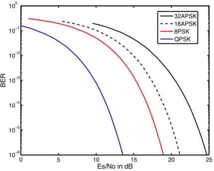
1.2 Bit Error Rate of Uncoded Modulations . . . 5

1.3 Convolutional encoder . . . 6

1.4 Structure of turbo encoder . . . 7

1.5 Structure of turbo decoder . . . 8

1.6 Tanner Graph corresponding to H1, the squares represent check nodes and the circles represent check nodes. . . 11

1.7 16-APSK . . . 18

1.8 Caption for LOF . . . 19

1.9 Distorted 16-QAM on the outputs of non-linear TWTA . . . 20

1.10 Distorted 32-APSK on the outputs of non-linear TWTA . . . 20

1.11 Magnitude Predistortion linearizers generate a response opposite to a TWTA’s characteristics . . . 21

1.12 Phase Predistortion linearizers generate a response opposite to a TWTA’s characteristics . . . 21

1.13 Predistorted QAM and 32-APSK on the outputs of non-linear TWTA . . . . 22

1.14 Performance of DVB-S2 standardized LDPC coded over AWGN channel . . . 23

1.15 Caption for LOF . . . 24

2.1 Unconstrained AWGN channel capacity and SIR with equiprobable M-QAM(PSK) inputs . . . 32

2.2 A BICM system structure which contains the CM system. The block ‘Enc’ is the binary channel encoder, ‘Π’ is a bit-level interleaver and ‘Φ’ is a memory-less mapper. The blocks at the receiver side are the reverse processes. . . 32

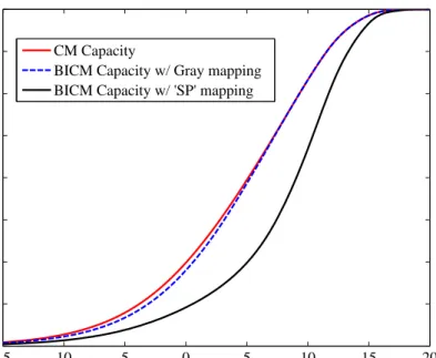
2.3 CM and BICM capacity for 16-QAM with uniform distribution, the BICM capacities are generated with two labeling rules . . . 34

2.4 Information rate results of uniform 32-APSK modulation generated by two methodologies . . . 37

2.5 Transmitter structure. . . 38

2.6 16-PAM constellation. . . 41

2.7 16-APSK constellation. . . 42

(9)

LIST OF FIGURES vii 2.9 Information rate (in bits per channel use) of 16-APSK ,16-PAM and 32-APSK

with uniform input distributions over AWGN and ergodic Rayleigh fading channels. The rates for APSK modulation are maximized over the permissible

ring radius ratios. . . 45

2.10 Information rate of nonuniform APSK and 16-PAM. The number of shaping bit used is indicated. The solid black line on the right of each subfigure corresponds to a uniform input distribution. The results of AWGN Channel are shown in the first row, the results of ergodic Rayleigh fading channel are shown in the second row. Subfigures in leftmost column: 16-APSK with 1 or 2 shaping bits. Subfigures in the middle column: 16-PAM with 1 or 2 shaping bits. Subfigures in last column: 32-APSK with 1, 2, or 3 shaping bits. . . 47

2.11 Shaping gain of 16-PAM, 16-APSK and 32-APSK over AWGN and ergodic Rayleigh fading channel. For 16-PAM and 32-APSK, 1 shaping bits are used. For 16-APSK, 2 shaping bits are used . . . 49

2.12 The value ofp0 that maximizes the information rate for nonuniform APSK in AWGN and ergodic Rayleigh fading. For 16-APSK, 2 shaping bits are used, while for 16-PAM and 32-APSK, 1 shaping bit is used. . . 50

2.13 Peak-to-average power ratio (PAPR) of nonuniform 16-PAM, 32-APSK and 16-APSK as a function of p0 and the number of shaping bits. For 16-APSK, γ = 2.57, and for 32-APSK, γ ={2.64,4.64}. . . 51

3.1 32-APSK constellation. . . 55

3.2 Receiver structure. . . 56

3.3 Turbo decoder . . . 61

3.4 LDPC decoder . . . 62

3.5 Bit-error rate of 16-PAM in AWGN and fading channel . . . 66

3.6 Bit-error rate of 32-APSK in AWGN and fading channel . . . 67

3.7 Bit-error rate of LDPC-coded 16-PAM at rate R = 3 bits/symbol both with and without shaping. Curves are shown for AWGN and Rayleigh Fading channel. . . 68

3.8 Bit-error rate of LDPC-coded 32-APSK in AWGN at rateR = 3 bits/symbol both with and without shaping. Curves are shown for the unshaped (uniform) system using BICM and BICM-ID. Curves are shown for three shaping codes, and the shaped system uses BICM-ID. . . 69

3.9 Bit-error rate for the same system described in Fig. 3.2 in fully-interleaved Rayleigh fading. . . 70

3.10 Average number of BICM-ID global iterations required for correcting all code-word errors. . . 71

4.1 Demodulator mutual information transfer characteristics for 16-QAM with ’SP’ labeling . . . 75

4.2 Demodulator mutual information transfer characteristics for different 16-QAM mappings atEs/N0 = 4.5dB . . . 76

4.3 Decoder mutual information transfer characteristics for rate 1/2 convolutional code with different code memory . . . 77

(10)

LIST OF FIGURES viii 4.4 EXIT chart for 16-QAM modulation with ’SP’ mapping at Es/N0 = 6dB,

averaged decoding trajectories are also shown . . . 78 4.5 VND curves for LDPC codes over AWGN channel . . . 80 4.6 CND EXIT curves . . . 80 4.7 Exit chart for the uniform system with DVB-S2 standard LDPC code and

32-APSK modulation atEb/N0 = 4.93 dB . . . 82

4.8 EXIT chart for BICM-ID using M=32 APSK and overall system rate R=3.85 over AWGN channel at Eb/N0 = 7dB. Different decoder characteristic curves

correspond various channel decoder iterations. From left to right, the six decoder curves correspond to 1 through 6 iterations. . . 84 4.9 EXIT chart for the shaped system described in chapter 3 using M=32 APSK

and overall system rate R=3 over AWGN channel at Eb/N0 = 4.76dB. . . . 85

4.10 Curve fit for an LDPC code at code rate R = 3/5 with uniform 32-APSK constellation,Eb/N0 = 4.5dB . . . 88

4.11 Bit-error rate of 32-APSK in AWGN at rateR = 3 bits/symbol with a length nc = 64 800 LDPC code. The solid lines are for the uniform system; the

rightmost curve shows the performance of uniform modulation with a standard DVB-S2 code, while the two curve to its left show the performance of uniform modulation with optimized D = 3 and D = 4 LDPC codes, respectively. The dashed lines are for the shaped system; with the left two curves show the performance of shaped modulation with optimized D = 3 and D = 4 LDPC codes, and the third curve from left shows the performance of shaped modulation with a standard DVB-S2 code . . . 89 4.12 EXIT chart for BICM-ID using M=32 APSK and overall system rate R=3

over AWGN channel atEb/N0 = 4.73dB. . . 91

4.13 Bit-error rate of 32-APSK in AWGN at rate R = 3 bits/symbol with short length LDPC codes (nc = 16 200). The solid lines are for the uniform system;

from right to left, the curves show uniform system using Rc = 3/5 DVB-S2

standard code, uniform system with optimized code with D = 3 and D= 4. The dashed lines are for the shaped system; from left to right, the curves show performance using optimized Rc = 9/14 LDPC code with D = 4 and

D= 3 combined with (3,2) shaping code, the third curve from left shows the performance of standardRc= 2/3 code with (4,2) shaping code . . . 92

4.14 Bit-error rate of 32-APSK in ergodic Rayleigh fading channel at rate R = 3 bits/symbol with a length nc = 64 800 LDPC code. The three curves on the

right side are for the uniform system, the three curves on the left side are for the shaped systems. . . 94 4.15 Bit-error rate of 32-APSK in ergodic Rayleigh fading channel at rate R = 3

bits/symbol with a lengthnc= 64 800 LDPC code. The solid lines are for the

uniform system, The dashed lines are for the shaped system. . . 95 4.16 The form of a 4 cycle in a parity-check matrix . . . 96 4.17 Bit-error rate of shaped 32-APSK at rate R = 3 bits/symbol with a length

nc= 64 800 LDPC code over AWGN channel. The solid lines are results with

the LDPC codes without 4 cycles, the dashed lines are for the LDPC codes with 4 cycles. . . 97

(11)

LIST OF FIGURES ix 5.1 Four mappings of 8-PSK constellation . . . 101 5.2 16-APSK with mapping defined in DVB-S2 standard. Decision regions for

bit m = 1,2,3,4 with no a priori information. Shaded region is the decision region where bitm is 0 . . . 102 5.3 The 16-APSK symbol with label (0000) is transmitted, decision regions for

the first bit equals to 0 when 1,2,3 bits are known, respectively. The labeling is from DVB-S2 standard. . . 103 5.4 Bit-error rate of 8-PSK in AWGN at rate R = 2 bits/symbol with a length

nc = 64 800 DVB-S2 LDPC code over AWGN channel. The dashed lines are

for the uniform BICM systems; the solid lines are for the BICM-ID uniform system. . . 105 5.5 Bit-wise mutual information of 8-PSK with different mapping rules . . . 110 5.6 Bit-wise mutual information of 8-PSK with different mapping rules . . . 112 5.7 BER of 32-APSK in AWGN at rate R = 3 bits/symbol with a length nc =

64 800 DVB-S2 LDPC code. The dashed lines are the results with optimized mapping rule; the solid lines are for the system with DVB-S2 standard map-ping rule. . . 113 5.8 Optimized Mapping of 32-APSK for shaped system . . . 114 5.9 Bit-error rate of shaped 32-APSK in AWGN at rateR = 3 bits/symbol. The

LDPC code has rate 2/3 and length nc = 64 800 LDPC codes. The (4,2)

shaping code is used. . . 114 5.10 Demodulator mutual information transfer characteristic for uniform 32-APSK

atEb/N0 = 5 dB . . . 116

5.11 Bit-error rate of 32-APSK in AWGN channel at rate R= 3 bits/symbol. The length of LDPC code is kept to be nc= 64 800 . . . 118

5.12 Gradient-search algorithm derived M = 32 signal constellation . . . 120 5.13 Bit-error rate of 32-APSK in AWGN at rateR = 3 bits/symbol with a length

nc = 64 800 DVB-S2 LDPC code over AWGN channel. The dashed lines are

for the BICM systems; the solid lines are for the BICM-ID system. . . 121 5.14 Gray 32-APSK with 2 rings . . . 122

(12)

x

List of Tables

2.1 Minimum requiredEb/N0 in AWGN for 16-PAM and M-APSK withg shaping

bits. The optimizing p0 and γ are shown. . . 48

2.2 Minimum requiredEb/N0in ergodic Rayleigh fading for 16-PAM and M-APSK

with g shaping bits. The optimizingp0 and γ are shown. . . 48

3.1 Parameters used for the systems with turbo code . . . 65 5.1 Values of Cost Functions related to Euclidean distance at Es/N0 = 8 dB. . . 108

(13)

1

Chapter 1

Introduction

Digital communication is responsible for the transmission of useful data to one or more destinations through physical media or channels. Channel capacity is the highest information rate that can be transmitted reliably over a communication channel with arbitrarily small error probability [1]. The capacity value is given by the maximum of the mutual information between the input and output signals of the channel, where the maximization is with re-spect to the input distribution. The difference between the reliable system transmission rate and channel capacity becomes an important criteria to benchmark practical systems. Mod-ern channel coding, e.g. turbo codes [2] and Low Density Parity Check (LDPC) codes [3, 4] approach channel capacity closely. When combined with other digital communication strate-gies, the system could perform even better. The work described in the following chapters is about certain optimization strategies to improve the performance of digital communications. This chapter begins with an introduction to the basic components of digital commu-nication systems. Channel coding, including turbo and LDPC codes, are briefly reviewed since they are a critical component of the systems implemented later in this dissertation. Next, satellite communication systems, including the Digital Video Broadcasting - Second Generation (DVB-S2) standard, are discussed with an emphasis on their performances. The last part is an overview of the reminder of the dissertation.

(14)

Xingyu Xiang Chapter 1. Introduction 2 Channel Source Source Channel Encoder Modulator Source Encoder Source Channel Demodulator Channel Decoder Source Decoder Sink

Figure 1.1: Block diagram for a basic digital communication system.

1.1

Digital Communication System Model

An elementary block diagram of a digital communication system is shown in Fig. 1.1. The aim of the communication system is for the sink to recover the messages from the source with certain reliability. The source is generally considered as a sequence of bits drawn according to a probabilistic model. The source encoder converts the information source sequence into an alternative sequence which is a more efficient representation. It compresses the information sequence into a shorter sequence using certain algorithms or coding strategies. Depending on the requirements of the application, the compression can be either lossless or lossy. The output of source encoder is sent to the channel encoder, which adds controlled redundancy that can be used by the receiver to detect and correct errors caused by the channel.

The modulator maps the output of channel encoder onto analog waveforms chosen from

a finite set according to mapping and labeling rules. The modulated waveforms are then transmitted through channels that are corrupted by distortion and noise. Physical medi-ums like the atmosphere, wire lines, optical fibre, and other medimedi-ums could be used as the communication channel. The demodulator collects the distorted signals and computes an estimate of the probabilities of the modulated symbols. The output of the demodulator is sent to thechannel decoder, which reduces the number of errors induced by the channel with the assistance of the redundancy introduced by the channel encoder. The source decoder decompresses and reconstructs the message, which is delivered to the sink. The difference or functions of the difference between the original signal and the reconstructed signal is a measure of the distortion or the demodulator-detector performance.

(15)

Xingyu Xiang Chapter 1. Introduction 3 An actual digital communication system is far more sophisticated than the generalized description above. Some systems contain an amplifier in the transmitter or a quantizer at the input to the receiver. In addition, in some systems the demodulator and channel decoder work jointly or iteratively to recover the message.

1.2

Modulation

Analog modulation and digital modulation are the two basic types of modulation. Ana-log modulation uses anaAna-log information to modulate a carrier by using it to change the amplitude, frequency, phase, or some combination of the three. Demodulators for analog modulation are simple and cheap to implement, but analog modulation requires lots of power and is vulnerable to noise and distortion. The move from analog modulation to digital mod-ulation provides more information capacity, compatibility with digital data services, higher data security and better quality communications. In digital modulation systems, an analog carrier is modulated by a discrete signal and the modulation can be considered as digital-to-analog conversion; the corresponding demodulation or detection is responsible for the opposite analog-to-digital conversion. For a wireless communication channel, the input bit stream must be represented by a high-frequency signal to facilitate transmission with an antenna of reasonable size.

Most communication systems belong to one of three categories: bandwidth efficient, power efficient, or cost efficient. Bandwidth efficiency or spectral efficiency refers to the ability to transmit at a high information rate over a limited bandwidth. Power efficiency describes the ability of the system to reliably send information at the lowest practical power level. The parameters to be optimized depend on the particular system. For digital terrestrial microwave radios, the bandwidth efficiency might be the highest priority factor, but power efficiency may be more important for the hand-held cellular phones since they need to run on a battery and for satellite communication systems, which must transmit over extremely long distances.

A simple example of the modulator is to map the binary digit 0 onto signal s0(t) and

(16)

phase-Xingyu Xiang Chapter 1. Introduction 4 shift keying (BPSK) is one example of such modulation when the phases of s0(t) and s1(t)

are separated by 180o_{. More generally, information can be transmitted by signals with} _M

different phases. Such modulation by changing the phase of the carrier signal is calledM-ary phase-shift keying (PSK). BPSK takes the highest level of noise or distortion of all the PSKs to make the demodulator reach an incorrect decision, but it can only modulate 1 bit per symbol and is unsuitable for high data-rate applications. One application of BPSK is for deep space telemetry. Modulation schemes with higher modulation order can convey more bits with one signal. In particular log₂(M) bits can be grouped and mapped to one ofM distinct signals, whereM is the modulation order. However, as the order M of the modulation gets larger, the demodulator is more likely to mistake the actual transmitted signal for another one. The reason is that the M signals are placed relatively closer with higher values of M, and thus the channel noise can easily mislead the recovery of demodulator. Phase shift keying (PSK), pulse amplitude modulation (PAM), and quadrature amplitude modulation (QAM) are the most common modulation schemes. PSK is used extensively in applications including CDMA (Code Division Multiple Access) cellular service, PAM is used in some versions of the Ethernet communication standard, and QAM is used in applications including DVB-C (Digital Video Broadcasting - Cable) and 4G LTE (long-term evolution). Amplitude and Phase-shift keying (APSK), which is used in DVB-S2 (Digital Video Broadcasting - Second Generation), is an important constellation discussed in this dissertation.

The error performance of several modulation schemes overadditive white noise Gaussian (AWGN) channel are shown in Fig. 1.2. There is no channel coding involved and the modulated symbols are passed directly through the noisy channel. The results illustrate the trend that the higher order modulation causes more errors although it can transmit more bits per symbol.

1.3

Channel Coding

The role of the channel code is to protect the bits to be transmitted over the channel from the corruption caused by noise, distortion, and interference. The channel encoder converts the input bits into an alternate sequence with redundancy, which provides immunity from

(17)

Xingyu Xiang Chapter 1. Introduction 5 0 5 10 15 20 25 10ï6 10ï5 10ï4 10ï3 10ï2 10ï1 100 Es/No in dB BER 32APSK 16APSK 8PSK QPSK

Figure 1.2: Bit Error Rate of Uncoded Modulations

various channel distortions. The code rate R of a channel code is the ratio of the number of bits at the input of the channel encoder to the number of its output bits. The rate will always be less than unity because of the redundancy.

1.3.1

Convolutional Codes

Convolutional codes were first introduced by Elias in 1955[5]. The details about con-volutional codes can be found in books by Johannesson and Zigangirov [6] and by Lin and Costello [7]. Convolutional codes are encoded by continuously passing the data bits through a finite state shift register. An example convolutional code is the four-state, rate 1/2 code whose encoder is depicted in Fig. 1.3(a). Notice that two code bits are produced for each data bit that is input into the encoder; i.e., the rate is 1/2. The state is defined by the contents of the two binary memory cells, and this example, the encoder has four states. The convolutional codes can be expressed by (n, k, K) when the encoder readsk bits and outputs nbits at a time. Kis the the number of memory cells or registers plus one, which is also called

the constraint length. For binary codes, all operation are over the binary field and the top

and bottom parts of the encoder act as two discrete-time finite-impulse-response filters. The top impulse response is g1 = [1 1 1] and the bottom impulse response is g(1) = [1 0 1]. The

(18)

Xingyu Xiang Chapter 1. Introduction 6 u(1)

D

b

D

u(2)

(a) A four-state, rate-1/2 convolutional code en-coder u(1)

D

b

D

u(2)

(b) Recursive convolutional encoder

Figure 1.3: Convolutional encoder

outputu(1) _{is the convolution of the input} _b _and_g(1)_{, and similarly for the output}_u(2)_{. The}

convolution in time domain corresponds to a multiplication in the transform domain, where

g(1) _and_g(2) _{can be used as the polynomial coefficients. The polynomials [1 +}_D_+D2_,_{1 +}_D2_]

are called the generator polynomial, where D is the discrete-time delay operator generally used in the coding theory literature.

Two kinds of convolutional decoders are widely used. The first is themaximum-likelihood

sequence decoder (MLSD), which is implemented via the Viterbi algorithm [8]. It minimizes

the probability of codeword-sequence errors. The other one is the bit-wise maximum a

posteriori (MAP) decoder which is implemented via the BCJR algorithm [9]. The MAP

decoder minimizes the probability of information-bit errors.

1.3.2

Turbo Code

Turbo codes were first introduced in 1993 and became one of the most important break-throughs in the history of coding theory [2]. A turbo encoder is shown in Fig. 1.4, which depicts a concatenation of two convolutional encoders separated by an interleaver. The un-coded data bits are enun-coded by the upper convolutional encoder, while the same unun-coded bits

(19)

Xingyu Xiang Chapter 1. Introduction 7 (1) u(k) b Convolutional Encoder 1 ver u(1) ( ) Puncture Module In te rlea v _u(c) Convolutional Encoder 2 u(2)

Figure 1.4: Structure of turbo encoder

are bit-wise interleaved and encoded by the lower convolutional encoder, which can be either identical or different with the upper one. A puncturing mechanism may exist to increase the rate of turbo code by deleting the output bits of one or both convolutional encoder.

The constituent convolutional codes of the original turbo code are known as recursive

systematic convolutional (RSC) codes [2], which have a feedback loop to update the outputs.

An example of the encoder of RSC code is shown in Fig. 1.3(b). The upper output in Fig. 1.3(a) is fed back to the initial stage of the shift register and the input bits appear directly in the output. The notation systematic means part of the output of the encoder is the input itself. The turbo code encoder contains two RSC encoders, and only one copy of the systematic output is transmitted while the other copy is discarded due to the redundancy.

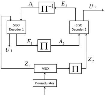
A turbo decoder is presented in Fig. 1.5. The two decoders are soft-in/soft out (SISO) decoders, which are matched to the encoders in Fig. 1.4 [10]. The left SISO decoder (D1) receives noisy data and parity bits from the channel, corresponding to the bits u(k) _and

u(1) _{generated by the upper convolutional encoder E1, performs the BCJR algorithm, and}

produces the bit-wise log likelihood ratios (LLRs) for the data bits and parity bits. The extrinsic information on the systematic bits E1 = U1 − A1 − Z1 is passed through the

interleaver to become the a priori input A2 of the second decoder D2. The second decoder

takes the permuted channel observationZ2 on the systematic bitsu(k) and respective parity

bits u(1) and feeds back extrinsic informationE2 which becomes the a priori information A1

(20)

Xingyu Xiang Chapter 1. Introduction 8 2

U

1 



E

2 1

A

SISO SISO SISO Decoder 1 SISO Decoder 2

E

A



1

E

A

2 1

U

1

Z

1

Z

2 MUX



Demodulator

Figure 1.5: Structure of turbo decoder

it is updated during each iteration. The two decoders work in an iterative manner until they meet a stopping criteria.

1.3.3

Linear Block Codes

Assume that the transmitted message, or information sequence is a bit stream from the binary field GF(2), i.e., only contains binary digits 0 and 1. Assume that the binary information sequence is divided into message blocks of fixed length k. The encoding process can be simply described by appending redundant bits to the current information bits. Then, the input messageb is transformed into a binary bit sequenceu with lengthn, wheren > k,

u is referred to as the codeword of the message b. The bits appended to each message block have length n−k; they contain no new information and just provide the capability of detecting and correcting transmission errors caused by the channel. Generating redundant bits with good error-correcting capability is a major concern in designing the channel codes. There may exist k linearly independent codewords, g0, g1, . . ., gk−1 such that every

codeword u is a linear combination of these k linearly independent codewords. If every codeword can be described as a linear combination of the k independent codewords, then it

(21)

Xingyu Xiang Chapter 1. Introduction 9 Let each of these linearly independent codewords represent one row of a matrix. The size

(k×n) matrix is called the generator matrix G and the encoding process can be expressed

as the matrix multiplication of message b and G; i.e., u = b·G. An (n, k) linear block code has more than one such basis and the generator matrix is not unique. The systematic form of a generator matrix is G = (Ik,P), where Ik is a (k ×k) identity matrix and P is

a k×(n−k) matrix. The linear block code generated by the generator matrix with this

form is referred to as a linear systematic code, which can be divided into two parts, the k unchanged information bits and the (n−k) parity-check bits. This can be also shown by the expression u =bG with the form (b,bP), the first k components of u are the same as the information sequence b.

The dual code B⊥ _{of linear code} _B _{is defined as:}

B⊥={x:b·xT = 0,∀b ∈ B}={x:G·xT = 0} (1.1)

The parity check matrix H of a linear block code B is the generator matrix of its dual code

B⊥_{. As such, a codeword} _b _{is in} _B _{if and only if the matrix-vector product} _HT_b _{= 0.}

The rows of matrix Hconsists of (n−k) linearly independent codewords fromB⊥ _{and each}

linearly independent codeword corresponds to a parity-check equation. A valid codeword should satisfy all parity-check equations. Since G has the dimension k byn, the dimension of His (n−k)×n when it is full rank. More coverage of linear block codes could be found in [7, 11].

1.3.4

Low-Density Parity-Check (LDPC) Codes

Low-density parity-check (LDPC) codes are a class of linear block codes with imple-mentable decoders, which provide near-capacity performance on a large set of transmission channels [12, 4]. As its name indicates, the parity-check matrix of LDPC code is “sparse”; i.e, it contains only a small number of nonzero entries. The sparseness ofH limits the decoding complexity when code length is increasing.

Except for the sparseness of the parity check matrixH, an LDPC code itself is no different from other block codes. It can be represented as (n, k), where n, k stand for the length of the codewordu and information bitsb, respectively. The corresponding full-rank Hhas the

(22)

Xingyu Xiang Chapter 1. Introduction 10 same dimension of (n−k)×nas that mentioned above. LDPC codes are decoded iteratively based on the structure of the parity-check matrix, so the construction of H is the major concern when designing LDPC codes with near-capacity performance.

The number of 1’s in a column of parity-check matrixHis called itscolumn weight, which is denoted by dv,i as the column weight of the ith-column. Therow weight is the number of

1’s in a row anddc,i is defined as the row weight of theith-row. When each column and each

row of matrix H has the same weight, i.e., dv,i and dc,i have unique value for all columns

and rows, the corresponding LDPC codes can be referred as (dv, dc) regular codes. On the

opposite side, irregular LDPC codes have different values of column weight or row weight, which are specified by the degree distributions described below.

The construction method for LDPC codes proposed by Mackay and Neal is to add ones to satisfy the column weight constraintdv. The location of the 1 entries are chosen randomly

from the rows which have less than the dc ones [4]. If there are rows with more positions

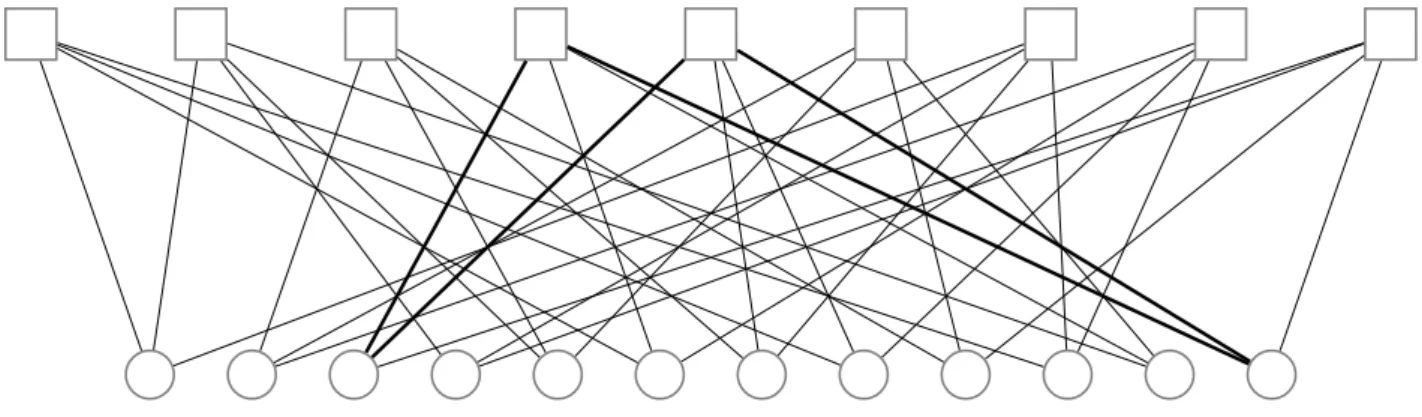
unfilled and there are columns remaining to be added, choose the entry position randomly so that the row and column weight are equal or less than designated. The process can be started again or backtracked by a few columns until the correct row weight distribution is satisfied. An example of a length-12 regular MacKay Neal parity-check matrix with weight distribution (dv = 3, dc = 4) is: H1 =                      1 1 1 1 1 1 1 1 1 1 1 1 1 1 1 1 1 1 1 1 1 1 1 1 1 1 1 1 1 1 1 1 1 1 1 1                      (1.2)

(23)

Xingyu Xiang Chapter 1. Introduction 11

Graphical representation of LDPC codes

After several decades of ignorance since LDPC codes had been invented by Gallager, an important breakthrough in the research of LDPC codes is that Tanner [13] used a bipartite graph to provide a graphical representation of the parity-check matrix. A bipartite graph is a graph in which nodes can be partitioned into two subsets such that there are no edges connecting nodes within the same subset. For the parity-check matrix of an LDPC code, the two subsets are referred to asvariable nodes andcheck nodes: n vertices for the variable nodes (or bit nodes), m vertices (m =n−k) for the check nodes. Each row of the parity-check matrix corresponds to one parity-check node and each column corresponds to one variable node. It follows that check-node iis connected to variable-nodej if the element (i, j) of the

H matrix is equal to 1, i.e., hij = 1. The Tanner graph corresponding to the parity-check

matrixHdenoted by (1.2) is shown in Figure 1.6. In the graph, the number of edges incident upon a node is called the degree of the node, so a bipartite graph of a (dv, dc) LDPC code

contains n variable nodes of degree dv and m check nodes of degree dc.

Figure 1.6: Tanner Graph corresponding to H1, the squares represent check nodes and the

circles represent check nodes.

Acycle in a Tanner graph is a sequence of connected vertices which start and end at the

same vertex in the graph and contain other vertices no more than once. The length of a cycle is the number of edges it contains. A bipartite graph only contains even-length cycles and the minimum length of a cycle contained in the graph is called the girth, which determines the performance of LDPC codes to some extent.

(24)

Xingyu Xiang Chapter 1. Introduction 12 properties of Tanner graph to generate some useful conclusions. The LDPC decoding can also be performed by using Tanner graph. After the major parameters of the Tanner graph are decided, which include the degrees of the variable and check nodes and the girth of the graph, we can still choose how the vertices of the graph are connected with each other.

Irregular LDPC code have different weight distribution in the columns or in the rows, thus they cannot be defined solely in terms of the weight (degree) parametersdv anddc [14].

We can instead use degree distributions ornode distributions to describe the variety of node degrees in the Tanner graph. A degree distribution can be described by a polynomial with the form:

γ(x) =X

i≥2

γixi−1, (1.3)

where γ(x) has nonnegative coefficients and γ(1) = 1. The use of polynomials leads to elegant and compact descriptions of the future results. γi denotes the fraction of edges in

the graph which are connected to a node of degree i. Thus an irregular code ensemble with length n can be fully described by degree distributionλ and ρ:

λ(x) =

dv

X

i≥2

λixi−1

where λ(x) specifies the variable-node degree distribution, which is the fraction of edges connected to variable nodes of degree i. Similarly, the check node degree distribution could be written as, ρ(x) = dc X i≥2 ρixi−1

whereρ(x) is the check-node degree distribution, which is the fraction of edges connected to check nodes of degree i. Regular (dv, dc) codes can also be represented by polynomials; e.g,

for the (3,6) regular code, we haveλ(x) = x2 _and _{ρ(x) =}_x5_.

Letn be the number of variable nodes and m be the number of check nodes. The check-node and variable-check-node degree distributions are related by the following set of equations:

m· Z 1 0 λ(x)dx=n· Z 1 0 ρ(x)dx (1.4)

(25)

Xingyu Xiang Chapter 1. Introduction 13 r(λ, ρ) = n−m n = 1− R1 0 ρ(x)dx R1 0 λ(x)dx , (1.5)

wherer is the LDPC code rate depending on the degree distribution. Equation (1.5) is valid when all the check equations are linearly independent, in other words, the corresponding parity-check matrix is full rank. We can also define node-perspective degree distribution as:

Λ(x) = dv X i≥1 Λixi P(x) = dc X i≥1 Pixi

where Λi is the fraction of variable nodes of degree i and Pi is the fraction of check nodes

of degreei. We can easily deduce the relationship between the edge degree distribution and node degree distribution as:

Λi = λi/i R1 0 λ(x)dx = Pλi/i j≥2λj/j Pi = ρi/i R1 0 ρ(x)dx = _Pρi/i j≥2ρj/j Decoding Algorithm

LDPC codes can be decoded using an iterative decoding algorithm whose complexity grows linearly with the length of the code. Codewordu is transmitted over the channel with the disturbing noise, and then the decoder will recover the information bits according to the received codeword. The sum-product decoding algorithm is a soft decision message-passing algorithm, which accepts the probability of each received bit as input [15]. The Tanner graph could be used to help understand the iterative decoding process, which could be treated as an exchange of messages between variable nodes and check nodes through the connected edges.

The input probabilities are called a priori probabilities for the received bits; the output probabilities of the decoder are called a posteriori probabilities because they are the condi-tional probability of the transmitted bits given the received bit probability or related evi-dence. In the sum-product message-passing decoding algorithm, all messages are assumed to

(26)

Xingyu Xiang Chapter 1. Introduction 14 be loglikelihood ratios (LLR), i.e., of the formL(ui) =log(p(0)/p(1)). Ifp(ui = 0)> p(ui = 1)

thenL(ui) is positive and the greater the magnitude the more possible thatui = 0. The

ben-efit of using logarithmic ratios is that they can transform the multiplication of probabilities into additions, which can clearly reduce implementation complexity.

The decoding process is to compute the maximum a posteriori probability for each code-word bit, Pi = P(ui = 1|N), which is the probability that the i-th codeword bit is a 1

conditioned on the eventN that all parity-check constraints are satisfied. Belief propagation on a graph without cycles can be closely approximated by the MAP algorithm.

Extrinsic information is the message sent from a node n along an edge e and cannot depend on any message previously received on edgee. The notation M(i) is the set of check nodes connected to variable node i, i.e., the positions of 1s in then-th column ofH. The set

N(j) contains variable nodes that participate in the the m-th parity-check equation, i.e., the positions of 1s in them-th row of H. LetN(j)\irepresents exclusion ofifrom the setN(j). The message from variable node ito check nodej is denoted as Zi→j, which is based on the

messages from all the check nodes connecting to variable nodeiexcept the check nodejitself. Another notation Zi is the a posteriori message of variable node i, which can be used for

the hard decision. Similarly, Lj→i denotes the message from thej-th check node to the i-th

symbol node based on all the variables checked by j excepti. y= [y1, y2, . . . , yn] denote the

received codeword. Omitting the proof, the iterative sum-product message-passing decoding algorithm [16] is listed as follows:

Step 1: Initialize Z_i(0) of each variable node i based on a posteriori LLR received from the channel. In the case of additive white Gaussian noise (AWGN) channel, Z_i(0) = _σ22yi for each variable node, where the σ2 is the variance for the additive noise.

Step 2: Variable nodes send Zi→j to each check nodej ∈ M(i).

Step 3: Check nodes connected to variable node i send

L(_jl_→)_i = 2tanh−1   Y i0∈N(j)/i tanh   Z(l−1) ji0 2     (1.6)

(27)

Xingyu Xiang Chapter 1. Introduction 15 own decision message Z_i(l) at the l-th iteration:

Z_i(_→l)_j = X j0∈M(i)/j L(l) j0i+L (0) n (1.7) Z_i(l)= X j∈M(i) L(_jil)+L(0)_n (1.8)

Step (2) and step (4) are repeated until the end of the decoding. The decoding process could be stopped early if the correct codeword is found or a preset maximum number of iterations is achieved.

1.4

Satellite Communication

Satellite communication plays a vital role in the global telecommunications by using ar-tificial satellites to provide communication links between various points on Earth. There are approximately 2000 artificial satellites orbiting Earth and they are responsible for relay-ing signals carryrelay-ing voice, video and data to and from one or multiple locations worldwide. Satellite communications can complement existing terrestrial infrastructure, providing com-petitive advantages such as greater coverage area, terrestrial-free network and the higher bandwidth. The limited access points also make satellite communications secure and private. But the high cost of launching satellites and the propagation delay are also the disadvantages for the satellites communication.

The two main components of satellite communication are the satellite itself, known as

the space segment and the ground segment, which consists of fixed or mobile transmission,

reception and ancillary equipments. The primary task of a satellite is to receive signals from a ground station and retransmit them down back to earth at a differen frequency. Some satellites also have the capability to process the received data before the retransmission. The data could be recovered first and then modulated using a different frequency or at a different data rate. The uplink indicates the process of an earth station transmits the signal up to the satellite. The terrestrial data may need to pass a baseband processor, a up converter, a high powered amplifier and through a parabolic dish antenna up to the

(28)

Xingyu Xiang Chapter 1. Introduction 16 designated satellite. The retransmission from the satellite to the ground station is termed

the downlink which works in the reverse fashion as the uplink.

The satellites could be categorized according to their service types; the fixed service satellites are responsible for the point to point communication, the broadcast service satellites are used for the satellite television or radio, the mobile service satellites are mainly for the satellite phone service. Different satellites use different frequency bands. The Ku band,

which ranges from 12-18 GHz, is used for fixed and broadcast services. The frequency range from 26.5 to 40 GHz Ka band is used for point to point communications.

1.4.1

DVB-S2 Standard

Digital Video Broadcasting (DVB) is a suite of internationally accepted open standards for digital television and radio broadcasting. The family of DVB standards are maintained by a Joint Technical Committee (JTC) of European Telecommunications Standards Institute (ETSI), European Committee for Electrotechnical Standardization (CENELEC) and Euro-pean Broadcasting Union (EBU). DVB systems distribute data using a variety of approaches, including:

• Satellite: DVB-S, DVB-S2 and DVB-SH

• Cable: DVB-C, DVB-C2

• Terrestrial television: DVB-T, DVB-T2

• Microwave: DVB-MT, DVB-MC and DVB-MS

These standards define the physical layer and data link layer and the main difference among them are the modulation schemes and error correcting codes. For the standards used for the same purpose, the second generation standard normally outperforms the previous gen-eration one by using adaptive modulation, more powerful channel coding and other advanced strategies. For instance, DVB-T is the first generation DVB standard for the transmission of digital terrestrial television. The second generation DVB-T2 adds the 256-QAM modulation and upgrades the error correct code from the combination of convolutional coding and Reed

(29)

Xingyu Xiang Chapter 1. Introduction 17 Solomon code to the combination of BCH and LDPC code. The same evolving trend can also be found from the DVB-S2 and DVB-C2.

Digital Video Broadcasting - Satellite (DVB-S) is the original DVB standard for the transmission of satellite television and dates. Its applications include the services in direct broadcast satellite like the Dish Network in the U.S. and Bell TV in Canada. Digital Video Broadcasting - Satellite - Second Generation (DVB-S2) is a digital television broadcast stan-dard that has been designed as a successor for the previous popular DVB-S system. It was developed in 2003 by the DVB Project. The standard is based on, and improves upon DVB-S by incorporating new coding and modulation schemes. The adaptive coding and modula-tion mode also make better use of the bandwidth under different transmission condimodula-tions. DVB-S2 is designed for broadcast services including standard and HDTV (High-definition television) signals, interactive services, and professional data content distribution. A better performance of about 30% gain is achieved by DVB-S2 than the previous DVB-S standard at the same transmission bandwidth and signal power.

1.4.2

APSK

Amplitude Phase Shift Keying (APSK) modulation transmits a data sequence by chang-ing both the amplitude and the phase of the carrier signal. It can be considered as a combination of phase-shift keying and amplitude-shift keying (ASK). It normally arranges the symbols into two or more concentric rings with a constant phase offset θ. For example, 16-APSK uses a double ring PSK format, this is called 4−12 16-APSK with four symbols in the center ring and 12 in the outer ring, which is shown in Fig. 1.7.

APSK is an attractive modulation scheme for nonlinear satellite channels due to its power and spectral efficiency together with the robustness against nonlinear distortion. The concept of APSK modulation and its suitability for nonlinear channels was proposed in [17]. At that time, it was concluded that PSK performs better than APSK modulation over nonlinear channel with single carrier operation. However, based on the results from [18], this conclusion was reverted and APSK became a popular modulation scheme for advanced satellite communications. The commercial applications of APSK include DVB-S2, DVB-SH

(30)

Moreover their performance on linear channels are almost as good as their QAM competitors.

(a) QPSK (b) 8-PSK

(c) 16-APSK (d) 32-APSK Figure 6. Constellation Labelings

00 I Q ρ=1 ρ=1ρ=1 ρ=1 10 11 ₀₁ 000 I Q ρ=1 ρ=1 ρ=1 ρ=1 011 111 001 101 010 110 100 text 1100 1101 1111 1110 0000 0100 0101 0001 1001 1011 0011 0111 0110 0010 1010 1000 I Q R1 R2 text 10001 10011 10111 10101 00000 10000 10010 00010 00011 00111 00110 10110 10100 00100 00101 00001 I Q R1 R2 R3 11000 01000 11001 01001 01101 11101 01100 11100 11110 01110 11111 01111 01011 11011 01010 11010 Figure 1.7: 16-APSK

(Digital Video Broadcasting via Satellite to Handheld devices) and IPoS (Internet Protocol over Satellite), etc.

1.4.3

TWTA

A traveling-wave tube (TWT) is a specialized vacuum tube that is used to provide power amplification for signals with high frequency. It is usually integrated as part of an assembly known as a traveling-wave tube amplifier (TWTA), which is normally used as the amplifier in satellite transmitter. TWTAs provide high power amplification for the input weak signals, while it also cause side effects along with their efficient amplification performance.

There are several aspects to specify the characteristics of a TWTA:

• Peak Power

• AM/AM Transfer and AM/PM Conversion curves

• Input Back-off (IBO) vs. Output back-off (OBO)

• Gain

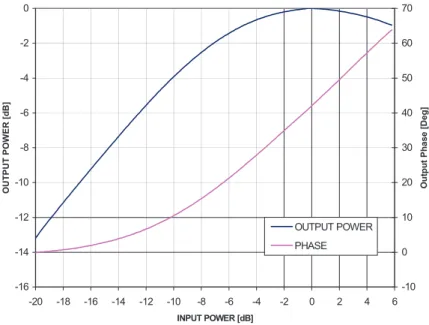
The curves of output power as the function of the input power for TWTAs are also called AM/AM transfer curves. The blue curve in Fig. 1.8 shows the AM/AM transfer

(31)

ETSI

ETSI EN 302 307 V1.2.1 (2009-08) 73

Figures H.11 and H.12 give the AM/AM and AM/PM TWTA characteristics. Ku-band LTWTA Single Carrier Transfer Characteristics

(Measurement Frequency: 10992.5MHz) -26 -24 -22 -20 -18 -16 -14 -12 -10 -8 -6 -4 -2 0 -30 -28 -26 -24 -22 -20 -18 -16 -14 -12 -10 -8 -6 -4 -2 0 2 4 6 Pin (dB) Pout ( d B ) 0 5 10 15 20 25 30 Output P h

ase Change (Deg)

Figure H.11: Linearized TWTA characteristic

Ka-band TWTA - Single Carrier Transfer Characteristics

-16 -14 -12 -10 -8 -6 -4 -2 0 -20 -18 -16 -14 -12 -10 -8 -6 -4 -2 0 2 4 6 INPUT POWER [dB] O U T P UT P O WE R [d B] -10 0 10 20 30 40 50 60 70 Ou tp u t P h a se [D eg ] OUTPUT POWER PHASE

Figure H.12: Non-Linearized TWTA characteristic Figure 1.8: Non-Linearized TWTA characteristic1

characteristic of aKa band (frequency range from 26.5-40 GHz) TWTA defined in DVB-S2

standard [19]. The output increase as the increasing of input power until the input power reaches certain region. At a point called saturation, any further increase in input power produces no further increase in output power. The saturate point or region is designed at input power level of 0 dBm for most TWTAs. Channel amplifiers are often used before the TWTA to assure the input power level is either near the saturation or at some other pre-determined input power values.

The power level that the TWTA is actually being operated is called the operating point

or back-off. The operating point of the input power is called Input Back-off (IBO), and

Output Back-off (OBO) means the corresponding output power value. Generally the OBO

attracts more attention in the satellite operation terms since the operator is more concerned about the total power generated out of the transponder. Theoretically the TWTA should be operated at the saturation point to achieve the maximum output power, but the non-linear behavior when operating around the saturation point or the near region causes significant signal distortions. So the real operation point is determined individually under different circumstances.

(32)

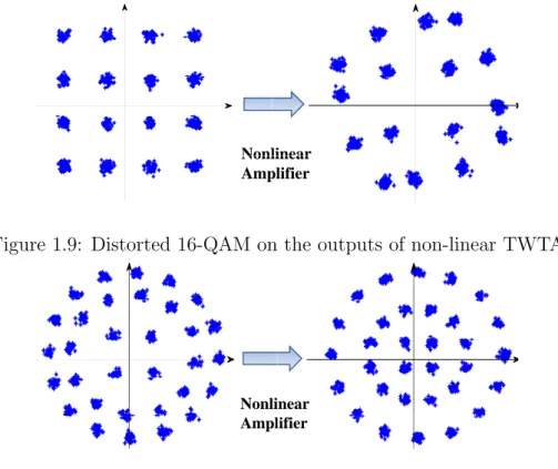
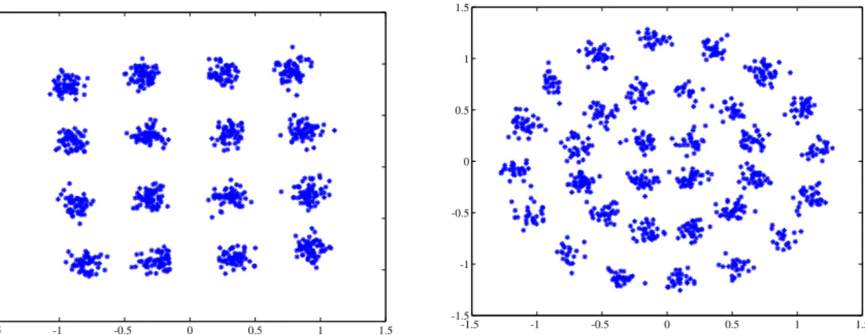
Xingyu Xiang Chapter 1. Introduction 20 Nonl Nonl Amp linear linear plifier

Figure 1.9: Distorted 16-QAM on the outputs of non-linear TWTA

Nonli Ampl

inear lifier

Figure 1.10: Distorted 32-APSK on the outputs of non-linear TWTA

Aside from the amplitude transfer curves, phase shift properties are also a key character-istic provided by the TWTA manufacturers. The phase shift is another cause of degradation because of the non-linearity of the amplitude. The phase distortion depends on the drive level, i.e., the input power level. The curve of the phase shift versus the input back off is shown as a pink curve in Fig. 1.8. The two characteristic curves in that figure are all for K −a band TWTA for the DVB-S2 standard. The original figure could be found in the appendix of [19]. The phase shift curve can be called the AM/PM conversion curve. The degradation of the phase shift is about 0.6 dB and the non-linear amplitude could effect up to 2.5 dB of the signal to noise ratio [20].

To better understand the impact of nonlinear characteristic of TWTA, two examples corresponding to 16-QAM and 32-APSK are shown in Fig. 1.9 and 1.10. The sub-figures in the left show the constellation symbols with additive noise. The noise variance is set to be low to keep the constellation recognizable. The sub-figures in the right are the distorted symbols through non-linear TWTA, which shows both the amplitude and phase impact generated by the TWTA. From these two figures, APSK symbols preserve a good shape while the positions

(33)

Xingyu Xiang Chapter 1. Introduction 21 Pre-distortion IBO, dB OBO, dB TWTA, AM/AM IBO, dB IBO, dB

Figure 1.11: Magnitude Predistortion linearizers generate a response opposite to a TWTA’s characteristics Phase Pre-distortion IBO, dB Phase Rotation TWTA, AM/PM IBO, dB IBO, dB ϕ

Figure 1.12: Phase Predistortion linearizers generate a response opposite to a TWTA’s characteristics

of QAM symbols are significantly changed under the non-linear distortion. Except adopting modulations schemes like APSK, the amplifier non-linearity impairment can be reduced by using a technique called pre-distortion.

Pre-distortion is one of the strategies to compensate the nonlinearities of the amplifier. The principle of pre-distortion is to distort the signals before transmitting to the amplifier, the distortion operation is achieved by an additional device whose characteristics are close to the inverse of those of the amplifier. The detail about the linearizing of high power amplifier could be found in [21, 22, 23, 24, 25].

A typical amplitude transfer characteristic of the TWTA is shown in the middle part of Fig. 1.11, the sum of the characteristic from the predistorter and the TWTA would cancel out the non-linearity of the TWTA and the resulted linear AM/AM transfer curve is shown in the rightmost figure. The same operation to mitigate the phase distortion caused by the TWTA can also be achieved by the pre-distortion 1.12. The predistorter, or the linearizer, has to match the characteristics of the TWTA in order to produce the maximum beneficial effects. The algorithms to implement the pre-distortion strategy can be found in [26, 27]. Fig. 1.13 shows the linearized constellation symbols of 16-QAM and 32-APSK after passing through the predistortion followed by the TWTA.

(34)

Xingyu Xiang Chapter 1. Introduction 22 -1.5 -1 -0.5 0 0.5 1 1.5 -1.5 -1 -0.5 0 0.5 1 1.5 -1.5 -1 -0.5 0 0.5 1 1.5 -1.5 -1 -0.5 0 0.5 1 1.5

Figure 1.13: Predistorted QAM and 32-APSK on the outputs of non-linear TWTA

The benefits of a linearized TWTA are obvious: the linear region can be expanded and cause smaller non-linear effects. The disadvantages include the requirement of additional power and the additional weight of the extra equipment, the difficulty of tuning and not suitable for all traffic types.

1.4.4

DVB-S2 Performance

The original standard DVB-S uses QPSK modulation with concatenated convolutional and Reed-Solomon codes. The evolved DVB-S2 chose the enhanced modulation schemes and low density parity check (LDPC) codes which actually provided more than 35% throughput improvement with respect to the previous DVB-S standard. For the LDPC codes defined in DVB-S2 standard, certain structure is imposed on parity check matrices to facilitate the codes description and easy encoding. More specifically, the parity check matrix H is restricted to be the following form:

H(N−K)×N =

A(N−K)×KB(N−K)×(N−K)

(1.9) Where B is dual diagonal sub-matrix:

(35)

Xingyu Xiang Chapter 1. Introduction 23 Bn−k,n−k=                1 1 1

0

1 1 1

0

...

₁ 1 1                (1.10)

Then the parity bits can be solved recursively based on the speciality structure of the dual diagonal matrix. The code with such structure parity-check matrix is also known as an

extended irregular repeat accumulate (eIRA) code [28].

9.8 10.1 10.4 10.7 11 11.3 11.6 11.9 12.2 12.5 12.8 13.1 13.4 13.7 10-5 10-4 10-3 10-2 10-1 E s/N0 in dB BER 32APSK R=4 (R c=0.8) 32APSK R=3.75 (R c=0.75) 16APSK R=3.2 (R c=0.8) 32APSK R=3 (R c=0.6) 16APSK R=3 (R c=0.75)

Figure 1.14: Performance of DVB-S2 standardized LDPC coded over AWGN channel In DVB-S2, a wide range of bandwidth efficiencies from 0.5 bits per symbol up to 4.5 bits per symbol is covered by defining ten different code rates 1/4,1/3,1/2,3/5,2/3,3/4,4/5,5/6,8/9 and 9/10 with four different modulation schemes QPSK, 8-PSK, 16-APSK, 32-APSK. The error performances of the uncoded modulation schemes are shown in Fig. 1.2. 32-APSK has the worst error performance while it could transmit the most number of bits per symbol. The LDPC coded block length can be eitherN = 16 200 (short) orN = 64 800 (normal) bits

(36)

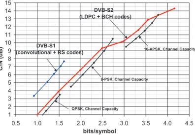
Xingyu Xiang Chapter 1. Introduction 24 important to note that the DVB-S2 design follows closely the theoretical limit for the

entire range of operation. Also compared to DVB-S concatenated convolutional and Reed-Solomon codes, a capacity improvement of more than 35% is achieved at the same C/N.

Figure 13. Comparison of DVB-S2 (LDPC+BCH) Codes to DVB-S1 and Channel Capacity

6 Conclusion:

LDPC codes of DVB-S2 approach Shannon limit to within 0.6-0.8 dB for a wide range of throughput and yet they are easy to implement. It may be hard to justify their

replacements for decades to come. References:

1. R. G. Gallager, “Low density parity check codes”, IRE Trans. Info. Theory, 1962, IT-8, pp. 21-28

2. D. J. MacKay and R. M. Neal, “Good codes based on very sparse matrices”, 5th_IMA Conf. 1995, pp.100-111

3. D. J. MacKay and R. M. Neal, “Near Shannon limit performance of low density parity check codes”,

Electronics Lett. Mar. 1997, vol. 33, no.6, pp. 457-458

1 2 3 4 5 6 7 8 9 10 11 12 13 14 15 0.5 1.0 1.5 2.0 2.5 3.0 3.5 4.0 4.5 bits/symbol C/N ( d B) DVB-S2 (LDPC + BCH codes) 8-PSK, Channel Capacity QPSK, Channel Capacity DVB-S1

(convolutional + RS codes) 16-APSK, Channel Capacity

Figure 1.15: Comparison of DVB-S2 Codes to DVB-S and Channel Capacity2

for all rates. To improve the performance, irregular LDPC codes are used where degrees of variable nodes are different.

Performance of various code rates with 16-APSK and 32-APSK constellations on AWGN channel is depicted in Figure 1.14. Maximum number of decoder iterations is set to be 100. If no valid codeword is found then the current decoder outputs are estimated at the end of 100-th iterations.

For comparison, the performance of DVB-S code and Shannon limits of constellations are provided in [19] and cited as Fig. 1.15. It is important to note that the system operation parameters of DVB-S2 are chosen by following the theoretical limit. Compared to the con-catenated convolutional and Reed-Solomon codes in DVB-S, the improvement of more than 35% is achieved by using the modern channel coding strategy [29].

1.5

Thesis Outline

The objective of the dissertation is to improve the performance of systems like DVB-S2 that use APSK modulation and LDPC coding. Several strategies including constellation shaping, LDPC coding optimization, modulation optimization are used to push the system to approach the theoretical limit.

(37)

Xingyu Xiang Chapter 1. Introduction 25 The dissertation is divided into 5 chapters. Chapter 2 covers the channel capacity con-cepts and the idea of constellation shaping. Chapter 3 introduces the shaping system with 16-PAM and 32-APSK modulation Both turbo codes and LDPC codes are used as the chan-nel coding scheme to test the constellation strategy. A useful tool named EXIT charts is reviewed in Chapter 4 and used to optimized the degree distribution of LDPC codes. Con-stellation symbol mapping are investigated to find better rules than the DVB-S2 standard. Bit error rate results indicate the performance improvement by combining better mapping rules with optimized LDPC codes.

(38)

26

Chapter 2

Channel Capacity and Constellation

Shaping

In a digital communication system, reliable transmission requires that the useful source signal be reconstructed at the sink with an arbitrarily low probability of error. The maximum transmission rate at which reliable transmission can be satisfied is called thechannel capacity [30]. This chapter begins with a discussion of the concept of capacity. A numerical method for calculating capacity value is presented and compared with results generated by

Monte-Carlo simulation. In addition, a simple method to change the input symbol distribution

calledconstellation shaping is introduced as a strategy to better approach the capacity limit under modulation constraint. Next, the system model including constellation shaping, i.e.,

shaped system is described. Several examples are given to help understand the shaping

strategies. The optimized parameters for shaped systems with PAM and APSK modulation are found based on mutual information analysis. Thepeak to average power ratio for shaped system is also considered and the summary is given at the end of this chapter.

2.1

Channel Capacity

As the upper bound on the amount of reliably transmitted information, channel capacity can also be interpreted as a theoretical criteria that should be maximized given the system constraints such as modulation types, channel conditions etc. Channels with additive white

(39)

Xingyu Xiang Chapter 2. Channel Capacity and Constellation Shaping 27 gaussian noise (AWGN) are the main focus of this chapter. The derivation of channel capacity is reviewed in the beginning of this section, then Monte-Carlo simulation and

Gaussian-Hermite quadrature are introduced as methods for calculating the capacity. Several capacity

examples are given after introducing two coded modulation system models, which are called

bit-interleaved coded modulation (BICM) and bit-interleaved coded modulation with iterative

decoding (BICM-ID) system.

2.1.1

The Unconstrained Capacity

Thediscrete channel is a system consisting of an input alphabetX, an output alphabetY

and a probability transition probability for each pair of input symbol xi and output symbol

yi. The transition probability p(yi|xi) is the conditional probability of receiving output

symbol yi given that xi is transmitted. Only memoryless channels are considered in this

dissertation, in which the output probability distribution only depends on the channel input at the same time. The model for a discrete-time AWGN channel is,

yi =xi+zi, (2.1)

where yi is the channel output at time i. The output of the channel is the summation

of the channel input and additive Gaussian noise. The input signal xi is assumed to be

independent of noise zi, which is Gaussian distributed with zero mean and varianceN. The

mutual information I(X;Y) can be expanded as:

I(X;Y) = H(Y)−H(Y|X)

= H(Y)−H((X+Z)|X) = H(Y)−H(Z|X)

= H(Y)−H(Z). (2.2)

The channel capacity is defined as the maximum value of mutual information between the channel input and output over all possible input distributionp(X). The input of the channel is normally power limited, otherwise it may lead to infinite channel capacity. The capacity

(40)

Xingyu Xiang Chapter 2. Channel Capacity and Constellation Shaping 28 of Gaussian channel with power constraint P is:

C = max

p(x), E(X2₎_≤_PI(X;Y), (2.3) Since Z is Gaussian distributed noise and independent of X, the entropy of which is

H(Z) = 1₂log 2πeN according to the entropy definition [1]. The entropy of the output Y is

bounded by 1₂log 2πe(P +N) based on the theorem that the normal distribution with given variance maximized the entropy. The notationP is the power constraint of the channel input X and N is the noise variance [1]. Equation (2.2) can be written as:

I(X;Y)≤ 1 2log 2πe(P +N)− 1 2log 2πeN = 1 2log 1 + P N (2.4) The maximum mutual information I(X;Y) is achieved whenY is Gaussian distributed, the input X should be also Gaussian since the noise follows Gaussian distribution. The units of capacity in the form of equation (2.4) is bits per transmission or bits per channel use. Channel capacity is the upper bound on the transmission rate for reliable communication over the noisy channel. If the bit transmission rate is greater than capacity C, it is not possible to recover the information bits with arbitrary small error probability.

The channel with waveform inputs and outputs is also calledcontinuous time channel or

waveform channel with model of Y(t) =X(t) +Z(t). Assume that the channel has limited

bandwidthW and the channel noise is additive white Gaussian noise. This continuous-time AWGN channel can be reduced to an equivalent discrete-time AWGN channel according to the sampling theorem and the theorem of irrelevance [1]. The continuous input and output signal could be represented by discrete samples spaced by Nyquist’s sampling rate. The continuous-time signal with bandwidth W during time interval [0, T] can be completely determined by 2W T samples. The signal power per sample is P/2W and the noise power per sample is N0/2, where N0 is the noise power per unit of bandwidth. It follows that the

channel capacity per sample can be written as:

C = 1 2log 1 + P 2W N0 2 ! = 1 2log 1 + P N0W

. bits per sample (2.5)

(41)

Xingyu Xiang Chapter 2. Channel Capacity and Constellation Shaping 29 per second: C =Wlog 1 + P N0W

. bits per second (2.6)

The capacity can be more informative when described as the function of bit energy Eb

C = Wlog 1 + P N0W (2.7) = Wlog 1 + Ebrb N0W bits/sec. (2.8)

where rb is the data rate. There are several interesting results that can be obtained by

replacing rb with C and treatingC/W as the normalized channel capacity with units of bits

per second per Hz.

C W = log 1 + C W Eb N0

The signal to noise ratioEb/N0should increase exponentially to makeC/W approach infinity.

The minimum Eb/N0 is −1.6 dB as C/W getting close to 0.

Fading channels are characterized as having a random fluctuation in the received ampli-tude. For such channels, the concept of capacity can be extended to the so-called ergodic

capacity. Fading channels can be modeled as Yi = hi · Xi + Zi, where hi is the fading

coefficient. A simple fading model is ergodic Rayleigh fading channel, in which the fading coefficient hi is independent and identically distributed (i.i.d.) Rayleigh distributed and the

channel information is known at the receiver for every time instant. Let ˆP denote the aver-age transmit signal power, N0/2 the noise power spectral density, and W the received signal

bandwidth. The instantaneous received SNR is then ˆP h[i]/N0B and its expected value is

ˆ

Pˆh/N0W. Since ˆP /N0W is a constant, the distribution of fading coefficientsh[i] determines

the distribution of SNR. To find the capacity, we must average over the distribution of h[i], i.e., C = E_|_h_[_i_]_|2 " Wlog₂ 1 + ˆ P|h[i]|2 N0W !# = Z ∞ −∞ Wlog₂ 1 + ˆ P x N0W ! p(x)dx = Z ∞ −∞ Wlog₂(1 +β)p(β)dβ (2.9)

(42)

Xingyu Xiang Chapter 2. Channel Capacity and Constellation Shaping 30 where β = _N