LOW-COST DEEP LEARNING UAV AND RASPBERRY PI SOLUTION TO REAL TIME PAVEMENT CONDITION ASSESSMENT
By
Murad Al Qurishee Weidong Wu
Assistant Professor of Civil Engineering (Committee Chair)
Joseph Owino
Professor of Civil Engineering and Department Head
(Committee Co-Chair) Ignatius Fomunung
Professor of Civil Engineering (Committee Member)
Mbakisya A. Onyango
Associate Professor of Civil Engineering (Committee Member)
Yu Liang
Associate Professor of Computer Science (Committee Member)
LOW-COST DEEP LEARNING UAV AND RASPBERRY PI SOLUTION TO REAL TIME PAVEMENT CONDITION ASSESSMENT
By
Murad Al Qurishee
A Thesis Submitted to the Faculty of the University of Tennessee at Chattanooga in Partial
Fulfillment of the Requirements of the Degree of Master of Science: Engineering The University of Tennessee at Chattanooga
Chattanooga, Tennessee May 2019
iii
Copyright © 2019 Murad Al Qurishee All Rights Reserved
ABSTRACT
In this thesis, a real-time and low-cost solution to the autonomous condition assessment of pavement is proposed using deep learning, Unmanned Aerial Vehicle (UAV) and Raspberry Pi tiny computer technologies, which makes roads maintenance and renovation management more efficient and cost effective. A comparison study was conducted to compare the
performance of seven different combinations of meta-architectures for pavement distress classification. It was observed that real-time object detection architecture SSD with MobileNet feature extractor is the best combination for real-time defect detection to be used by tiny
computers. A low-cost Raspberry Pi smart defect detector camera was configured using the trained SSD MobileNet v1, which can be deployed with UAV for real-time and remote pavement condition assessment. The preliminary results show that the smart pavement detector camera achieves an accuracy of 60% at 1.2 frames per second in raspberry pi and 96% at 13.8 frames per second in CPU-based computer.
DEDICATION
ACKNOWLEDGEMENTS
First and foremost, I would like to express my thanks to the Almighty Allah for providing me a golden opportunity and healthy life to pursue a master’s degree on Artificial Intelligence (AI) using UAV at the University of Tennessee at Chattanooga (UTC), my deepest appreciation and humbleness to Him. Thanks to my parents, my beautiful wife, my lovely son, and my family members to support me to pursue master’s degree without any delay. They support me in
mentally as well as financially to go through the educational system of the USA.
I am also grateful to Allah to have Dr. Weidong Wu as my academic advisor and coordinator. Dr. Wu is a nice and easy access person with good knowledge of advanced technologies in civil engineering, and I am thankful to him for his supervision, support,
guidance, constructive criticism, and encouragement. Also, my gratitude is will go to Dr. Owino, Dr. Fomunung, Dr. Onoyango, and Dr. Liang for their intellectual support and critical criticism of my thesis manuscript. Moreover, my gratitude to Dr. Arash for his advice and good
recommendation to pursue my PhD study.
I would like to thank TN Board of Architectural and Engineering Examiners (TBAEE) and University of Tennessee at Chattanooga (UTC) for funding support. Supercomputer resources used for deep learning simulations provided by Drs Anthony Skjellum and Ethan Hereth and UTC SimCenter are greatly appreciated.
I would like to thankful to Mrs. Lemon, Mrs. Anderson, Mrs. Cook, and other staffs of the Department of Civil and Chemical Engineering for their support and encouragement of my study at UTC.
I thank my fellow lab-mate Mr. Babatunde Atolagbe for the encouragement, for the sleepless nights we worked together, and all the fun that we made during 2 years of long journey. Moreover, my special thanks to Mawazo Fortonatos, Abubakr Ziedan, Sayed Mohammad Tarek, Shuvasish Roy, Maxwell Omwenga, and Raiful Hasan for their support in on-campus or off-campus. Last but not the least, I would thankful to Dr. Richard Wilson; Clarence Francis to make my stay in the U.S. memorable and enjoyable. Their support cannot measure in terms of money.
TABLE OF CONTENTS ABSTRACT ... iv DEDICATION ... v ACKNOWLEDGEMENTS ... vi LIST OF TABLES ... x LIST OF FIGURES ... xi
LIST OF ABBREVIATIONS ... xiii
CHAPTER I. INTRODUCTION ... 1
1.1 Problem Statement ... 4
1.2 Objectives of the Study...4
1.3 Scope of the Study ... 5
1.4 Thesis Overview ... 5
II. LITERATURE REVIEW ... 6
2.1 Types of Pavement Damages ... 7
2.2 History of Deep Learning ... 14
2.3 Types of Deep Learning Architectures... 16
Unsupervised Pretrained Networks ... 16
Recurrent Neural Networks (RNN) ... 19
Recursive Neural Networks ... 20
Convolutional Neural Networks (CNNs)... 22
2.4 Application of Deep Learning Techniques in Civil Engineering ... 27
3.1 Datasets ... 34
Image Data Acquisition ... 34
Data Preprocessing... 34
3.2 Evaluation of the Four Real-Time Object Detection Networks... 36
Faster R-CNN ... 37 R-FCN ... 38 YOLO ... 38 SSD ... 39 3.3 Model Hyperparameters... 39 3.4 Computational Platform ... 41
IV. RESULTS AND DISCUSSION ... 42
4.1 Real-Time Video Test ... 43
4.2 Configuration of a Raspberry Pi Camera Module ... 49
4.3 Testing on Real-Time Video ... 53
4.4 Automatic 3D Drone Mapping Area Calculation ... 54
4.5 Location of the Crack... 56
V. CONCLUSION AND RECOMMENDATIONS... 58
REFERENCES ... 60
APPENDIX A. BOX CLASSIFIER CLASSIFICATION LOSS ... 69
B. TOTAL LOSS ... 73
C. GLOBAL STEPS ... 77
D. CLONE LOSS ... 80
LIST OF TABLES
Table 3.1 Model properties and hyperparameters ...40 Table 4.1 Comparison of models based on mAP and real-time speed ...44 Table 4.2 Cost of Raspberry Pi crack detector camera kit ...50
LIST OF FIGURES
Figure 2.1 Alligator cracking ...7
Figure 2.2 Block cracking ...8
Figure 2.3 Edge crack (ASTM, 2011) ...9
Figure 2.4 Pothole ...9
Figure 2.5 Longitudinal crack ...10
Figure 2.6 Transverse crack ...10
Figure 2.7 Patch and utility cut ...11
Figure 2.8 Rutting (ASTM, 2011) ...12
Figure 2.9 Shoving (ASTM, 2011) ...12
Figure 2.10 Weather and raveling (ASTM, 2011) ...13
Figure 2.11 Corner break (ASTM, 2011) ...13
Figure 2.12 Divided slab crack ...14
Figure 2.13 DBN model with stacks of pretrain RBM and feed-forward multilayer perceptron (Adam Gibson & Patterson, 2018) ...18
Figure 2.14 Unfolding typical forward computational RNN diagram ...20
Figure 2.15 Typical recursive neural network ...21
Figure 2.16 Typical ConvNet architecture ...23
Figure 2.17 Configuration of convolution operation in the feature extraction network ...24
Figure 2.18 Yielding of feature map after the implementation of stride and convolution kernel...25
Figure 3.1 Workflow of a UAV/deep learning/Raspberry Pi pavement defect detection
solution ...32
Figure 3.2 An outline of process and methodologies ...33
Figure 3.3 Configuration of the drone and the infrared thermal camera for data acquisition ...34
Figure 3.4 Sprite image of standard (1st to 8th rows) and thermal image (9th to 11th rows) data ...36
Figure 3.5 Faster-RCNN architecture ...38
Figure 4.1 Comparison of total loss of different models ...43
Figure 4.2 Pavement distress classification and localization using Faster R-CNN with Inception ...45
Figure 4.3 Pavement distress classification and localization using Faster R-CNN with NasNet...46
Figure 4.4 Pavement distress classification and localization using Faster R-CNN with ResNet101 ...46
Figure 4.5 Pavement distress classification and localization using R-FCN with Resnet101 ...47
Figure 4.6 Pavement distress classification and localization using SSD with MobileNet ...47
Figure 4.7 Pavement distress classification and localization using SSD with Inception...48
Figure 4.8 Pavement distress classification and localization using YOLO ...48
Figure 4.9 Pavement distress classification and localization using Faster R-CNN with on infrared image ...49
Figure 4.10 Raspberry Pi 3 B+ crack detector camera configuration ...51
Figure 4.11 Workflow of Raspberry Pi 3 B+ crack detector camera ...51
Figure 4.12 Raspberry Pi is attached with drone ...52
Figure 4.13 Drone with Raspberry Pi camera is in action to inspect the pavement defects ...53
Figure 4.14 Comparison of one minute real time speed of different models in GPU based computer ...54 Figure 4.15 One minute real-time speed of SSD Mobilenet V1 in Raspberry Pi
3 B+ ...54 Figure 4.16 Crack dimension determination using PIX4D software ...55 Figure 4.17 Coordinates of the crack found using Geotag software ...56 Figure 4.18 Google Earth view of crack using the GPS coordinate from the Geotag
LIST OF ABBREBIATIONS AC, Asphalt Concrete
AdaBoost, Adaptive Boosting AI, Artificial Intelligence
ASCE, American Society of Civil Engineers CIFAR, Canadian Institute For Advanced Research CNN, Convolution Neural Network
ConvNet, Convolution Neural Network DBN, Deep Belief Network
DCDR, Double-Center-Double-Radius EEG, Electroencephalography
FP, Flexible Pavement
GAN, Generative Adversarial Networks GPU, Graphical Processing Unit
HIS, Hue-Saturation-Intensity mAP, Mean Average Precision ML, Machine Learning
MLP, Multi-Perceptron Neural Network
MNIST, Modified National Institute of Standards and Technology NCHRP, National Cooperative Highway Research Program
NORB, NYU Object Recognition Benchmark RBM, Restricted Boltzmann Machines
ReLU, Rectified Linear Unit
R-FCN, Region Based Fully Convolution Networks RGB, Red-Green-Blue
RNN, Recurrent Neural Networks RP, Rigid Pavement
RPN, region proposal network SSD, Single Shot Multibox Detector UAV, Unmanned Aerial Vehicle YOLO, You Only Look Once
CHAPTER I INTRODUCTION
The US highways and roads are in poor condition due to aging, increasing traffic loads, and severe environmental hazards. The ASCE 2017 report card (ASCE, 2018) gives a score of D for roads (poor at risk condition) although overall US infrastructure earns D+ score (fair
condition). It was also reported that 21% or approximately one out of five of the US highways had poor pavement condition in 2015. According to 2017 Pavement Management System Report by the Tennessee Department of Transportation, the pavement smoothness index (PSI) of
Chattanooga Interstate and State Route is 3.32 and 3.76 respectively which indicates the good condition of pavement condition in Chattanooga (TDOT, 2019).
Purely manual survey, semi-automated or automated techniques have been used to assess pavement condition (Koch, Georgieva, Kasireddy, Akinci, & Fieguth, 2015; McGhee, 2004). Traditionally manual and visual assessment requires engineers working on busy roads, which can rather dangerous, costly, time-consuming and inefficient. The semi-automated method uses a downward looking video camera to collect images and videos, which are then analyzed by experienced engineers. The semi-automated method uses a downward looking video camera to collect images and videos, which are then analyzed by experienced engineers. This video can be collected either using camera or drone. However, after collecting this video or images, it takes enough time to analyze it manually.
Ground Penetrating Radar (GPR) (Evans, Frost, Stonecliffe-Jones, & Dixon, 2008; Wimsatt, Scullion, Ragsdale, & Servos, 1998) is another semi-automatic method that maps subsurface conditions of pavements and then use data analysis method to evaluate the condition of pavement. The drawback of GPR for pavement evaluation is the shortage of reliable
automated data analysis procedures, as well as the difficulty of manually interpreting the large amounts of GPR data (Evans et al., 2008). Both manual and semi-automatic methods rely on experienced experts.
Computer vision-based defect detection is a strong candidate for automated pavement condition assessment. In 2011, National Cooperative Highway Research Program (NCHRP) published a survey conducted on state-of-the-art techniques and technologies such as laser-based imaging automated systems for acquiring high-quality 2-D and 3-D pavement surface images (Wang & Smadi, 2011). Many researchers have contributed to the development of automatic robotic infrastructure health monitoring system using different computer vision based approaches such as edge detection, K-means clustering, image binarization, wavelet transformation, Canny algorithm, Roberts algorithm, Prewitt algorithm (Vincent & Folorunso, 2009), Laplacian algorithm (Parker, 2010), statistical approach (Sinha & Fieguth, 2006), pattern recognition, clustering, percolation model (Yamaguchi & Hashimoto, 2010), depth camera, and so on. However, most image processing techniques are limited to detect one specific type of damage from still image such as concrete cracks (Abdel-Qader, Abudayyeh, & Kelly, 2003), loosened bolts (Cha, Choi, & Büyüköztürk, 2017; Park, Kim, & Kim, 2015), concrete spalling (German, Brilakis, & DesRoches, 2012), asphalt pavement pothole detection (Jo & Ryu, 2015), and pavements cracks (Cord & Chambon, 2012; Ying & Salari, 2010; Zalama, Gómez‐García‐ Bermejo, Medina, & Llamas, 2014). Recently, researchers started using deep neural
networks-based defect detection techniques (Cha, Choi, & Büyüköztürk, 2017; Cha, Choi, Suh,
Mahmoudkhani, & Büyüköztürk, 2017; Gopalakrishnan, Khaitan, Choudhary, & Agrawal, 2017; Maeda, Sekimoto, & Seto, 2016; Makantasis, Protopapadakis, Doulamis, Doulamis, & Loupos, 2015; A. Zhang et al., 2017). Most of these proposed models focus only on detection and classification. Other information such as dimensions and locations of the pavement distress still miss, and they are critical to the determination of distress dimension, geometry, and ratings. Quantification of pavement distress will help pavement management and maintenance, thus lead to timely maintenance. Koch et.al. summarized computer vision methods for condition
assessment of different types of infrastructure including pavement, they concluded that
processing of image and video data is not yet fully automatic, challenges such as lack of robust algorithms, insufficient labeled images for training machine learning (ML) neural network, and lack of defect detection computer models that can handle realistic environmental conditions remain (Koch et al., 2015).
With the recent boom of Artificial Intelligence (AI)/deep learning computer technology and more affordable UAV available on the market, inspired by (Amato et al., 2017), a low-cost, real-time, efficient solution is proposed that facilitates UAVs, deep learning and the low-cost Raspberry Pi (Pi—Teach, 2018) tiny computer to pavement condition assessment. To
accommodate real-time object detection needs and reduce the computation burden of Raspberry, four end-to-end convolutional neural network (CNN) models (Liu et al., 2016; Redmon, Divvala, Girshick, & Farhadi, 2016; Redmon & Farhadi, 2017; Ren, He, Girshick, & Sun, 2015) have been selected to provide real-time automatic pavement defect detection in live and recorded videos.
1.1 Problem Statement
Roadway pavement are deteriorating faster than they are being restored because of high volume traffic load and severe weather condition. Allocation of annual budget for pavement maintenance requires the pavement condition assessment which is a critical key component to maintain a reliable and good-quality surface transportation system. Traditional manual pavement condition assessment system is vision-based inspection which is labor intensive,
time-consuming, costly as well as risky for the inspectors. Also, the rating of the pavement varies due to human subjectivity, lightening condition, and experience of the inspector.
Some of the researchers try to find an autonomous system using image processing
technology to solve the problem of pavement assessment (Gopalakrishnan et al., 2017; A. Zhang et al., 2017; L. Zhang, Yang, Zhang, & Zhu, 2016). However, most of the researches are in abstract-based model and applicable for still images which is not practical. This research work improves the previous research limitation using state of art technology such as Deep Convolution Neural Network with Drone technology and Raspberry Pi. A computer vision-based pavement assessment method is explored which includes the configuration of a tiny computer circuit board to apply this technology as handy as possible.
1.2 Objectives of the Study
The objectives of this study are as follows: i. To detect multiple types of pavement cracks.
ii. To develop a real-time applicable deep learning-based convolution neural network. iii. To evaluate and select the most appropriate deep learning models for tiny computer
iv. To configure a low-cost Raspberry Pi tiny computer platform with the UAV for real-time damage detection application.
1.3 Scope of the Study
This research focuses only on the pavement condition assessment. It includes developing of an autonomous system to detect several types of flexible and rigid pavement distress type. However, it does not include pavement repair method.
1.4 Thesis Overview
This research works divided into five chapters. Chapter I introduced, existing problems and discussed how they could be solved in an efficient way with low cost is also discussed. Furthermore, the readers will get familiar with the objectives and scope of this study. Chapter II discussed the intensive literature review on the deep learning, it’s history and types, different architectures, and technical aspects of four proposed popular models. Moreover, diverse
applications of deep learning in civil engineering to solve problems in a smarter way compared to traditional methods are also reviewed in this chapter.
Chapter III presented the methodologies to achieve the objectives, data collection
procedure, data preprocessing, hyperparameters to set by user for training purposes, and the used computational platform used for training the models. Chapter IV discussed the learning
experiment results, evaluated different models and their performance, discussed model
evaluation and their performance, configured a deep learning based Raspberry Pi object detector to be used with UAV, as well as its real-time application performance. Chapter V concluded the thesis and provided recommendation for future works.
CHAPTER II LITERATURE REVIEW
Cracks, spalling of concrete, rust on steel surface or loosing of bolts are the indication of bad health of the civil infrastructure. The traditional human vision-based inspection is
significantly limited by the inspector’s experience. Moreover, some of the civil infrastructures are risky to inspect such as tall bridge in the mountain or busy interstate highway. With the advance in computer vision algorithm, researchers have been attracted to use deep learning algorithm to solve the structural damage detection autonomously. Deep learning is a part of machine learning which has multiple layers of nonlinear units for transformation as well as feature extraction and each of the successive layers uses the output of the previous result as the layer input. It can be unsupervised, semi-supervised, and supervised learning. Nowadays, many companies use diverse deep learning architectures for computer vision, drug design, medical image analysis, speech recognition, audio recognition, social network filtering, as well as programming challenging games. In this research works, we are deploying supervised deep learning specially convolution neural network to detect several types of flexible and rigid pavement cracks. For better knowledge on the deep learning, this section will provide the technical information, types and uses of deep learning specially in the civil engineering problem solutions.
2.1 Types of Pavement Damages
Every year, the USA federal and state government spend a lot amount of money for the Operation and Maintenance (O&M). In 2014, the state and local government spend $70 billion on O&M of highways, while the federal government spend $2.7 billion (ASCE, 2017). For most of the maintenance works needs the pavements rating to understand the overall health condition of the pavement. To get familiar with the pavement cracks or distress types, this section will give an insight information regarding flexible as well as rigid pavement damage. According to the ASTM D 6433- 07 standard, the asphalt-surfaced pavement and rigid pavement have nineteen types distress (ASTM, 2011).
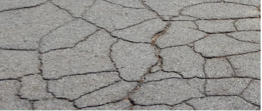
i. Alligator Cracking: Under repeated traffic loads, the series of interconnected cracks on the asphalt pavement surface formed a pattern resembling chicken wire or the skin of an alligator is called the alligator crack or fatigue cracking as shown in Figure 2.1. The alligator cracks are generally occurred under the repeated wheel path.
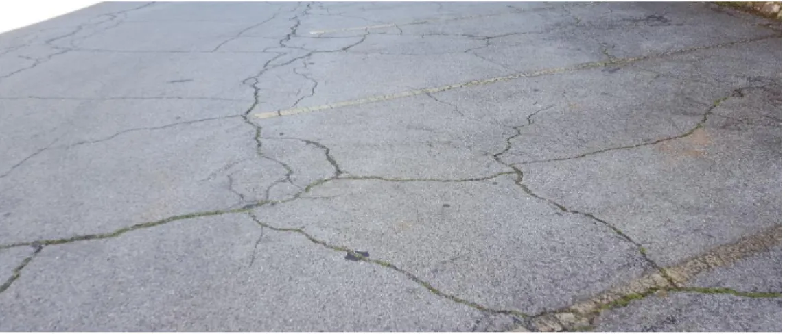
ii. Block Cracking: Block crack looks like the alligator crack, but the block crack is not load associated rather than it caused by the shrinkage of asphalt concrete due to stress/strain temperature cycling. The unit size of the block crack is larger than alligator crack unit and the range of the size is approximately 0.3m to 3m as shown in Figure 2.2. Also, the potential region of the alligator crack is the
repeated wheel load whereas the block area does not occur the wheel load region.
Figure 2.2 Block cracking
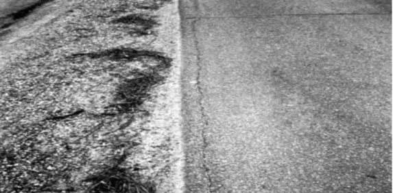
iii. Edge Cracking: Edge cracks are parallel to the outer edge of the pavement and size of the cracks are 0.3 to 0.5m as shown in Figure 2.3 (ASTM, 2011). The edge cracks are occurred due to the weak lateral support, settlement and shrinkage of the subgrade materials Lack of lateral support.
Figure 2.3 Edge crack (ASTM, 2011)
iv. Potholes: Potholes are bowl-shaped depressions generally have size less 30 inches in diameter, sharp edges and vertical sides as shown in Figure 2.4. Pothole creates due to weak pavement surface, excess or deficient of fine materials, as well as poor drainage.
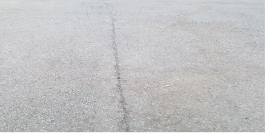
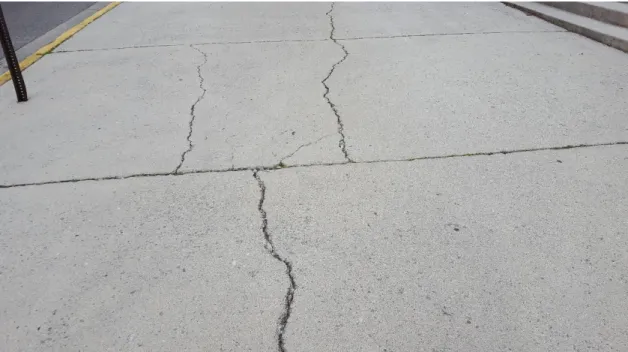
v. Longitudinal Cracking: This crack is parallel to the pavement’s centerline as shown in Figure 2.5. Due to temperature cycling this crack happen in the asphalt concrete (AC) surface. Size and severity of the longitudinal crack are as follows ≤6mm: low, ≤19mm: moderate, >19mm: high (ASTM, 2011).
Figure 2.5 Longitudinal crack
vi. Transverse Cracking: Transverse crack are perpendicular to the pavement
centerline as shown in Figure 2.6. Size and severity of the transverse crack are as follows ≤6mm: low, ≤19mm: moderate, >19mm: high (ASTM, 2011).
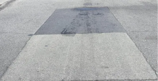
vii. Patching and Utility Cut: The area of a pavement which is replaced by new materials to repair the existing surface as shown in Figure 2.7. This is a defect because it associates with some roughness. Size and severity of the patching and utility cut crack are as follows ≤6mm: low, ≤12mm: moderate, >12mm: high (ASTM, 2011).
Figure 2.7 Patch and utility cut
viii. Rutting: A rut is the longitudinal surface depression along the wheel path which create permanent deformation in the pavement layer as shown in Figure 2.8. The causes of rutting are lateral or consolidated of the pavement material due to traffic load, little compaction in the new asphalt pavement, and plastic fine materials that has low stability to support the traffic. Rutting is obvious after the rain due to water stay on the depressed region. Size and severity of the rutting are as follows ≤6mm to 13 mm: low, >13mm to 25 mm: moderate, >25mm: high (ASTM, 2011).
Figure 2.8 Rutting (ASTM, 2011)
ix. Shoving: The short, abrupt wave in the pavement due to the traffic load is called shoving as shown in Figure 2.9. This distress generally occurs in the cutback or emulsion bituminous pavement.
Figure 2.9 Shoving (ASTM, 2011)
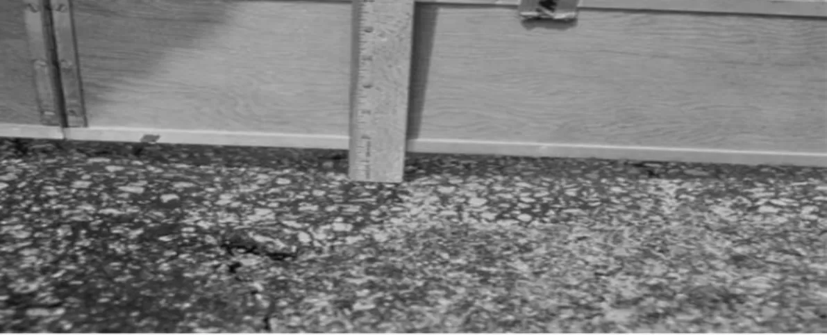
x. Weathering and Raveling: The wearing away of the pavement surface due to the loss of asphalt binder or pavement aggregate is called weather and raveling
distress of the pavement as shown in Figure 2.10. This distress indicates the poor asphalt and binder mixture or hardening of the asphalt due to temperature cycling.
Figure 2.10 Weather and raveling (ASTM, 2011)
xi. Corner Break: Due to the repetition of the load, loss of support and curling stress of slab cause corner break in the rigid pavement as shown in Figure 2.11.
xii. Divided Slab Crack: Due to overloading or loss of support the slab is divided by cracks is called divided slab crack as shown in Figure 2.12.
Figure 2.12 Divided slab crack
2.2 History of Deep Learning
The researcher was trying to find out a computer system that can mimic the biological nervous systems in terms of information processing and communication. In 1986, Rina Dechter introduced Deep Learning to the machine learning community (Dechter, 1986). Igor Aizenberg et. al. first introduced multi-valued neurons and universal binary neurons for the fields artificial neural networks of image processing, control, and robotics as well as pattern recognition (Aizenberg, Aizenberg, & Vandewalle, 2000). In 1973, Ivakhnenko and Lapa published the working algorithm for the supervised, feedforward, deep, and multilayer perceptrons
specially Neocognitron for computer vision (Fukushima & Miyake, 1982). The Neocognitron is a multilayered neural network which has been used for handwritten character recognition and it inspired to developed more advanced convolutional neural networks. LeCun et al. first applied a backpropagation algorithm to recognize handwritten zip code provided by U.S. postal office (LeCun et al., 1989).
Weng et. al. introduced Cresceptron in 1992 which is a hierarchical framework grows automatically using input learning parameters (Weng, Ahuja, & Huang, 1992). At each level of the network, new feature and concepts are detected automatically and the model learning them by creating new neuron and synapses which store new concepts and their corresponding context. The model recognizes the objects and their variations using the learned input knowledge. In 1994, De Carvalho et. al. published 3-layers self-organizing feature extraction neural network module with multi-layer classification neural network module which can train independently (De Carvalho, Fairhurst, & Bisset, 1994).
In 1997 Hochreiter & Schmidhuber introduced long-term-short term memory (LSTM) which eliminate the vanishing gradient problem and can learn very deep task (Hochreiter & Schmidhuber, 1997). In 2015, Google made the LSTM as one of the greatest tools for human speech recognition.
In 2006, Hinton et. al. introduced deep belief nets and they trained the network using unsupervised Boltzmann Machine Learning and then fine tune it using supervised
backpropagation learning (Hinton, Osindero, & Teh, 2006). The deep learning impact on the industry began at the early of 2000 and the large-scale industrial application started around 2010. To make the training process faster, Nvidia launched a graphics processing unit (GPU) in 2009 and Google used the GPU to make a robust deep neural network. The speed of the deep learning
algorithm was increased by 100 times using GPU ("From not working to neural networking," 2018).
2.3 Types of Deep Learning Architectures
The Deep Convolution Networks have dramatically improved the stat-of-the-art of the image processing, video, speech recognition, object detection, as well as visual recognition, whereas the recurrent neural network improved the computation process of sequential data such as speech and text recognition. All the methods of deep learning are the representation-learning methods with composing of non-linear modules transform one level of raw input data to higher level of more abstract data (LeCun, Bengio, & Hinton, 2015). Adam Gibson and Patterson introduced four major architecture of deep networks such as Unsupervised Pretrained Networks (UPNs), Recurrent Neural Networks, Recursive Neural Networks, and Convolutional Neural Networks (CNNs) (Patterson & Gibson, 2017). In this section, more details of the architecture as well as implementations of each of the network will be discussed.
Unsupervised Pretrained Networks
The supervised learning needs lot of data to represent the target objects, for example, the ImageNet dataset used 1M images to train the neural network of 1000 categories. Sometimes, enough data is hard to find and for that the selection of unsupervised neural network is the best option. The goal of the unsupervised learning is to generate a system that can train with little data (Culurciello, 2017). The unsupervised learning has three architectures such as Autoencoders, Deep Belief Networks (DBNs), and Generative Adversarial Networks (GANs) (Adam Gibson & Patterson, 2018).
The autoencoder is an unsupervised neural network which has an input layer, a hidden layer, and a decoding layer. The hidden layer is called encoding layer and this layer should be activated such that it can represent the input parameters to its output. Autoencoder is like PCA (principal component analysis) but it has more flexibility compared to PCA. There are four types of autoencoder such as Denoising autoencoder, Sparse autoencoder, Variational autoencoder (VAE), and Contractive autoencoder (CAE) (Chandrayan, 2017).
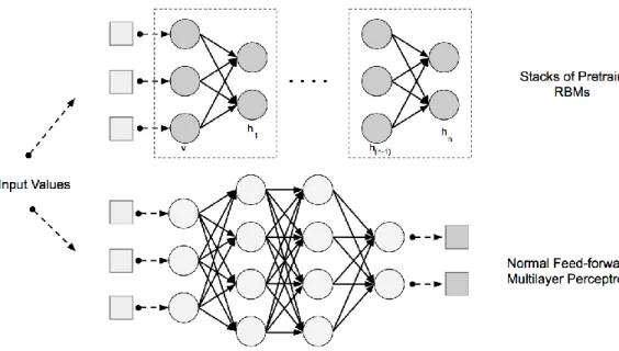
The Deep Belief Network (DBN) used the stacks of Restricted Boltzmann Machines (RBM) layers for pretrain phase and normal feed-forward multiple perceptron for fine-tune phase as shown in Fig. 2.13. From the raw input vectors, the RBM extract the higher-level feature such that the hidden unit reconstruct the input record pretty close to the output records in an
unsupervised training fashion. Each hidden layer of RBM learns more complex high-order feature progressively from the distributed data. These high-order feature layers are used in a backpropagation driven feed-forward neural network as the initial weights. These initialization helps the DBN to fine-tune its parameters (Adam Gibson & Patterson, 2018). The DBN has real-life attractive implementations such as electroencephalography (EEG) (Movahedi, Coyle, & Sejdić, 2018) and drug discovery (Ghasemi, Mehridehnavi, Pérez-Garrido, & Pérez-Sánchez, 2018).
Figure 2.13 DBN model with stacks of pretrain RBM and feed-forward multilayer perceptron (Adam Gibson & Patterson, 2018)
In 2014, Goodfellow et al. introduced Generative Adversarial Nets (GAN) which is a new framework estimating using adversarial process (Goodfellow et al., 2014). This model implements two neural networks simultaneously: one network is called generative model that capture the data distribution and other network is called discriminative model which learns to estimate a sample from the model distribution or the data distribution. In simple word, the generative model is analogous to a team of counterfeiters and it tries to introduce fake currency, whereas the discriminative model tries to detect the falsification and analogues to police or governmental agencies. Two of the model make their best effort until the counterfeits are indistinguishable from the original objects (Goodfellow et al., 2014).
In 2018, GANs were used to paint photorealistic images such as Edmond de Belamy which was sold for $432,500 ("AI Art at Christie’s Sells for $432,500," 2018). Furthermore, GANs have been used for producing the visualization of interior design, bags, shoes, or
computer games scenes. The model also has been used for reconstructing 3D images from 2D image. However, GANs has been used to make false video of Donald Trump and spread in the social media such as Facebook or Twitter (Schwartz, 2018).
Recurrent Neural Networks (RNN)
A recurrent neural network (RNN) is a class of artificial neural network where it
recognizes the sequential characteristics of input dataset and predicts the next probable scenario. The RNN is vast implementations such as robot control (Mayer et al., 2008), time series data prediction (Schmidhuber, Wierstra, & Gomez, 2005), Grammar learning (Schmidhuber, Gers, & Eck, 2002), human action recognition, protein homology detection (Hochreiter, Heusel, & Obermayer, 2007), business process management (Tax, Verenich, La Rosa, & Dumas, 2017), medical care predictions (Choi, Bahadori, Schuetz, Stewart, & Sun, 2016), as well as music composition (Eck & Schmidhuber, 2002).
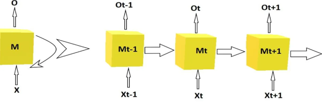
In the traditional neural network, most of the architectures assume that all inputs (and outputs) are independent to each other and they take a fixed-size vector as input and generate fixed-sized vector as output, for example, the Vanilla Neural Network. The recurrent neural network addresses this limitation using the sequential information of an event. The basic RNN architecture is the successive layers of neuron-like nodes where each node relates to the next successive node in a one-way direction. In the architecture, nodes are defined as the input nodes (receiving data from user), output nodes (produced results), and memory nodes (modify and store the information from input to output). The memory unit of the RNN store the information about what has been calculated from the previous input so far and pass it to a successor. An
unfolding typical forward computational diagram is presented in Figure 2.14 where X, M, and O represents the input, memory, and output respectively.
Figure 2.14 Unfolding typical forward computational RNN diagram
Long Short-Term Memory (LSTM) was the first RNN won pattern recognition contest in 2009 (Graves & Schmidhuber, 2009). Google uses LSTM in speech recognition and text-to-speech synthetics (Fan, Wang, Soong, & Xie, 2015). Moreover, combing LSTM with the convolutional neural network dramatically improved the automatic image captioning. It also improved the language modeling (Jozefowicz, Vinyals, Schuster, Shazeer, & Wu, 2016), machine translation (Sutskever, Vinyals, & Le, 2014), as well as multiple language processing (Gillick, Brunk, Vinyals, & Subramanya, 2015).
Recursive Neural Networks
Recursive Neural Network has a tree structure over variable-size input structure in a topological order. The difference between the recurrent neural network and the recursive neural network is that the recurrent neural network used for sequential inputs where the time factor is
the most differential factor whereas the recursive neural network has no time aspect to the input sequence. The input of the recursive neural network must be processed hierarchically in a tree fashion. The recursive neural network is useful for natural language processing.
Goller & Kuchler first introduced the recursive neural network method to solve the tasks consisting of classification of logical terms (Goller & Kuchler, 1996). In the recursive neural network architecture, using the Word2vec function words are converted into the word vector, and this vector is used as the feature and the basis of sequential classification. The word vectors are then grouped into sub phrases and the sub phrases are combined into a sentence. In Figure 2.15, a sentence (represent by S) is sub phrases into the noun phrase (NP) and the verb phrase (VP). By parsing the sentence S, the model creates a tree topology where each parent node has two child leaves (Skymind, 2018).
Convolutional Neural Networks (CNNs)
A Convolution Neural Network (ConvNet) is a deep neural network which is specially implemented for image analysis and it is a class of feed-forward artificial neural network. The architecture of Convolution Neural Network was inspired by biological image processing specially animal visual cortex portion of brain (Matsugu, Mori, Mitari, & Kaneda, 2003). In recent years, ConvNet has been used extensively for face recognition, medical image analysis, scene labelling, image classification, action recognition, human pose estimation, field of speech recognition, text classification for natural language processing, as well as document analysis (Bhandare, Bhide, Gokhale, & Chandavarkar, 2016).
The researcher tried to imitate the human brain image processing techniques into computer vision technology. In 1980, the first Convolution neural network called time delay neural network (TDNN) was introduced (Waibel, Hanazawa, Hinton, Shikano, & Lang, 1990). In 1998, LeCun et al. was the pioneer of the LeNet-5 a seven layer ConvNet for classify hand-written bank checks (LeCun, Bottou, Bengio, & Haffner, 1998). In 2011, Ciresan et al.
implemented GPU for object classification on the NORB, CIFAR10, and MNIST dataset and they got very impressive result with 2.53%, 19.51%, and 0.35% error rate respectively (Ciresan, Meier, Masci, Maria Gambardella, & Schmidhuber, 2011).
The convolution neural network consists of input, hidden, and output layers. The hidden layer composed of serial connection of the feature extraction network and the classification layers. The feature extraction network consists of the pile of convolution, pooling layer, fully connected layer, and normalization layer whereas the classification layer employs the multiclass neural network as shown in Figure 2.16. The convolution layer of the feature extraction network
converts the input image via convolution operation and the pooling layer reduce dimension of the image. The description of convolution, pooling, and fully connected layer are discussed below:
Figure 2.16 Typical ConvNet architecture
The terminology of convolution, pooling, stride and padding, fully connected layer, hyperparameters, Rectified Linear Unit (ReLU), dropout, and data augmentation techniques are discussed below for better understanding of the convolution neural network architectures:
i. Convolution layer: The convolution layer generates feature map using filter called convolution filter. The number of convolution filter and the number of feature map are same. Generally, the convolution filters are two-dimensional matrix, for instances, 5x5 or 3x3 matrices. The matrices values are varied through the training process. The feature map matrices are formed from the multiplication of input image matrices and the convolution filter matrices. The feature maps are then passed through the activation function to the pooling layer as shown in Figure 2.17. The activation function of a node defines as the output of that nodes and it converts the resulting value in the real number domain from 0 to 1 range. Among the Sigmoid, tanh, and Softmax activation function, the most commonly
used activation function is Rectified Linear Unit (ReLU) (B. Xu, Wang, Chen, & Li, 2015).
Figure 2.17 Configuration of convolution operation in the feature extraction network
ii. Pooling Layer: The pooling layer reduces the size of the image through the
process of mean or maximum of the nearest pixel value into a representative value (P. Kim, 2017). Two types of pooling are available such as mean pooling and the max pooling. For the mean pooling the representative value is the mean of all the neighboring pixel value whereat the max pooling is the maximum of the
neighboring pixel value.
iii. Stride and Padding: Stride is the size of the step that a convolution filter moves over the input image matrix. Stride size is 1 in default meaning that the
convolution filter is moving 1 step interval from left to right as shown in Figure 2.18. The more the size of the step is, the less the size of the feature map and the
less overlapping between the cells. Normally the stride size set in a way that the output is an integer instead of a fraction, it can be two or any suitable integer.
Figure 2.18 Yielding of feature map after the implementation of stride and convolution kernel
After the implementation of stride, the dimension of the feature map is reduced, and it lose some feature information compared to the input image. To maintain the same dimensionality, padding is add surrounding the input matrix to prevent the reduction of the spatial dimensionality. The Zero padding adds zero around the border of input matrix and the size of the zero padding can get from equation 1 where K is the filter size and S is the size of the stride (Deshpande, 2018). Zero Padding = (𝐾−𝑆)
2 (1)
The size of the feature map after the zero padding and the stride can be found from equation 2 where O is the feature map height/length, W is the input matrix height/length, K is the filter size, P is the padding, and S is the stride (Deshpande, 2018).
O = (𝑊−𝐾+2𝑃)
𝑆 + 1 (2)
iv. Fully Connected Layer: After the piled of convolution and pooling layer, the fully connected layers make the high reasoning of the classification in the neural network. The layer connects each of the neuron of a layer to the next each neuron of the layer and makes web like a multi-perceptron neural network (MLP). v. Softmax Layer: After the fully connected layer operation, the softmax layer takes
the feature as input and calculates the probabilities as output for each individual class. Then it selects the class of highest probabilities score.
vi. Hyperparameters: The input data can vary by size, complexity and type of image, and more. For that reason, the number of convolution layer, filter size, values of stride and padding varies to get the proper output. The selection of
hyperparameters depends on the right combinations that creates proper scale abstraction of the image (Dertat, 2017).
vii. Rectified Linear Unit (ReLU): The Rectified Linear Unit provides faster training without change in the accuracy compared to traditional activation function and alleviate the vanishing gradient descendent problem. The ReLU activation
function provides faster training compared to sigmoid or tanh activation function. Dahl et al. obtain 4.2% improvement to train a 50 hour English Broadcast News task compared to sigmoid activation function (Dahl, Sainath, & Hinton, 2013). viii. Dropout: Hinton et al. introduced dropout function in 2012 to omit the overfitting
problem (Hinton, Srivastava, Krizhevsky, Sutskever, & Salakhutdinov, 2012). When a large neural network is trained with small training data, the model
half of the neuron is shooting out randomly and it improves the computational time and energy. This powerful technique is called dropout.
ix. Data Augmentation Techniques: The input training data plays a vital role on the model performance. Unfortunately, having a respectable number of data is challenging task. The data augmentation techniques generate data from the existing data using augmentation methods without losing the quality and quantity of the data. Some of the used data augmentation techniques are grayscales, color jitters, horizontal flips, vertical flips, random crops, rotations, and translations. Using this technique, the user can double or triple the input data to feed the network (Pai, 2017).
2.4 Application of Deep Learning Techniques in Civil Engineering
Many researches have been implemented image processing techniques (ITPs) to make the civil infrastructure health monitoring more robust and efficient. Unfortunately, in the real-world situations such as varying lighting condition, noises, shadow condition in images make feature extraction more challenging specially the crack in concrete or rusty steel surfaces. Before the deep learning became popular and robust, different Image Processing Techniques were used to detect and classify pavement cracks. In 2011, Koch and Brilakis used histogram shape-based thresholding, morphological thinning and elliptic regression to detect the pothole in the asphalt pavement (Koch & Brilakis, 2011). However, their model is trained manually, and it detects the pothole based on the geometric shape, texture inside the pothole which is less accurate for the multiple types of cracks. Cord and Chambon proposed AdaBoost based automatic road damage detection method (Cord & Chambon, 2012). AdaBoost (Adaptive Boosting) is a machine
learning algorithm to make an arbitrarily classifier by combining the weak classifier (Freund & Schapire, 1997). Their proposed algorithm could detect the alligator cracks, vertical cracks, horizontal crack and without crack surface in the asphalt pavement. But the algorithm was not robust, and it was not produce the region-based classification and hence it is not useful for practical application. However, German et al. detected region based concrete spalling using a local entropy-based thresholding algorithm (German et al., 2012). Their methodology is applicable for the reinforcement concrete column and it can measure the concrete spalling properties from the image data specially width of the longitudinal or transverse reinforcing steel based on the highly textured regions and ribbed texture along the potentially exposed
reinforcement surface. But their methodology provides overestimation of the spalled regions for the large cracks as the continuation of the spalled region. Liao and Lee proposed a three
techniques such as K-means method in the H component, Double-Center-Double-Radius (DCDR) in Red-Green-Blue (RGB), and DCDR in Hue-Saturation-Intensity (HSI) to detect the rust defects on steel bridge (Liao & Lee, 2016). But the techniques are limited by the images containing coatings on the surface without other objects and the overall accuracy is 86% which is not enough for robust practical application.
Until 2011, deep convolution neural network did not play a vital role in the computer vision, although backpropagation and GPU implementation were been around the decades. In 2012, Cireşan et al. proposed max-pooling convolution neural network on GPU and for the first time the model shows the superhuman performance in the computer vision (Cireşan, Meier, & Schmidhuber, 2012). After the deep learning boom, the researcher from different expertise started extensive use of the convolution neural network to solve corresponding problems such as health risk assessment, drug discovery, natural language processing, image recognition, and so
29
on. Some of the researcher from Civil Engineering expertise used Faster R-CNN deep learning architecture to analyze the railway subgrade defect images taken by the Ground Penetration Radar (GPR). Before the application of deep learning it took long time for the inspector to find out the defects and their types from lot of GPR images. After the application of deep learning algorithm on different types of ground penetrating profile image of subgrade, the Faster R-CNN successfully detect the subgrade settlement defect, water abnormality defect, mud pumping defect, and ballast fouling defect (X. Xu, Lei, & Yang, 2018). Although the method saves time and cost, the limitation of the integration of GPR images with the deep learning algorithm is that the real-time defect detection is not possible, and the integration system is not autonomous. After training the model, the detection process on the test images need GPU based computer system to analyze the recorded GPR images which need also extra cost and expert who knows the deep learning algorithm very well. Soukup and Huber-Mörk trained a Convolution Neural Network to detect the cavities in the rail surfaces from the stereo images (Soukup & Huber-Mörk, 2014). But due to quite small dataset for training, their trained models show approximately 55.6%
overfitting which is worst for real-time application.
Although Cha et al. found 98% accuracy using convolution neural network to detect crack damage detection in concrete surface using realistic situation, their proposed method is applicable for only still images (Cha, Choi, & Büyüköztürk, 2017). Onsite bridge, pavement or any civil infrastructures inspection needs recorded, or real-time video diagnose instead of still images so that it will be more informative for the inspectors. Some researcher applied the
convolution neural network in real-time video analysis to detect the damage in the structures. For Example, Cha et al. trained Faster R-CNN based real-time video based multiple damage
30
delamination, but their algorithm needs simple handy computer chip to apply in practical uses because carrying a laptop webcam or heavy computational equipment is not practical specially in the bridge inspection (Cha, Choi, Suh, Mahmoudkhani, & Büyüköztürk, 2018).
Most of the image processing technique-based research have limitation because of the lack of robust algorithm, enough input image data, low accuracy rate, limited by research objectives, real-time solution is not possible as well as needs costly equipment to implement the research techniques in the practical field. In this research works, seventeen types of pavement crack including eleven types of flexible pavement crack and six types of rigid pavement cracks will study. The objective of this research work is to make a cost-efficient UAV- based
autonomous system using deep convolution neural network and raspberry pi to detect those pavement cracks. After training the convolution neural network, a handy tiny computer
computational chip will be configured so that the inspectors can easily apply the computer vision technique more efficiently as well as in the real-time problem solution.
CHAPTER III METHODOLOGY
This study evaluates different cracks of the pavement using deep learning technology, Unmanned Aerial Vehicle as well as Raspberry Pi. To have an overall idea of this study, a workflow of the proposed UAV/deep learning/Raspberry Pi solution is illustrated in Figure 3.1. Image data used for training and testing of deep neural networks is first collected by using conventional method and UAV carried cameras. Images retrieved by using image search engines may also be used for non-commercial use under the Fair Use Act (Leval, 1990). Images collected will next be labeled by following the ASTM D 6433 standards of pavement distress types.
Thereafter, the labeled image data will be employed to train and evaluate the selected
convolutional neural network by comparing their output losses and accuracy rates. The next step will be to configure a defect detector camera system powered by Raspberry Pi tiny computer with the deep neural network selected in the previous step written to the Pi. After that, the
detector system will be tested by using static images and real-time video. Finally, the UAV/Deep learning/Raspberry Pi detector is ready to mount on a UAV for real-time pavement condition assessment.
Figure 3.1 Workflow of a UAV/deep learning/Raspberry Pi pavement defect detection solution
Prior to implementing the conceptual idea, a pilot study was completed. The training and test images were collected using UAV, Infrared thermography camera, and a handy mobile camera. Bulk Rename Utility ("Bulk Rename Utility," 2019), PixResizer (Groot, 2019), and LabelImg software ("LabelImg," 2018) were used to preprocess the raw images to fit the model. The preprocessed images were split into two groups one for training and the other for testing or validation purpose.
During the training process, a split ratio of 80:20 was applied to a total of 2086
images to divide the training set and the test set images. The input size of images was maintained as 224×224×3 (height×width×channel). In the model used for this study, there are a total of 20 hidden and one input plus one output layers. The pilot study framework is presented in Figure 3.2 to outline the process and methodologies.
Test it in the field and evaluate the efficiency
3.1 Datasets
Image Data Acquisition
Image data needed for training and testing deep neural network were be collected by using a built-in normal image camera on a drone or thermal imaging camera through a gimbal. The DJI Panthom 4 pro with an integrated 20-MegaPixel visual camera and an external 6.8 mm f 1/3 infrared camera used in our study is shown in Figure 3.3. A total of 1500 normal color images and 200 infrared images were collected for annotation. The DJI Go 4 Pro and Flir Vue Pro software were used for controlling drone and thermal camera respectively.
Figure 3.3 Configuration of the drone and the infrared thermal camera for data acquisition
Data Preprocessing
After collecting the images, PIXresizer software ("PIXResizer 2.0.8," 2018) was used to resize image dimension into 838 × 600. Bulk Rename Utility software ("Bulk Rename
Utility," 2018) was used to rename all of the images in numerical order. An open source software labelImg-v1.6.0 ("LabelImg," 2018) was used for labeling purpose. The images were annotated by a total of eighteen (eleven for flexible and six for rigid pavement) different distress types following the ASTM D6433 - 07 standard (ASTM, 2011). The eleven types of flexible pavement distress include transverse crack, edge crack, weather raveling, longitudinal crack, miscellaneous crack, bumps and sags, alligator crack, patch and utility cut, block crack, pothole, rutting, and slippage crack. The rigid pavement images were labeled as divided slab crack, corner break, joint, durability crack, joint spalling, and linear crack. The infrared thermal images were categorized as crack and not crack. During labelling, the unknown cracks were annotated as miscellaneous crack. The sprite image in Figure 3.4 shows some sample data in where first to eighth rows shows the standard images and the ninth to eleventh rows infrared images.
Eighty percent (80%) of all image data were used for training and the rest were for testing and validation. Data augmentation was done using horizontal flipping on the training and validation data set to avoid overfitting as well as to increase the number of images.
Figure 3.4 Sprite image of standard (1st to 8th rows) and thermal image (9th to 11th rows) data
3.2 Evaluation of the Four Real-Time Object Detection Networks
In this work, four recently published object detection meta-architectures including their feature extractor (e.g., Inception, ResNet, MobileNet, NasNet) have been selected and tested, which includes Faster R-CNN (Ren et al., 2015), the You Only Look Once (YOLO) (Redmon et al., 2016), the Single Shot Multibox Detector (SSD) (Liu et al., 2016), and the Region Based Fully Convolution Networks (R-FCN) (Dai, Li, He, & Sun, 2016). Among all these four models, R-FCNN and the YOLO are faster than Faster R-CNN, while Faster R-CNN gives better
accuracy. In fact, the YOLO has the least accuracy of all four models. Meanwhile, the SSD model shows more suitability for android and Raspberry pi applications than the other three models. Some details of the four candidate model architectures are briefly introduced in the following to provide readers with essential background knowledge.
Faster R-CNN
The architecture of Faster R-CNN is divided into two modules/networks: the first one is region proposal network (RPN) that generates region proposals or boxes enclosing objects, which ranks region boxes or anchors and proposes those ones most likely containing objects; the second module of Faster R-CNN includes a classifier for detection and prediction of class label of objects and a regressor used to produce refined bounding box for objects as shown in Figure 3.5. This state-of-the-art real-time object detection neural network reduces running time by sharing full-image convolutional features with the detection network compared to its
predecessors R-CNN (Girshick, Donahue, Darrell, & Malik, 2014) and Fast R-CNN (Girshick, 2015).
Figure 3.5 Faster-RCNN architecture
R-FCN
R-FCN is even faster than the Faster R-CNN without sacrifice of accuracy. This neural network further cuts running time by extracting features of the entire image only once and derives the Region of Interest (RoIs) directly from the feature map instead of computing feature maps for 2000 RoIs. Dai et al. (2016) claimed that R-FCN with the fully convolutional image classifier backbone 101-layer ResNet (He, Zhang, Ren, & Sun, 2016) is 2.5× to 20× faster than Faster R-CNN with the same classifier.
YOLO
The biggest advantage of YOLO (Redmon et al., 2016; Redmon & Farhadi, 2017, 2018) is its very fast speed. This object detection model treats object detection task as a unified
regression problem and predicts bounding boxes and class probabilities directly from full images in only one evaluation with a single neural network, which features fast-real-time speed but the original version YOLO v1 suffers from slightly lower accuracy. Its accuracy has been
and YOLO v3 (Redmon & Farhadi, 2018). It was found that Faster R-CNN is 6 times slower than YOLO (Redmon et al., 2016).
SSD
The single shot detector (SSD) uses only one deep neural network and eliminates the object proposals, which speeds up the computation. Compared to existing methods, a larger number of carefully chosen default bounding boxes are used to improve SSD’s accuracy. In a speed and accuracy comparison study of Faster R-CNN, R-FCN, and SSD, Huang et al. (Huang et al., 2017) show that SSD models with Mobilenet and Inception v2 feature extractor are the fastest and most accurate. Even though SSD performs poorly on smaller object detection, this model is popular for use on Mobile and Raspberry Pi devices due to its fast and lightweight feature extractor.
3.3 Model Hyperparameters
Model hyperparameters such as batch size, learning rate, decay, dropout, and epochs are important parameters need to set. The Intersection of Union (IoU) threshold, image aspect ratio, feature extraction layer, loss function, and matcher are the characteristics parameters that are pre-defined over the training time. Table 3.1 shows the models with their corresponding hyperparameters and characteristics parameters. Equation 3 (Griffiths & Boehm, 2018)
demonstrates the relationship among the training step, learning rate, and decayed learning rate. decayed learning rate=learning rate*decay rate 𝑔𝑙𝑜𝑏𝑎𝑙 𝑠𝑡𝑒𝑝
Table 3.1 Model properties and hyperparameters Model Batch Size Learning Rate (initial) IoU Threshold (1st & 2nd Stage) Feature Extraction layer Image Aspect Ratio Global steps Location Loss Function Matchers Faster R-CNN inception V2 1 0.0002 (0.7 & 0.6) Mixed_4e 600*1 024 60K L2 Argmax Faster R-CNN Nas (Zoph, Vasudevan, Shlens, & Le, 2017) 1 0.0003 (0.7 & 0.6) Mixed_4e 1200* 1200 50K L2 Argmax Faster R-CNN Resnet101 1 0.0003 (0.7 & 0.6) Conv4 600*1 024 50K Smooth L1 Argmax R-FCNN Resnet101 (Dai et al., 2016) 1 0.0003 (0.7 & 0.6) Block3 600*1 024 50K Smooth L1 Argmax
YOLO (Redmon et al., 2016) 64 0.001 -- -- 416* 416 6000 -- Argmax SSD Mobilenet V1 (Huang et al., 2017) 24 0.004 (0.99 & 0.6) Conv_11 and Conv_13 300*3 00 50K Smooth L1 Bipartite SSD Inception V2 (Liu et al., 2016) 24 0.004 (0.99 & 0.6) Mixed_4c and Mixed_5c 300*3 00 50K Smooth L1 Bipartite 3.4 Computational Platform
The network models were programed by using Python 3.6.3 and most of the
experiments were run through the supercomputers at the University of Tennessee at Chattanooga (UTC) Center of Excellence for Applied Computational Science and Engineering (Simcenter). The supercomputer features 33 compute cores, Intel Xeon E5-2680 v4, 2.4GHz chips, 128 GB of RAM, and 1 NVidia 16GB P100 GPU. A high- level neural network computation API Keras ("Keras Documentation," 2018) with backend Google Tensorflow 1.6.0 (Abadi et al., 2016) was used to run the simulations.
CHAPTER IV
RESULTS AND DISCUSSION
This chapter discusses the model selection based on their accuracy and shows the implementation of the selected model in a computer circuit board. The accuracy of the model is determined using the loss parameter. The loss in deep learning is defined as the difference between the predicted and expected outputs, which can be passed on to the optimizer to adjust and update weights in deep neural network. Generally, the lower the loss is, the better a neural network model will be. This work compared the total loss for a total of six object detection network models with respect to epochs and the results are shown in Figure 4.1. In Appendix B, the total loss for each model can be found separately. It is observed that Fast R-CNN with Inception v2 model has the smallest total loss while the SSD with Inception vs performs the worst. The loss of R-FCNN with ResNet 101 reaches minimum after less than 20,000 epochs. It is also noticeable that the total loss of SSD with MobileNet v1 and SSD with Inception v2 is relatively big compared to results using other models.
Figure 4.1 Comparison of total loss of different models
4.1 Real-Time Video Test
The amount of computation time needed is critical for real-time object detection. The lightweight nature of tiny computer motherboards like Raspberry Pi and mobile devices only provide limited computing capability. Therefore, selection of a right detection architecture that achieves satisfying speed and accuracy but with moderate demands of computing is crucial.
The performance was tested for all the seven models shown in Table 1 for one-minute video using GPU equipped laptop using Raspberry Pi 3 B+ camera to compare the mean average precision and real-time speed. These trainable models are publicly available via the Google TensorFlow Object Detection API (Huang et al., 2017). The Inception (Szegedy et al., 2015), NasNet (Zoph et al., 2017), ResNet and MobileNet (Howard et al., 2017) are feature extractors.
It was observed that the SSD with Mobilenet v1 model is most suitable for Raspberry Pi camera, and the rest of the models showed bad memory allocation error due to their heavy inference graph file. Table 4.1 presents the mAP and real-time speed results, which indicate that Faster R-CNN with Inception and ResNet, and SSD with MobileNet models provide best mAP and the combination of SSD with MobileNet yields the fastest real-time speed. The mean average precision (mAP) defines as the average of the maximum precisions at different recall values.
Table 4.1 Comparison of models based on mAP and real-time speed
Models Mean Average Precision
(mAP) Real-time speed (FPS) Faster R-CNN + inception V2 98% 0.5 Faster R-CNN + NasNet 94% 0.01 Faster R-CNN + ResNet101 97% 0.1 R-FCN + ResNet101 87% 0.15 YOLO 26% 5 SSD + MobileNet V1 96% 13.8 SSD + Inception V2 86% 3.6
The authors tested the same pavement at UTC campus real-time distress classification and localization (coordinates of bounding boxes) with different combinations of feature extractor and base architecture: Faster R-CNN with Inception v2 (Figure 4.2), Faster R-CNN with NasNet (Figure 4.3), Faster R-CNN with ResNet101 (Figure 4.4), R-FCN with ResNet101 ( Figure 4.5),
SSD with MobileNet v1 (Figure 4.6), SSD with Inception (Figure 4.7), YOLO (Figure 4.8), and Faster R-CNN with Inception v2 on infrared thermal image (Figure 4.9). The results of
classifications with associated probabilities and localization of the bounding box for the three network combinations are shown in Figures 4.2 through 4.9 where (FP = Flexible Pavement and RP = Rigid Pavement). For example, in Figure 4.2 the associated probabilities of the transverse crack are 99% means that the Faster R-CNN with Inception model can localize the transverse crack with a 99% confident. When the model fails to detect a damage, it assigns a miscellaneous crack name tag on that localized area. In deep learning, localization loss is the difference
between the output or predicted bounding box coordinates and the ground truth of correct box coordinates.
Figure 4.3 Pavement distress classification and localization using Faster R-CNN with NasNet
Figure 4.5 Pavement distress classification and localization using R-FCN with Resnet101
Figure 4.7 Pavement distress classification and localization using SSD with Inception
Figure 4.9 Pavement distress classification using Faster R-CNN on infrared image
It is observed that overall Faster R-CNN with any feature extractors gives the highest confidence level and YOLO generates the worst results. The performance of SSD with MobileNet is comparable to that of Faster R-CNN.
In summary, the overall performance of SSD with MobileNet excels in most of the experiments. Its lightweight nature and fast real-time speed and high precision determine that it is most suitable for running on Raspberry Pi tiny computer powered smart camera detector, which can be deployed for real-time pavement defect detection and localization with speed/accuracy tradeoff.
4.2 Configuration of a Raspberry Pi Camera Module
The proposed smart pavement distress detector camera is built around Raspberry Pi 3 B+ model, equipped with 5MP 1080p HD Video Raspberry Pi camera (Figure 4.10) which supports night vision and can work under any lighting conditions. The total cost of the Raspberry pi
Camera kit took only 317.52$ as described in the table 4.2. The trained SSD with MobileNet neural network for pavement distress detection is fed into Intel® NCSM2450.DK1 Movidius Neural compute stick ("Intel ‑ NCSM2450.DK1 ‑ Movidius Neural Compute Stick," 2018) which is a neural network accelerator that facilitates simple deployment of the deep neural network. An USB-Port-GPS Module with an external antenna can be connected to the
Raspberry Pi motherboard to allow collecting real-time latitude, longitude, and altitude and the GPS coordinates will be received by a receiver on the ground. By adding a USB Wi-Fi network adapter to the Pi motherboard, live pavement defect detection output data can be transferred wirelessly to a receiver on the ground. An overall crack detector system architecture is shown in Figure 4.11.
Table 4.2 Cost of Raspberry Pi crack detector camera kit
SI Product Name Price
($)
Research Use
1 Intel NCSM2450.DK1 Movidius Neural Compute Stick
78.03 It stores the model weight file. The weight file is approximately 10 GB depends on training.
2 6-Inch USB 3.0 Extension Adapter USB 3.0 Port Saver Cable
5.24 Connect Movidious neural stick to Raspberry Pi device.
3 V-Kits Raspberry Pi 3 B+ (B Plus) Complete Starter Kit (16GB & Clear Case Edition)
48.99 Rasberry pi 3+ provides GUI for model implementation.
4 Raspberry Pi Camera 25.99 Takes video input to the model. 5 Ribbon Flat Cable 9.99 Connects Pi Camera to motherboard. 6 7 Inch Capacitive Touch Screen TFT
LCD
75.34 Shows the output.
Total 243.58
Figure 4.10 Raspberry Pi 3 B+ crack detector camera configuration
The preliminary study shows that the Raspberry Pi smart camera can detect and classify pavement distress in real-time with 60% accuracy at 1.20 frame per second (FPS). The accuracy can be improved by using a more powerful model. Although 1.2 FPS is not impressive, it is not necessary to take more than 2 FPS in most flight conditions when used for pavement condition assessment purpose. In Figure 4.12 shows the integration of raspberry pi camera with the drone. There is an external power bank which supplies power to the raspberry pi and the Intel Neural Network Computation stick boost up the image processing speed. Figure 4.13 shows the real-time application of drone pavement inspection using raspberry Pi camera.
Figure 4.13 Drone with Raspberry Pi camera is in action to inspect the pavement defects
4.3 Testing on Real-Time Video
All the models were tested in the real-time situation for one minute using GPU based Laptop building webcam and Raspberry Pi 3 B+ camera. Figure 4.14 compares the image processing speed of different models where SSD Mobilenet V1 has more speed and Figure 4.15 shows the speed of the SSD Mobilenet V1 in Raspberry Pi 3 B+. We found SSD Mobilenet V1 model is suitable for Raspberry Pi camera, and the other models showed bad memory allocation error due to their heavy inference graph file.
Figure 4.14 Comparison of one minute real time speed of different models in GPU based computer
Figure 4.15 One minute real-time speed of SSD Mobilenet V1 in Raspberry Pi 3 B+
4.4 Automatic 3D Drone Mapping Area Calculation
Very few researches have been done to identify the crack in terms of width and length determination using Drone-based application because of inadequate distance measurement tools,
drone noise, and tailored image processing. Kim et al. (2017) proposed a hybrid image processing method incorporating in UAV (H. Kim et al., 2017) to detect the crack dimension. However, as the hybrid image processing method is out of the research scope, we approached the Drone aerial photogrammetry technique. The PIX4D software ("PIX4D-Aerial
Photogammetry," 2018) was used as an autonomous programmed flight path navigator to make the aerial photogrammetric map. The 3D drone mapping was done on UTC Old Library parking space at 50 m drone flight height and 75 to 80% overlapping. After synchronization of 143 images, a 3D photogrammetric map was created using PIX4D cloud. The irregular shapes of crack were annotated, and the crack dimensions were automatically generated based on the annotation as shown in Figure 4.16.