Scene Segmentation and Classification

Scene Segmentation and Classification

J.Sreekanth

A Thesis Submitted to

Indian Institute of Technology Hyderabad In Partial Fulfillment of the Requirements for

The Degree of Master of Technology

Department of Computer Science Engineering

Acknowledgements

Many individuals contributed in many different ways to the completion of this thesis. I am deeply grateful for their support, and thankful for the unique chances they offered me.

Im greatly thankful to my supervisor Dr. C.Krishna Mohan for his valuable guidance, constant encouragement and timely suggestions. I would like to make a special mention of the excellent facility provided to me by IIT Hyderabad.

More than to anyone else, I owe to the love and support of my family. My father J.Venkata Chalapathi, my mother J.Uma and my younger brother J.Prashanth.

Abstract

In this thesis work we propose a novel method for video segmentation and classification, which are important tasks in indexing and retrieval of videos. Video indexing techniques requires the video to be segmented effectively into smaller meaningful units shots. Because of huge volumes of digital data and their dimensionality, indexing the data in shot level is a tough task. Scene classification has become a challenging and important problem in recent years because of its efficiency in video indexing. The main issue in video segmentation is the selection of features that are robust to false illuminations and object motion. Shot boundary detection algorithm is proposed which detects both the abrupt and gradual transitions simultaneously. Each shot is represented using a key-frame(s). The key-frame is a still image of a shot or it is a cumulative histogram representation that best represents the content of a shot. From each shot one or multiple key frame(s) are extracted. This research work presents a new method for segmenting videos into scenes. Scene is defined as a se-quence of shots that are semantically co-related.

Shots from a scene will have similar color content, background information. The similarity between a pair of shots is the color histogram intersection of the key frames of the two shots. His-togram intersection outputs the count of pixels with similar color in the two frames. Shot similarity matrix with 0′sand 1′s is computed, that outputs the similarity between any two shots. Shots are from the same scene if the similarity between the two shots is 1, else they are from different scenes. Spectral clustering algorithm is used to identify scene boundaries. Shots belonging to scene will form a cluster. A new method is proposed to detect scenes, sequence of shots that are similar will have an edge between them and forms a node. Edge represents the similarity value 1 between shots. SVM classifier is used for scene classification. The experimental results on different data-sets shows that the proposed algorithms can effectively segment and classify digital videos.

Key words: Content based video retrieval, video content analysis, video indexing, shot bound-ary detection, key-frames, scene segmentation, and video classification.

Contents

Declaration . . . ii

Approval Sheet . . . iii

Acknowledgements . . . iv

Abstract . . . v

1 Introduction 1 1.1 Motivation . . . 1

1.2 Review of previous work . . . 1

2 Shot Boundary Detection 3 2.1 Feature Vector . . . 3

2.1.1 Static Features of Frames . . . 3

2.2 Types of Shot Transitions . . . 4

2.2.1 Abrupt . . . 4

2.2.2 Graduals . . . 4

2.3 Detection Of Abrupt Transitions . . . 5

2.4 Detection Of Gradual Transitions . . . 5

3 Key Frame Extraction 8 3.1 Alpha Trimmed Average Histograms . . . 8

3.2 Key Frames from a Shot . . . 8

4 Scene Segmentation 10 4.1 Feature Vector . . . 10

4.2 Shot Similarity Matrix . . . 11

4.3 Scene Boundary Detection . . . 11

4.3.1 Spectral Clustering . . . 11 4.3.2 Proposed Algorithm . . . 12 5 Scene Classification 14 5.1 Feature Vector . . . 14 5.2 SVM Training . . . 15 5.3 SVM Prediction . . . 15

6 Experimental Results 16

6.1 Shot Boundary Detection . . . 16 6.2 Scene Segmentation . . . 17 6.3 Scene Classification . . . 18

7 Conclusion and Future work 19

7.1 Conclusion . . . 19

Chapter 1

Introduction

1.1

Motivation

In recent years, due to the wide spread use of digital video technology huge amount of video data is generated. For searching and retrieving it is essential to organize the video data in a efficient manner. The tools used for indexing the video data should be automatic and effective. Segmentation and classification are the basic steps in video indexing. The first step in video segmentation is to segment the videos into elementary units called shots. As the amount of video data available in the web is huge it is difficult for the users to manage the data in shot level. A video contains many shots, thus indexing the data in shot level is quite difficult and ineffective. It is quite necessary for us to shift to next level of indexing i.e., segmentation and classification in scene level. Scene is set of semantically co-related shots. The number of scenes in a video are few, it is easier to manage the data in scene level and the indexing performance increases. Scene segmentation is still a active and challenging research topic. In this work, a new method is proposed for shot boundary detection which is used to identify scene boundaries in the video data and classifying the data using the scene boundaries.

1.2

Review of previous work

Several approaches have been proposed for video indexing. The author in [1], a new method is proposed for video shot boundary detection using early and late fusion, which detects abrupt and gradual transitions simultaneously. A compressed color coherence vector is used as feature vector. The authors in [2] a similarity graph is constructed, in which a shot is represented by a node in the graph and the edges between shots represents the similarity between nodes. The similarity between the shots is calculated using the color and motion information. Normalized cuts [3] method is used to partition the graph, each partition represents a scene. The authors in [4], clustering techniques are applied to cluster shots. A scene transition graph is constructed on the clustered shots, the graph is partitioned into connected sub graphs, each connected sub graph represents a scene. The authors in [5], the background information of each frame is used to segment video into scenes. The idea in this paper is that shots from a scene will have common back grounds. A mosaic technique is used to extract the background information from the images.

similarity matrix is computed between shots using only visual similarity. Similarity matrix is matrix that returns the similarity between any two shots in the video. Spectral clustering algorithm is applied using the similarity matrix to cluster shots into scenes. Sequence alignment algorithm is used to detect scene boundaries accurately. The authors in [7], shots are detected in the video, both the visual and motion features are used to calculate similarity between shots. Shot clustering algo-rithms are used to group shots into scenes. To avoid false positives, an over lapped links methods is proposed which detect scene boundaries accurately. The authors in [8], a scene likeness matrix is calculated that outputs the similarity between shots. A graph is constructed using the scene likeness matrix that similar shots will have an edge between them and graph partitioning method is applied to partition the graph to scenes. The authors in [9][10] similar shots are initially formed into groups, then groups are clustered to scenes. The authors in [11] shot boundary detection technique is used to detect shots. Shots are then clustered using modified k-means clustering.

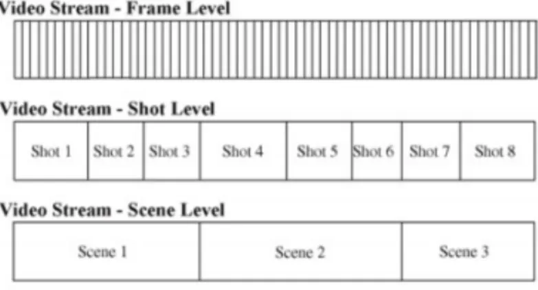
The Figure 1.1 in [12] explains the different levels of decomposition in a video stream.

Figure 1.1: Decomposition levels in video stream.

Frame: Frame is a basic unit of video.

Shot: Shot is sequence of frames that are continuously captured by a single camera. It is an unbroken sequence of frames recorded in a camera.

Scene: Scene is a series of semantically correlated shots. There is no straight forward definition of a scene. Scene usually refers to a group of shots taken in the same physical location.

Chapter 2

Shot Boundary Detection

The important step in video indexing is the detection of shot boundaries in the input video. Frames are extracted from the input video and saved on the disk. Each frame is represented using a feature vector. For all the frames the feature vectors are generated and are stored in an array. The proposed shot boundary detection algorithm which detects both abrupt and gradual transition is explained.

2.1

Feature Vector

Feature extraction is a critical step in content based video indexing. The effectiveness of features shows the effectiveness of the indexing scheme. Audio features and text in the video can also be used for feature extraction, but visual content gives much valuable information.

2.1.1

Static Features of Frames

• Object features: Size, texture, dominant color, are some of the object features. These features retrieve videos that contain similarity between the objects in the videos. Due to advance in technology, faces are now used as objects in video retrieval.

• Motion features: To distinguish dynamic videos from still images these motion features are used. Motion features represent visual content as well as temporal variation of the video. They show the semantic properties of the video and gives more information than the static features.

• Edge features: The edges of an image are used for feature extraction, ECR (edge change ratio) is an edge extraction technique. The advantage of using edge features is that they are invariant to illumination changes and several types of motion.

• Color features: Color moments, color correlograms, color histograms are some of the color based features. The features depends on the color spaces being used, such as RGB, HSV, and YCbCr. The entire frame can be used or the frame can divided into blocks to represent the color features.

In this technique, each frame is represented using a color histogram. For color images, the joint probabilities of the intensities of the three color channels, namely, red (R), green (G), and blue (B) is captured. A 512-dimension RGB color histogram, obtained by quantizing the 3-D color space into

an 8×8×8 grid. A frame is represented using a 24-dimensional feature vector.

Color histograms are widely used for SBD, because they are insensitive to small changes in camera and computationally efficient. But, they lack spatial information i.e. images with different appearances can have the same histogram. In Figure 2.1, there are two different images but they have similar color histograms.

Figure 2.1: Two images with similar color histograms

2.2

Types of Shot Transitions

2.2.1

Abrupt

Cut: In this case there is an abrupt change in frames in which one frame belongs to appearing shot and the previous frame belongs to the disappearing shot. Figure 2.2 shows the abrupt transition between two shots.

Figure 2.2: Abrupt transition between shots

2.2.2

Graduals

• Dissolve: In this case, the last few frames of the present shot overlaps with the few frames of the next shot. The intensity of the frames of appearing shot increases while the intensity of the frames of the disappearing shot decreases and becomes zero.

• Fade: The frames of the present shot gradually fades out into a blank frame and frames of next shot gradually fades in.

• Wipes: In this case the frames of two shots co-exits in two spatial regions. The region of the disappearing shots slowly reduces till it is completely replaced by the appearing shots.

Figure 2.3 from the paper [13], shows the gradual transition between two shots.

Figure 2.3: Gradual change in-between shots

Threshold

Shot boundaries are detected by comparing pair wise similarities against a threshold. The threshold can be global, dynamic/adaptive or combined. In global threshold algorithms, a fixed threshold is calculated and is used for the entire video. In this methods the disadvantage is the local content vari-ations are not incorporated and thus may miss some transitions. In dynamic threshold techniques, a sliding window is created and the threshold is calculated for that window. The performance for dynamic threshold is high and the challenge is to estimate the number of frames in the window. In our experiments, threshold is calculated dynamically and is used to detect the transitions.

2.3

Detection Of Abrupt Transitions

Each frame should be tested to identify the shot boundaries. As explained in [14], let X =

{x1, x2, . . . , . . . , xN_v} is an array of feature vectors of dimension p representing the Nv frames.

Hypothesizing thenth _{frame index, the dissimilarity d[n] between the feature vectors of (n)}th _and

(n−1)th _{frame is calculated asd[n] =d(n, n−1). Euclidean distance, Cosine dissimilarity,}

Maha-lanobis distance are some of the measures used to calculate dissimilarity between frames. Euclidean distance is used as a dissimilarity measure in this method.

Let, d[n] =deuc(xn, xn−1) denote the Euclidean distance between two adjacent feature vectors

xn and xn−1, and σN[n] be the standard deviation of N frames to the left side of framen, then

dynamic thresholdτ[n] is calculated asτ[n] =α×σN[n] whereαis a constant scaling factor.

d[n]> τ[n] (2.1)

An abrupt transition exists at frame indexn, if (2.1) is true.

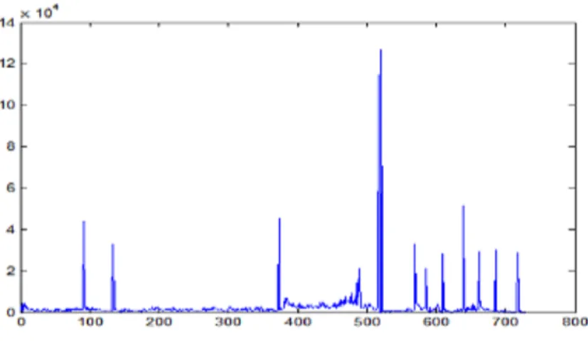
Figure 2.4, shows the sudden change in the peak in the graph when there is an abrupt transition in-between shots.

2.4

Detection Of Gradual Transitions

Both the abrupt and gradual transitions are detected simultaneously. If a transition at nth _frame

is hypothesized as false, the algorithm does not shifts to the next frame, instead the nth _frame

is hypothesized for a gradual transition. The dissimilarity value computed between two adjacent frames is sufficient for the detection of cuts, but fails to identify large number of gradual transitions.

Figure 2.4: Sudden change in dissimilarity measure

In order to identify all the gradual transitions we propose a sliding window technique. During a gradual transition, the adjacent frames does not contribute to the dissimilarity, therefore we have used sliding window technique that considers frames that are separated by a margink.

Suppose we are hypothesizing for a transition at frame index n. Let db[n] be the dissimilarity measure between the feature vectors of framesnand (n₋k) anddf[n] be the dissimilarity measure between the feature vectors of framesnand (n+k). We used euclidean distance as the dissimilarity measure.

Let σL[n₋k+ 1] be the standard deviation of N frames to the left of (n₋k)th _{frame, then}

dynamic thresholdτb[n] is calculated asτb[n] =β×σR[n−k+ 1],β is a constant scaling factor. Let

σR[n+k+ 1] be the standard deviation ofN frames to the right of (n+k)th _{frame, then dynamic}

thresholdτf[n] is calculated asτf[n] =β_×σR[n+k+ 1],β is a constant scaling factor.

Primary condition: The condition for hypothesizing a gradual transition at frame indexnis

db[n]> τb[n] && df[n]> τf[n] (2.2) If (2.2) is true then a gradual transition may exist at frame index n. “&” denotes the standard logicalAN D operator. The condition considers evidence from both sides of a shot boundary, and reduces the miss rate and at the same time decreases false positives.

Entropy: It is a statistical measure of randomness that can be used to characterize the texture of an image. Entropy of a grayscale image is a scalar value. It is defined as

Entropy(I) =∑(−p∗log(p)) (2.3) wherepcontains the histogram counts returned from imhist. LetE be the entropy ofnth _frame.

Secondary Condition:

E_≥6.5 && E_≤7.5 (2.4) A gradual transition at frame indexnis hypothesized as true if both (2.2) and (2.4) are satisfied. “&” denotes the standard logicalAN D operator.

Figure 2.5: Gradual change in the dissimilarity measure in the peak

Figure 2.5 shows the slow change in the dissimilarity measures during a gradual transition curve which requires the use of a window frames.

Algorithm

The entire process of hypothesizing a shot boundary is summarized below.

1. For each frame in the input video sequence, compute thepdimensional feature vector.

2. At frame index n, test the hypothesis as per (2.1).

3. If the hypothesis is true then a cut transition exists, increment n by one and go to step 2. Else, go to step 4.

4. Test the hypothesis as per (2.2). If the hypothesis is true for further validation go to step 5. Else, incrementnby one and go to step 2.

5. Test the hypothesis as per (2.4). If it validates to true then a gradual transition exists at indexn. Else incrementnby one and go to step 2.

Chapter 3

Key Frame Extraction

It is necessary to represent group of frames or shots in a video using efficient and effective descrip-tors. Key frames are still images that best represent the content of the shot. Key frames play an important role in video abstraction process. The efficiency of the abstraction process depends on the key frame extraction method. It is customary to represent the visual and color content of each shot using a frame histograms or key frames. If the shot contains few frames, then one frame can be used to represent the entire shot, but when the frames in a shot are too many then one key frame cannot represent the entire shot, few key frames better represent the content of the shot. In our key frame extraction technique, we have used two key frame extraction methods.

1. Alpha-trimmed average histograms 2. Frames from a shot.

3.1

Alpha Trimmed Average Histograms

As explained in [15], this extraction technique represents the cumulative color information of all the frames in a shot. For all the frames in a shot, accumulate all pixel color values into a single histogram. When normalized the single histogram it produces the average histogram. Each frame in a shot is represented using a 24 dimensional RGB color histogram. The mean of the feature vector for all the frames in a shot is calculated, that single average vector is the key frame that represents the shot. Mean can be replaced by median to produce sample median vector.

AvgHistk(j) = 1 M bk ∑ i=ek Hi(j)j = 1. . . B

where, Hi denotes the histogram ofith frame. M is the number of frames in thekth _{shot. B is}

the total number of bins in the histogram,bk andek are the starting and ending frames of the shot.

3.2

Key Frames from a Shot

The entire shot is represented using a frame(s) from the shot. Only one key-frame is enough if the number of frames in the shot are few. In our method, first, middle and last frames of the shot are

used as key frames. The figures represent key frames from different shots.

Figure 3.1: Key frames from shot 1 and shot 2

Chapter 4

Scene Segmentation

Scene is sequence of semantically co-related shots. Shots in a scene will have similar color infor-mation. In recent years, multimedia applications have been widely used and the amount of digital video data is increasing, there should be efficient tools for retrieving and searching video data. Video abstraction and indexing should be effective and efficient. Shot boundary classification has been used for many years for indexing the video, but as the video data becomes huge it is necessary to shift to next level of indexing i.e., scene classification. Scene boundaries should be identified for scene classification. We already have shots in the input video, from the shot boundaries scenes are identified.

4.1

Feature Vector

In shot boundary detection algorithm, each frame is represented using a 24-dimensional RGB color histogram. This color histograms are simple and computationally efficient. In scene segmentation algorithm, the color histograms for each frame are computed in HSV (HUE-SATURATION-VALUE) with its color co-ordinates uniformly quantized into 12(HUE), 4(SATURATION) and 4(VALUE), a total of 192 quantized color bins is obtained. Each frame is represented as 20 dimensional fea-ture vector. Low level feafea-tures cannot describe the semantic correlation between shots, HSV color histograms gives adequate information about physical setting and connection between shots. HSV color histograms represents the semanticness in the frame better than the RGB histograms which is very crucial for scene detection.

Histogram Intersection

Histogram intersection computes the number of pixels that are common between two images. As already suggested that shots in a scene have similar color content, i.e., they share the same back-ground information. Shots belong to the same scene if the pixels in the backback-ground are same in the shots. The similarity between two shots i.e., the similarity between the key frames should be computed using a metric. Histogram intersection is a metric which outputs the number of pixels common in the two key frames. The pixel count cannot be exactly same, if the two shots have maximum number of pixels common between them then we hypothesize that they belong to the

same scene.

Thekth _{bin value in the intersection histogramIntHistk forn}th_{shot as explained in [15] is given}

by

IntHistn(k) =min{Hi(k)} (4.1) IntHist returns the count of pixels for a single color that appear in all frames.

Threshold

We consider threshold to fill the similarity matrix with o′

s and 1′

s. The experiment is tested for different values of thresholdµ, theµvalue is fixed as 0.75.

4.2

Shot Similarity Matrix

Shot similarity matrix SSM, is a n × n matrix, the values in the matrix represent the similarity between any two shots in the video. The similarity between two shots is calculated using histogram intersection. Each shot is represented using a key frame, every key frame is represented using a HSV color histogram. When the similarity between any two shots exceeds a predefined value then the two shots belong to the same scene.

As suggested in [16], the visual similarity between any pair of shotsi andj is computed as the maximum color similarity among all the possible pair of key frames as

Sim(i, j) = max

p∈Ki,q∈Kj

ColSim(p, q) (4.2)

where Ki andKj are the sets of key-frames of shotsiand j. The color similarity between two framesfi ,fj is given by histogram intersection:

ColSim(i, j) = ∑

h∈bins

min(Hi(h), Hj(h)) (4.3)

whereHi andHj are the HSV normalized color histograms of the framesfi , fj.

Sim(i, j) = 1 if≥0.75 = 0.

4.3

Scene Boundary Detection

4.3.1

Spectral Clustering

Scene detection is difficult task when compared with shot boundary detection, because a scene is a group of shots that are semantically co-related and are continuous in time. Spectral clustering algorithm is used to detect scene boundaries. Clustering is an unsupervised learning classification method. Scene is group of semantically co-related shots. When shots are clustered, shots with simi-larity move to their respective clusters. The steps in spectral clustering algorithm [17] are explained

below.

LetS={s1, s2, . . . , sn}be n shots to be clustered into k groups.

1. Compute the similarity matrixSSM ∈Rn×n _{for all the shots of data setS.}

2. Construct the laplacian matrix L, and D be the diagonal matrix whose (i,i) element is the sum of the i’th row.

3. Compute theK principal Eigen vectors x1, x2, . . . , xk of matrixL to build ann×K matrix

X = [x1, x2, . . . , xk].

4. Re-normalize each row of X to form matrix Y.

5. Cluster the rows ofY into Kgroups using k-means.

6. Assign shotsi to clusterl, if clusterl is assigned a rowi from matrixY.

The main steps in spectral clustering are briefed above. From each shot clustering algorithm estimates the primary color distributions and cluster shots with similar color distributions. The number of scenes and key frames are not equal. The disadvantage of the clustering methods is that the number of clusters has to specified. To resolve this problem, we have used the trial and error method for few videos. Then the number of clusters in a video is less than √n, where n is the number of shots. We proposed a new method to detect scenes.

4.3.2

Proposed Algorithm

To increase the efficiency and to avoid the disadvantage of using clustering method, we have im-plemented a new method for scene detection. The basic idea in this method is that, the sequence of shots with maximum similarity are grouped into a node. Node is a like a subset in a graph or a tree, which has sequence of similar shots from a scene. Hypothesizing a scene boundary at shot l, we have the shot similarity betweenl and the next shot from shot similarity matrix. If the similarity between the shots is zero then the shot itself is the scene, if the similarity is one then the shot l and the next shot belongs to same scene. We continue to check the similarity between shots till the similarity between shots is zero or we reach the last shot. When we encounter the similar-ity between two shots is zero i.e., they belong to two different scenes then we mark a scene boundary.

Algorithm

The proposed scene segmentation algorithm is summarized below,

2. Hypothesizing a scene boundary at shotl, if the similarity between shotsland (l+ 1) is equal to zero go to step 4 . Else, go to step 3.

3. Store the value of variablelto a new variablek. Incrementlby 1 and if the similarity between shotsland (l+1) orkand (l+1) is equal to one, incrementlby 1 and repeat step 3. Else go to step 5.

4. Mark scene boundary from shot l to shotl. Incrementl by 1 and go to step 2.

Chapter 5

Scene Classification

Classification is an important step in video retrieval. The objective of scene classification is to segment the video into scenes, find information and knowledge from the extracted scenes and as-sign videos to predefined categories. Static-based, knowledge-based and machine learning are the approaches used for classification.

• Static-based approach: Videos are classified by statistical modeling video genres. Color statistics, object and camera motion and cuts are analyzed, and these are mapped into film genres.

• Knowledge based approach: This approach gains from domain knowledge and applies heuristic rules to low level features to classify videos.

• Machine learning approach: Samples are labeled and low level features are trained to a classifier or group of classifiers to classify videos.

For scene classification, we used machine learning-based approach. These machine learning techniques uses samples which are labeled with features to train a classifier for a group of videos, the features are extracted for the videos and are classified into their own genre. SVM classifier is used for classification. We considered sports videos for classification, by considering four categories cricket, football, tennis and basketball, including commercials. The videos used for training doesn’t belong to exactly one sports category. The video sequences can be cricket and commercial, football and tennis. Compute the scene boundaries using scene segmentation method described in the previous section, for all the videos to be trained. For all the videos, the frames of the first scene should be saved with a common prefix, the frames of the second scene should be saved with a common prefix and repeat this for all the videos.

5.1

Feature Vector

In this step we extract features from each frame to train the SVM classifier. Histogram of Oriented Gradients (HOG) is used to extract features. HOG is feature descriptor used for object detection. From all the blocks the HOG descriptor returns the vector of the normalized cell histograms. The descriptor is represented by, the count of cells in each block block, the count of pixels in each cell,

the count of channels in each cell histogram. We used 3 cells for each block, number of pixels for each cell are 3, the cell histogram by 9. A 81-dimensional feature vector is generated for each frame. The feature vectors of all the frames are computed and are stored in an array.

Labeling

After computing the feature vector for all the frames, each frame should be labeled accordingly. Labeling helps SVM to distinguish one category to another. All the frames with a common prefix name should be labeled a value, frames from other folder should be labeled other value different from previously assigned value. For all the folders, labels should be assigned. In our experiments we used 2-class svm, we labeled frames from first folder by 1 and frames from second folder as 2.

5.2

SVM Training

In this training phase, the features of the frames are trained to SVM. Two parameters are supplied for svm train function. The first parameter is the array of feature vector of all the frames. The second parameter is the array of the labels of all the frames. SVM assigns the label for each frame and returns a structure which is used as input parameter for svm predict function.

5.3

SVM Prediction

In this prediction phase, video is classified and is assigned to a genre. The video which is to be classified is given as input to the scene boundary detection algorithm and scenes are computed for the video. The frames from the entire video are extracted, for each frame HOG descriptors are computed. An array of HOG descriptors is created. For svm predict function, two parameters have to be supplied. The first parameter is the structure returned from svm training phase and the second parameter is the array of feature vector of the video to be classified. The svm predict function returns an array of labels assigned to each frame. The performance of the classification algorithm is explained in the next section.

Chapter 6

Experimental Results

The performance of each algorithm is explained.

6.1

Shot Boundary Detection

To evaluate the performance of shot boundary detection, the algorithm is experimented on NIST dataset. Total 12 videos are used for testing, consisting of 1461 cuts and 117 gradual transitions. Five other movies are also used for testing. The genre of the movies include action, drama, comedy and thriller.

Recall (R) and precision (P) are the metrics used to calculate the performance of the algorithm, given by recall= Nc Nc+Nm X 100% and precision= Nc Nc+Nf X 100%

whereNmis the actual number of shot boundaries,Nc is the count of shot boundaries which are detected correctly, andNf is the count of false alarms identified. The performance of the algorithm depends on the thresholdα. Ifαvalue is smaller it reduces the precision and increases the recall. A large value ofαincreases the precision and reduces recall value. The measure which is a compromise between precision and recall is given by

F1=

2×R_×P

R+P (6.1)

Ideally,F1should be close to unity. Table 6.1 displays the results for different values ofαandβ.

From the experimental results, for abrupt transitions the optimum value of αis 17, for gradual transitions the optimum value of β is 35. This performance can be improved by using advanced features and by more sophisticated visual similarity measure.

Table 6.1: Performance of shot boundary detection algorithm for different thresholds.

Transition T hreshold Recall P recision F₁

Cut 17 92.19 92.89 92.54 Gradual 35 68.37 68.37 68.37 Cut 15 93.49 91.55 92.50 Gradual 31 69.08 66.66 67.84 Cut 21 91.16 93.33 92.23 Gradual 41 65.81 70.00 67.84

6.2

Scene Segmentation

To evaluate the performance of scene segmentation algorithm, we tested the algorithm on 6 videos from different genres. The video stream is at 25 frames per second, pixel resolution is 320×240, and the video format is AVI. The ground truth of each video is obtained manually. A total of 67 scenes are in the data set. The ground truth of each scene is done manually. Two shot similarity matrices are computed using alpha trimmed histograms as key frames and first, middle and last frames as key frames. The performance of scene segmentation algorithm when spectral clustering algorithm is applied is listed in Table 6.2.

Table 6.2: Performance of spectral clustering algorithm.

Results Recall Precision F1

Alpha Trimmed 74.62 72.72 73.24 Frame from a shot 78.08 77.63 77.85

The performance by using alpha trimmed histograms is very less. In out proposed scene segmen-tation algorithm frames from a shot are used as key frames. The Table 6.3 displays the results of our proposed method for different values of threshold. The performance is measured in recall (R) and precision (P).

Table 6.3: Performance of scene segmentation algorithm.

Threshold(0.70) Threshold(0.75) Threshold(0.80)

Clip ID R P F1 R P F1 R P F1 V1 100 75 85.71 100 100 100 75 100 85.71 V2 80.0 88.88 84.2 90 90 90 70 87.5 77.77 V3 86.66 81.25 83.86 86.66 92.85 89.64 73.33 84.61 78.56 V4 81.48 78.57 79.99 77.77 84.0 80.76 70.37 86.36 77.54 Overall 87.03 80.92 83.86 88.60 91.71 90.12 72.17 89.61 79.94

6.3

Scene Classification

The performance of scene classification algorithm is tested on sports video data-set with four dif-ferent sports categories cricket, tennis, football and basketball. Commercials are also included in the video sequences. For training 2025 frames are used and 1125 frames are used for testing. The same metrics recall (R) and precision (P) are used for measuring the performance of classification. Table 6.4 explains the details regarding the length of each sequence and ground truth of videos classified. The ground truth values of the data set is done manually.

Table 6.4: Duration of segments labeled manually, duration of the segments detected using SVM after applying scene segmentation algorithm.

Ground Truth SVM

Seq No. Class Duration Class Duration Accuracy

1 B 001 –>524 B 000 –>530 (+ 6) Com 525 –>799 Com 531 –>799 2 T 001 –>492 T 001 –>484 (- 8) F 493 –>1012 F 485 –>1012 3 C 001 –>550 C 001 –>546 (- 4) Com 521 –>750 Com 547 –>750 4 F 001 –>510 F 001 –>522 (+ 12) T 525 –>799 T 523 –>799

The overallF1measure of all the data set is 93.36%.

Class notation C: cricket, B: basketball, T: tennis, F: football, Com: commercial.

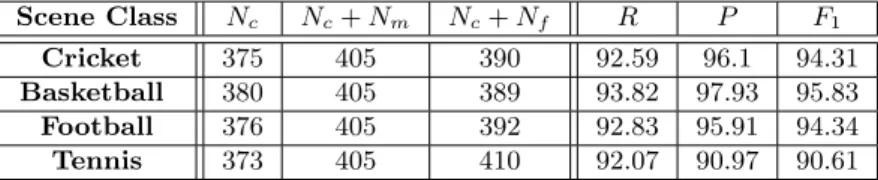
The experimental results in Table 6.5 gives theF1measure of each sports data set and shows the

effectiveness of our scene classification algorithm. For basketball data set the classification results are the best. In tennis data set, the ground color in the videos is both green and brown, the svm has classified some of the frames of tennis data set as cricket, the performance of tennis data was less.

Table 6.5: Performance of Scene classification algorithm.

Scene Class N_c N_c+N_m N_c+N_f R P F₁

Cricket 375 405 390 92.59 96.1 94.31

Basketball 380 405 389 93.82 97.93 95.83

Football 376 405 392 92.83 95.91 94.34

Tennis 373 405 410 92.07 90.97 90.61

Chapter 7

Conclusion and Future work

7.1

Conclusion

In this thesis work a new method for scene segmentation and classification is proposed. Initially shot boundaries are detected. From the shot boundaries, scenes are identified in the videos. Using the scene boundaries the videos are first trained and then classified using SVM. The presented experimental results proves that the proposed method detects scene boundaries and classifies the videos accurately. The performance of the proposed algorithms can be used by using advanced feature extraction techniques.

References

[1] C. Krishna Mohan. “Features For Video Shot Boundary Detection And Classification” .

[2] Z. Rasheed and M. Shah. “Detection and representation of scenes in videos”. Multimedia, IEEE

Transactions on 7, (2005) 1097–1105.

[3] J. Shi and J. Malik. “Normalized cuts and image segmentation”. In Computer Vision and Pattern Recognition, 1997. Proceedings., 1997 IEEE Computer Society Conference on. 1997 731–737.

[4] M. Yeung, B.-L. Yeo, and B. Liu. “Segmentation of Video by Clustering and Graph Analysis”.

Computer Vision and Image Understanding 71.

[5] L.-H. Chen, Y.-C. Lai, and H.-Y. M. Liao. Movie scene segmentation using background infor-mation. Pattern Recognition 41, (2008) 1056 – 1065. Part Special issue: Feature Generation and Machine Learning for Robust Multimodal Biometrics.

[6] V. Chasanis, C. Likas, and N. Galatsanos. “Scene Detection in Videos Using Shot Clustering and Sequence Alignment”. Multimedia, IEEE Transactions on 11, (2009) 89–100.

[7] X. Wang, S. Wang, H. Chen, and M. Gabbouj. “A Shot Clustering Based Algorithm for Scene Segmentation”. In Computational Intelligence and Security Workshops, 2007. CISW 2007. International Conference on. 2007 259–252.

[8] H. Lu and Y.-P. Tan. “An efficient graph theoretic approach to video scene clustering” 3, (2003) 1782–1786 vol.3.

[9] S. Liu, M. Zhu, and Q. Zheng. “Effective video content abstraction by similar shots clustering” 1445–1448.

[10] W.-G. Cheng and D. Xu. “Content-based video retrieval using the shot cluster tree” 5, (2003) 2901–2906 Vol.5.

[11] P. Mohanta and S. Saha. “Semantic Grouping of Shots in a Video Using Modified K-Means Clustering” 125–128.

[12] P. Sidiropoulos, V. Mezaris, I. Kompatsiaris, H. Meinedo, M. Bugalho, and I. Trancoso. “Tem-poral Video Segmentation to Scenes Using High-Level Audiovisual Features”. Circuits and

[13] C. Cotsaces, N. Nikolaidis, and I. Pitas. “Video shot detection and condensed representation. a review”. Signal Processing Magazine, IEEE 23, (2006) 28–37.

[14] C. Krishna Mohan, N. Dhananjaya, and B. Yegnanarayana. “Video Shot Segmentation Using Late Fusion Technique” 267–270.

[15] A. Ferman, A. Tekalp, and R. Mehrotra. “Robust color histogram descriptors for video segment retrieval and identification”. Image Processing, IEEE Transactions on11, (2002) 497–508.

[16] V. Chasanis, A. Likas, and N. Galatsanos. “Scene Detection in Videos Using Shot Clustering and Symbolic Sequence Segmentation”. In Multimedia Signal Processing, 2007. MMSP 2007. IEEE 9th Workshop on. 2007 187–190.

[17] V. Chasanis, A. Likas, and N. Galatsanos. “Efficient Video Shot Summarization Using an Enhanced Spectral Clustering Approach”. In Proceedings of the 18th International Conference on Artificial Neural Networks, Part I, ICANN ’08. Springer-Verlag, Berlin, Heidelberg, 2008 847–856.