Linearizing Convolutional Neural Network improves P300 detection

UC San Diego

UC San Diego Electronic Theses and Dissertations

Linearizing Convolutional Neural Network improves P300 detection Permalink https://escholarship.org/uc/item/0z42g434 Author Ravindran, Sriram Publication Date 2018 Peer reviewed|Thesis/dissertation

UNIVERSITY OF CALIFORNIA, SAN DIEGO

Linearizing Convolutional Neural Networks improves P300 detection

A Thesis submitted in partial satisfaction of the requirements for the degree

Master of Science in Computer Science by Sriram Ravindran Committee in charge:

Professor Virginia de Sa, Chair Professor Garrison W. Cottrell Professor Lawrence Saul

Copyright Sriram Ravindran, 2018

Signature Page

The Thesis of Sriram Ravindran is approved, and it is acceptable in quality and form for publication on microfilm and electronically:

Chair

University of California, San Diego

DEDICATION

I dedicate this thesis to my family, friends and my advisor. My family, for making me the person I am.

My friends, for their company and support. My advisor, for having confidence in me.

TABLE OF CONTENTS

Signature Page ... iii

Dedication ... iv

Table of Contents ... v

List of Figures ... vii

List of Tables ... viii

Acknowledgements ... ix

Abstract of the Thesis ... ix

Chapter 1 - Introduction ... 1

1.1 P300 ... 3

1.2 P300 Spellers ... 4

1.3 EEG Signal Analysis using Machine Learning ... 6

1.3.1 Traditional Approaches ... 6

1.3.2 Deep Learning in the last decade ... 6

1.4 Objective ... 7

1.5 Organization of the thesis ... 8

Chapter 2 - Background and related work ... 9

2.1 Literature Review ... 9

2.2 Basics of Neural Networks and Deep Learning ... 12

2.2.1 Neural Networks ... 12

2.2.2 Convolutional Neural Networks ... 15

2.2.3 2D Convolution ... 17

2.2.4 3D Convolution ... 18

2.2.5 Batch Normalization ... 19

2.3 Interpretability ... 20

2.3.1 Converting backward models to forward models ... 21

Chapter 3 - Methods:Pre-processing and classification ... 22

3.1 P300 Dataset ... 22 3.2 Objective ... 24 3.3 Data pre-processing ... 24 3.4 Popular Architectures ... 27 3.4.1 EEGNet ... 27 3.4.2 CecottiNet ... 28 3.5 Architectural Tests ... 29

3.5.1 Square kernels ... 29

3.5.2 Linear activation function ... 30

3.5.3 Spatio-temporal kernel ... 30

3.5.4 Large temporal convolutions ... 31

3.5.5 Average pooling ... 31

3.5.6 Network size ... 31

3.5.7 Using 3D data ... 32

3.6 Knowledge distillation ... 32

Chapter 4 – Experimentation, results and discussion ... 34

4.1 Experimental Setup ... 34

4.2 Results ... 36

4.3 Visualization ... 38

Chapter 5 – Conclusion and future work ... 41

LIST OF FIGURES

Figure 1.1 Working of a brain-computer interface taken from [1] ………. 2

Figure 1.2 BCI Speller proposed by and taken from [8]………. 4

Figure 2.1 A single hidden layer feedforward neural network……… 13

Figure 2.2 Shared parameters and local connectivity……….………. 15

Figure 2.3 Pooling operations……….. 16

Figure 2.4 Working of a 2D convolution layer………... 17

Figure 3.1 Location of the electrodes on the scalp……….. 23

Figure 3.2 Results of the 3D to 2D projection process……… 26

Figure 3.3 Exponential Linear Unit………. 28

Figure 4.1 Activation pattern learned by EEGNet+ for Subject A……….. 38

Figure 4.2 Activation pattern learned by EEGNet+ for Subject B……….. 38

Figure 4.3 Activation pattern learned by Shrinkage LDA for Subject A with 10 buckets………... 39

Figure 4.4 Activation pattern learned by Shrinkage LDA for Subject B with 10 buckets………... 39

LIST OF TABLES

Table 3.1 Architecture of EEGNet……….. 27 Table 3.2 Architecture of CecottiNet……….. 28 Table 4.1 Performance measure for various classifiers for Subject A (details in

section 4.2) ………. 36 Table 4.2 Performance measure for various classifiers for Subject B (details in

section 4.2) ………. 37 Table 4.3 Performance measures for CecottiNet……… 37

ACKNOWLEDGEMENTS

I want to thank the committee members for generously donating their time and knowledge. I thank my advisor and committee chair Prof. Virginia de Sa for the opportunity to work in her lab and her guidance throughout this project. I thank my lab members Ramesh Krishna, Mahta Mousavi and Shuai Tang for their guidance, especially Ramesh for providing starter code. I thank Prof. Garrison Cottrell and Prof. Lawrence Saul for agreeing to be part of my M.S. thesis committee.

Chapter 3, in part, was submitted to BCI Meeting 2018, Ravindran, Sriram; de Sa, Virginia R. The thesis author was the primary investigator of this material.

Chapter 4, in part, was submitted to BCI Meeting 2018, Ravindran, Sriram; de Sa, Virginia R. The thesis author was the primary investigator of this material.

ABSTRACT OF THE THESIS

Linearizing Convolutional Neural Network improves P300 detection

by

Sriram Ravindran

Master of Science in Computer Science

University of California, San Diego, 2018

Virginia de Sa, Chair

P300 is an event-related potential evoked as a response to external stimuli. The P300-speller is a widely used BCI that has proven to be a reliable method in enabling people who cannot communicate via normal methods. Improving single-trial P300 classification helps

increase communication bandwidth as it reduces the averaging process necessary to reduce noise. Deep learning approaches in this area have become more popular recently [2][3]. Certain architectural choices result in a better classifier. In this paper, we performed a study of EEGNet [2] as it performed well in our experiments. We report some improvements to the model. We also confirm that these suggestions improve other CNN based models by showing improved results with CNN-1 proposed in [4] on BCI Competition III Dataset II. We perform knowledge distillation of the resultant linear model into a logistic regression model and show that the model learns information similar but superior to LDA. We show that the logistic regression model obtained this way outperforms more complex models and is easy to interpret.

Chapter 1

Introduction

Brain Computer Interfaces (BCI), also called Direct Neural Interface or Brain-machine interface is a technology that allows a human to communicate with an artificial device. Typically, brain signals are captured using electrodes, processed, and using complex algorithms, used to control external devices. Thus, it is used most commonly to augment or repair cognitive functions, particularly in persons with locked-in syndrome, who have lost the ability to control their muscles and are effectively paralyzed. While BCI can be invasive – using electrodes implanted inside the skill – this work relates to using signals collected non-invasively.

To record the electrical activity of the brain, we use Electroencephalography(EEG). It works by placing electrodes on the scalp, which measure the voltage fluctuations resulting from electrical activity of the neurons that lie below. There are other methods to capture brain function, including fMRI (functional Magnetic Resonance Imaging), positron emission tomography, magnetoencephalography (MEG). Each of these techniques offer some benefit

at some cost. EEG is a good choice for the study of brain function because it has multiple advantages; it is cost effective [5], easy to transport, has high temporal resolution [6], does not trigger claustrophobia [7] unlike fMRI and PET scans, and most importantly, is non-invasive. However, it also has certain glaring disadvantages; poor spatial resolution [8], poor signal-to-noise ratio and a non-stationary time series. It also requires precise placement of electrodes and any disturbance in the placement of electrodes can affect analysis but doesn’t provide any information on which structure of the brain the signal is coming from. It is also susceptible to various artifacts that are not related to the event that the brain is responding to, for example, flickering of the eyelids, and facial muscular activity. Despite its poor spatial resolution, it still provides enough information for it to be a natural choice for many day-to-day applications.

Figure 1.1 Working of a brain-computer interface taken from [1]

The signals are collected from the human scalp using electrodes placed according to a fixed pattern. This signal is then amplified and digitized using an analog to digital converter. The next step in classical machine learning is to extract features manually and

feed them into a classifier that learns to separate the data into different classes. Often, this feature extraction step is trivial, and the data is directly fed into the classifier. Once the classification is done, the output is given to the user as feedback.

Brain computer interfaces have huge applications. Some examples include communication for people locked-in syndrome, ability to control prosthetic devices, rehabilitation after neurological diseases, entertainment and gaming, lie detection, sleep-monitoring, driver alertness checking and many more. In this work, we focus on one kind of ERP (Event-related potential) found in EEG, called the P300 and the primary application discussed is a speller device.

1.1

P300

There are several categories of EEG based BCIs, namely P300 [9] [13], steady state visual evoked potential (SSVEP) [10], event related desynchronization (ERD) [11] and slow cortical potential based BCIs [12]. This work relates to P300 based BCI. The P300 is an ERP that is widely used in BCI. These are signals that are evoked as a response to an external stimulus. When recorded using an EEG device, it presents itself as positive deflection. It is commonly elicited during an “oddball” paradigm, which is when a subject detects a target stimulus in an otherwise standard setting. It is important to note that the P300 is elicited only when the subject is actively participating in the task of detecting the target stimulus. Figure 1.2 shows what a standard P300 signal looks like. The more improbable the target stimulus, the larger the amplitude of the P300 is. Typically, among young adults, the P300 signal peak presents itself at about 300ms after the event. However, in patients with decreased cognitive

ability, this could vary and the P300 could be smaller. The exact origin of the P300 in the brain is unknown, but the hippocampus and the associated areas in the neocortex are believed to contribute to the P300 signal [14].

1.2

P300 Spellers

Figure 1.2 BCI Speller proposed by and taken from [9]

While the P300 has many applications, the P300 speller is a popular and effective BCI system that allows people with locked in syndrome to type with their thoughts. The idea is to elicit large differences in target and non-target ERPs. This is done by displaying a visual

paradigm on a computer screen. The most common P300 speller was the earliest one, proposed by [9] shown in Figure 1.2

The speller consists of a 6 x 6 matrix of symbols that comprise of alphabets A-Z, and numbers 0-9. The user of the system is asked to think of the character he/she wants to spell and look out for the corresponding row and column flash. The rows and columns are flashed in a random order. Whenever the the row/column contains the character that the user wants to communicate, a P300 is elicited. This process is usually performed multiple times and the results averaged. The row and column with the highest P300 peaks are selected and this determines the letter the user wants to communicate – the one in their intersection.

The hallmark of a P300 based BCI Speller is that it doesn’t require extensive user training, as the P300 is elicited out of a natural brain response to the experiment. However, an averaging process is required to tackle the problem of low signal-to-noise ratio. The same experiment is performed multiple times and the signals averaged. This reduces the rate at which the user is able to communicate. There is also the problem of an underlying changing distribution. The person using the system may have varying levels of motivation, attention, fatigue and interest [15]. The P300 is not common either, although its form is roughly similar it is somewhat unique to each person. Therefore, any speller system based on P300 must be tuned to each user. Even if efforts are taken to correct these issues, P300 speller present the problem of low real-time accuracy. This has been addressed in [16, 17, 18, 19] by dividing computer screen into multiple regions. To combat this, it is useful to classify raw P300 i.e., classify the raw signals (with low signal-to-noise ratio) without averaging. This is called single-trial EEG classification.

1.3

EEG Signal Analysis using Machine Learning

1.3.1

Traditional Approaches

The most common method for single-trial EEG classification is Linear Discriminant Analysis. Since the number of features for each trial is N (number of time points) x C (number of channels), it suffers from the curse of dimensionality. We do not possess enough data to counter this either as data collection is a time-consuming process. Therefore, each trial is time-windowed with 5 or 10 buckets. For P300 based systems, since the peak is expected in the midline parietal regions, only a few channels in and around this region (particularly Cz, Cpz) are chosen. This way the dimensionality is reduced drastically. Fisher’s LDA (Linear Discriminant Analysis) has been used in motor imagery based BCI [20], P300 spellers [21] and multiclass [22] BCI. Regularized versions of LDA used in [23] provide better results than normal LDA, but are not commonly used in BCI applications. Another common approach is SVM, which is a linear classifier when a linear kernel is used. As stated in studies [24, 25, 26], linear approaches based on SVM and LDA outperform simple non-linear approaches like MLP and even kernelized SVM. Our previous work [27] improved upon linear approaches by proposing a deep recurrent non-linear network that outperforms LDA approaches.

1.3.2

Deep Learning in the last decade

In the last decade, deep learning has become very popular. Deep learning refers to the use of deep neural networks to automatically learn features as opposed to engineering them by hand. They have transformed the field of Computer Vision and NLP and are being

applied in more and more areas. This could be useful in the context of EEG analysis because EEG is not easily interpretable; in contrast, images or audio can be deciphered by seeing or listening respectively. Therefore, it might be meaningful to let the algorithm decide the features it needs to extract for best classification performance. So far, the spatial and temporal structure of EEG has been largely ignored. Convolutional Neural Networks (CNNs) [28, 29] can help us capture the spatial structure of EEG while LSTMs [30] are useful in capturing the temporal structure.

1.4

Objective

The purpose of this work is to build simpler and more effective classifiers than our previous work [27]. In general, almost all approaches in EEG analysis simply convert the spatio-temporal signal to a one-dimensional vector. This removes any spatial or temporal structure the network might have. Imposing constraints on the network to exploit this structure might enable the networks to build better classification boundaries.

The deep networks we designed in the past have the ability to extract spatial and temporal structure of the data. In this work other popular deep learning approaches like [2] and [4] are analyzed for architectural choices that enable them to work well. New measures are proposed which further improve these networks. We show that some of these measures, which improve one network also improve other networks, implying that the measures proposed are not unique to the networks being analyzed.

Aside from this analysis, another network that uses spatial structure of EEG has been constructed. The effectiveness of each classifier is compared over various measures.

Furthermore, based on the discovery that linear CNNs are most effective in this task, an equivalent logistic regression model is generated. Using visualization methods proposed by Haufe et al. [31], backward models like logistic regression and LDA are converted to forward methods and the activation patterns that these models are looking for are compared. A description of backward and forward model is presented in section 2.3.1.

1.5

Organization of the thesis

The report is organized as follows: Chapter 2 contains relevant background and literature review on EEG signal classification with traditional and deep learning methods. It also describes the basics of neural networks and deep learning. Chapter 3 provides some details on the dataset and the improvements to the model along with backward to forward model conversion. Chapter 4 provides the results of the proposed model and compares it with Shrinkage-LDA and also contains the visualizations of the patterns learned by these models. Chapter 5 concludes the thesis and mentions possible future work.

Chapter 2

Background and related work

2.1

Literature Review

P300 classification has become more popular since mid 2000s. A comparative work is by Rusenski et al. [32] who tested five methods – Pearson’s correlation method (PCM), Fisher’s linear discriminant (FLD), stepwise linear discriminant analysis (SWLDA), linear support vector machine (LSVM) and Gaussian support vector machine (GSVM) – for the purpose of classification of P300 speller data. The reason for choosing these models were that PCM and FLD were simple linear methods, whereas SVMs and LDA methods were chosen as complex linear methods. GSVM was chosen to evaluate the benefit of kernel methods. They found that FLD and SWLDA are the best performers, this was attributed to the fact that FLD accounts for the covariance between features and that SWLDA solves the problem of large feature spaces by selectively limiting the size of the input feature space. Although SVMs in general perform well due to the desirable theoretical property and the advantage of maximizing the margin between classes, they did not perform as well as

expected. GSVMs performed inferior to LSVM, which is attributed to overfitting and are not desirable due to increased training time.

Manyakov et al. [25] performed a similar experiment but on disabled subjects. They tested Bayesian linear discriminant analysis (BLDA), SVM, Fisher’s LDA, SWLDA, Linear SVM, multi-layer perceptron MLP, and GSVM. According to their results, BLDA yielded the best results, with SVM as the second best. In a study by Marchese et al. [26], Fisher LDA outperformed LSVM, GSVM and MLP. This leads us to believe that LDA approaches are particularly well suited for P300 classification tasks. Although [27] describes a non-linear network that works better than LDA, linear algorithms seem preferable.

The field of deep neural networks has exploded with each new work besting the previous. Following the success of deep learning models in other areas, it has been applied to EEG classification as well. Cecotti et al. [4] used convolutional neural networks for P300 classification. The dataset used was the BCI Competition III Dataset II [33] where they constructed a classifier first and used it to determine the sequence of alphabets the user was thinking of during the experiment. This work is explained in greater detail in Section 3.4.2. In short, they use 2 convolutional layers, followed by a fully connected layer. The network uses temporal structure of EEG but does not use spatial structure of EEG, therefore, any permutation of the electrodes yields the same performance.

In another convolutional network based model by Mirowski et al. [34], the network was used to predict epileptic seizures. This is a popular application of machine learning to EEG data. The performance of the networks was compared with linear models like SVM and logistic regression. The model used by them is invariant to temporal shifts in the data.

Although this could be meaningful for certain applications, it is not the case with P300. The P300 signal is a positive inflection expected around 300ms after the stimulus. Bashivan et al. [35] used a convolutional network with recurrent units to learn both spatial and temporal structures in EEG data for mental load classification. In addition, they also preserved spectral structure of EEG. To do this, they used a technique called as Azimuthal Equidistant Projection (AEP) which projects the 3D EEG data onto a 2D surface, similar to how a globe is projected to create a map. Thereafter, they interpolated between the electrodes to obtain a 32x32 grid. They projected the power values in different frequency bands alpha, beta and theta and used them as different channels in the input similar to the idea of RGB channels in images. These inputs were fed to feedforward CNN models and also CNNs with LSTM units. They found that while the CNN works very well, the best performance was achieved when the features extracted by the CNN were fed to the LSTM units. We have tried the same technique – AEP – in this work. However, we project the electrode potentials instead of power values.

Maddula et al. [27], applied a similar method for P300 classification. We performed AEP of the data to produce a time series of images, and treated the task similar to video classification. We averaged each trial into 5 or 10 buckets for subsampling, and fed each bucket to a CNN. The outputs from these CNNs were fed into an LSTM to learn the temporal patterns. Thereafter a 3D CNN was added on top of the 2D CNN to learn spatio-temporal features. We found that the 3D CNN performed the best amongst all the models, including shrinkage LDA. We also used transfer learning to first train a classifier that is not specific to any subject and the fine-tuned the weights to work well for one subject in particular.

EEGNet [2] is a very simple convolutional network, that emphasizes having a low number of parameters and thus avoids the use of fully connected layers. They demonstrated good performance on multiple datasets involving different types of ERPs. EEGNet was proposed as a general-purpose architecture for EEG classification tasks, however we found that it can be improved significantly. The architecture of EEGNet is explained in greater detail in section 3.4.1.

Schirrmeister et al. [36], investigated deep ConvNets with different architectures for decoding motor imagery data. They proposed both shallow and deep convolutional architectures, and found that both architectures are either close to, or slightly better than FBCSP (Filter bank common spatial patterns), the de facto standard for motor imagery tasks. They also introduced a new method of feeding data to the network, called cropped training to combat overfitting issues. They found that ELUs perform significantly better than ReLUs for EEG tasks but this difference is not found in computer vision tasks [48]. Furthermore, they proposed a correlative and causally interpretable visualization method to visualize the frequencies and spatial distribution of band power features. In our work, we propose a much simpler method by taking advantage of the linear nature of our final model.

2.2

Basics of Neural Networks and Deep Learning

2.2.1

Neural Networks

Artificial neural networks (denoted henceforth as neural networks) are a class of machine learning algorithms inspired by biological neural networks. The fundamental component of a neural network is an artificial neuron which is a simplified version of a

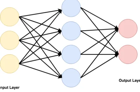
biological neuron. A directed, weighted graph of such neurons is constructed where each neuron accepts inputs, performs a linear weighting – defined by the graph weights – of the inputs and might apply a non-linearity. Figure 2.1 shows the structure of a single hidden layer feedforward network. The network takes in 3 dimensional vectors as inputs, and contains one hidden layer with 4 hidden neurons and two output neurons.

Denoting the input vector as X = [x1, x2, … xn], and all parameters associated with

the input layer with subscript i, hidden layer with subscript j and output layer with subscript

k, and G being the activation function, the equations related to the forward pass are presented below.

Figure 2.1 A single hidden layer feedforward neural network

𝑝_𝑗 = 𝑤_𝑖𝑗.𝑥_𝑖 𝑛

𝑖 = 0

+𝑏_𝑗

where, pj is the linear sum of input values weighted by 𝑊:𝑗(the j'th row of Wi) 𝑞_𝑘 = 𝑤_𝑗𝑘 𝑛ℎ 𝑗 = 0 .𝑧_𝑗+𝑏_𝑘 𝑧_𝑘 = 𝑮(𝑞_𝑘)

Note that each neuron has its own bias, therefore bj is not a unique bias value for the

hidden layer, but the bias of the hidden neuron currently being looked at. Traditionally, to convert the activations of the final layer neurons into class probabilities, a softmax function is used as shown below,

𝑦_𝑘 = 𝑒

𝑞𝑘 𝑒𝑞_𝑙 𝑙

Various error metrics have been used for different purposes, but the most common error metric used for measuring classification performance is Cross-Entropy Loss. The final loss of the binary classification network as presented in Figure 2.1 is given below.

𝐽 𝑥,𝑦,𝑊_𝑖,𝑊_𝑗 = − 𝑦_𝑘ln 𝑦_𝑘 𝑘

Once the forward pass of the network has been performed, a loss function J is computed. For each weight, the following updates are performed.

𝑤_𝑖𝑗 ← 𝑤_𝑖𝑗 − 𝛼 𝑦_𝑘 1− 𝑦_𝑘 𝑤_𝑗𝑘𝐺′ _𝑝 𝑗 𝑥𝑖 𝑘 𝑏_𝑗← 𝑏_𝑗− 𝛼 𝑦_𝑘 1− 𝑦_𝑘 𝑤_𝑗𝑘𝐺′ _𝑝 𝑗 𝑘 𝑤_𝑗𝑘 ← 𝑤_𝑗𝑘− 𝛼 𝑦_𝑘− 𝑦_𝑘 𝑧_𝑗 𝑏_𝑘 ← 𝑏_𝑘− 𝛼 (𝑦_𝑘− 𝑦_𝑘)

2.2.2

Convolutional Neural Networks

Convolutional Neural Networks (CNN) are a popular deep learning architecture which is inspired from visual perception methods in animals. The basic idea of CNN can be seen in [37] which is inspired from the findings of [38] which found that cells in animal visual cortex are responsible for detecting light in receptive fields. LeCun et al. proposed [28] the modern framework of CNN, where a neural network called the LeNet-5 was proposed for classification of MNIST dataset.

Figure 2.2 Shared parameters and local connectivity

These networks are made of 3 types of layers – convolution layers, pooling layer and fully connected layers. The main properties of these networks are local connectivity, parameter sharing and pooling operations. These properties are explained one by one. In a convolution layer, the neurons are not connected to all the inputs from previous layers. Instead, they are connected to only certain inputs – those falling in a small patch, e.g., 3x3 – from the previous layer based on an architectural choice – commonly 2D or 3D convolution layers. This has two effects on the network. Firstly, it allows the network to learn localized

patterns in the input tensor. Secondly, it reduces the number of parameters of the network, which in turn reduces the capacity of the network thereby alleviating the problem of overfitting.

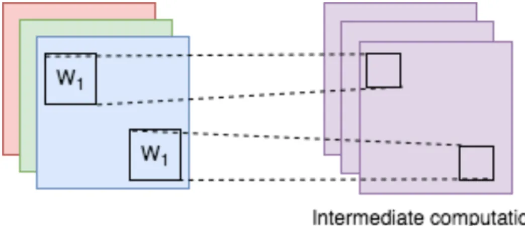
The second important property is parameter sharing. The weights with which the input layers nodes are convolved remains the same for each output node belonging to the same kernel. Figure 2.2 shows different patches of one channel being convolved with the same kernel W1 to produce one feature map. Firstly, this enforces that any given kernel is

looking for one kind of pattern. When combined with non-linearity and deeper architectures this adds immense power to the network. By forcing all the weights to be the same for each input-output neuron pair, the number of parameters is reduced drastically thus further reducing any chance of overfitting.

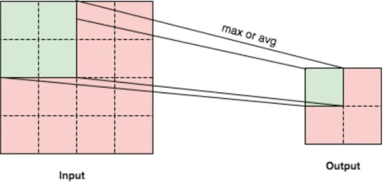
Figure 2.3 Pooling operations

The first two properties give the network the capability of translational equivariance i.e., if the input is moved slightly then the output of the network also moves by the same amount. The third property of the network adds translational invariance in the network. Pooling operations break the output of the convolution layer into multiple segments and

perform some simple operation on each segment. This is usually a maxpool operation where the maximum of all values in the segment is taken as the output. This allows the input features to move slightly spatially yet produce the same output. The working of a Pooling layer is explained in Fig. 2.3, where a max/avg operation is applied on 4 cells of one layer to produce one cell in the next layer. In our previous work [27], we used RNNs to model the temporal structure of the EEG data, however in a recent work [39], the RNN has been replaced by a CNN. There are certain advantages to this choice, as RNNs are in general hard to train whereas CNNs train faster. Using a CNN, we will be able to learn the required features automatically instead of hand-engineering them.

2.2.3

2D Convolution

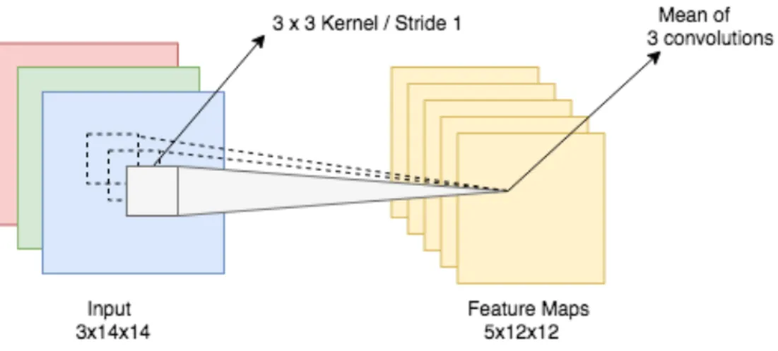
In a 2D Convolution layer, the input to the layer is a 3D tensor containing several channels of 2D “images”. A kernel is used to extract features from the input tensor, and this kernel is learned through backpropagation. A bias is added to the output of the kernel and an optional non-linearity is applied.

Each kernel moves over each pixel of the image and an elementwise multiplication and summation is performed. The sum for each pixel from each channel of the input image is averaged or summed. The formula for a 2D convolution is given below. Assume that the input is denoted as I, output as O, r and c are the indices for the output, m is the number of

input channels, b is the index for the feature map and HW is the size of the kernel and 𝜎 is the activation function, typically ReLU.

𝑂_𝑏𝑟𝑐 _{= 𝜎 𝑏𝑖𝑎𝑠} 𝑏+ 1 𝑚 𝑤𝑒𝑖𝑔ℎ𝑡𝑏𝑚 ℎ𝑤 _𝐼 𝑚 (𝑟+ℎ)(𝑐+𝑤) 𝑊 −1 𝑤=0 𝐻−1 ℎ= 0 𝑚

2.2.4

3D Convolution

In a 2D convolution, only 2 dimensions can be captured. In vision, this would-be height and width of the input feature map/image. Although an image may contain up to four channels, it is not counted into the dimension of the convolution and is simply referred to as a 2D convolution. For this project, 2D convolution happens over electrodes and time. However, there are many applications where the input is 3 dimensional (+ additional channel information). For e.g., as described in section 3.3, we perform AEP, a technique that projects hemispherical arrangement of electrodes on the brain onto an 8x8 grid, similar to how the globe is projected onto a 2D map. To deal with this case, we can simply extend the idea of 2D convolution to 3 dimensions. Following the same notation as in the previous section, and introducing D as the depth of the kernel, z as the depth index for the output, we have,

𝑂_𝑏𝑟𝑐𝑧 _{= 𝜎 𝑏𝑖𝑎𝑠} 𝑏+ 1 𝑚 𝑤𝑒𝑖𝑔ℎ𝑡𝑏𝑚 ℎ𝑤𝑑 _𝐼 𝑚 (𝑟+ℎ)(𝑐+𝑤)(𝑧+𝑑) 𝐷−1 𝑑=0 𝑊 −1 𝑤=0 𝐻−1 ℎ= 0 𝑚

Similar to the 2D conv, the training of the 3D conv kernels happens through backpropagation.

2.2.5

Batch Normalization

It is very common to normalize the input to a training mechanism. This improves the training speed by placing all the attributes roughly in the same scale. This in turn skews the error function into a more hyper spherical shape leading to faster convergence. Recently, BatchNorm [40] has been proposed as a method of speeding up training by controlling internal covariate shift. [40] describes internal covariate shift as the change in the distribution of network activation due to the change in network parameters during training. This problem is solved by fixing the input distribution to the particular layer. More specifically, the output of intermediate layers is normalized to have mean 0 and variance 1. To allow the network to choose a different mean and variance, two learnable parameters – g and b – are introduced. The equations relating to batch normalization are mentioned below.

𝜇_Β = 1 𝑚 𝑥𝑖 𝑚 𝑖 = 1 𝜎_ℬ2 ₌ 1 𝑚 (𝑥𝑖− 𝜇ℬ) 2 𝑚 𝑖 = 0 𝑥_𝚤 = 𝑥𝑖− 𝜇ℬ 𝜎_ℬ2 _+𝑒 𝑦_𝑖 = 𝛾𝑥_𝚤 + 𝛽

BatchNorm has an unexpected side-effect of acting as a regularizer. As the training progresses, the mean and variance used keeps changing and is not deterministic for a given

training sample. This introduction of noise is a form of regularization and was found to be advantageous for generalization of the network.

2.3

Interpretability

Neuroscience research is often concerned with determining which brain regions are responsible for which cognitive processes. The analysis could provide answers to non-invasive questions but also to questions like which part of the brain should the surgeon cut without damaging brain function. Therefore, interpretability is of key importance.

Typically, linear models are used as they are often highly interpretable using the weights learned by the model. However, they are only discriminative models and there is no reason to assume that the weights exactly represent the nature of one class against the other for any purpose other than discrimination. Particularly, there could be several channels containing signal that is not of interest, possibly having high weights in the learned linear model. As an extreme case, if only classifier weights were used to determine which parts of the brain to remove there could be severe consequences.

While the solution for this problem is summarized in the next section and described in detail in [31], we are faced with another issue entirely. Neural networks have become much better in the last decade, yet remain stubbornly uninterpretable. One important reason is that the information is captured in the weights of the network, with few ways to extract the knowledge. In the coming chapters, we propose a linear CNN that outperforms existing methods and show a hack to distill the knowledge from the network into a logistic regression

model exactly. Thus, we obtain a linear network which can be interpreted in the same way as described in the next section.

2.3.1

Converting backward models to forward models

Haufe et al. [31] refers to the methods that use data to extract neural information from data as backward models. In contrast, what we require is a forward model, one that can explain how the data was generated in the first place. The backward model contains nonzero weights representing activations that are irrelevant. Hence, a logistic regression model that is trained to discriminate P300 vs non-P300 data is the backward model and it has to be converted into a forward model, which is the activation pattern that the model believes has generated the data. Under certain assumptions, the recipe for this conversion is rather simple and is described in detail in [31]. Let the discriminator be described as,

𝑊′_{𝑥(𝑛) = 𝑦(𝑛)}

The activation pattern A, can be obtained using the following formula,

𝐴= Σ_𝑥𝑊 Σ_𝑦−1

where, Σ_𝑥 = 𝔼𝑥(𝑛)𝑥(𝑛)′ _{and Σ} 𝑦

Chapter 3

Methods:Pre-processing and Classification

This chapter discusses the dataset used for evaluating the classifiers, data-pre-processing techniques and proposed ideas for improving P300 classification.

3.1

P300 Dataset

The dataset used in this experiment is BCI Competition III Dataset II first described in [41]. The dataset is a record of P300 evoked potentials recorded with BCI2000 using the method described in [9]. In the original contest, the goal was to predict the correct character. The user was presented with a 6x6 grid of characters as described in section 1.2. The rows and columns were successively and randomly intensified at a rate of 5.7Hz. Two out of 12 intensifications of rows or columns contained the character the user wanted to communicate and the rest did not. A set of 64 electrodes were placed as described in [42], shown in Figure 3.1.

Figure 3.1 Location of the electrodes on the scalp [49]

The recorded signals were bandpass filtered from 0.1-60Hz and digitized at 240Hz from two subjects (henceforth addressed as Subject A and Subject B). The experiment consisted of several runs and in each run the subject was asked to focus on a certain sequence of letters. For each character in a run, the whole display was first intensified for 2.5s and then each row and column was randomly intensified for 100ms thus resulting in 12 trials. Further, for each character this process was repeated 15 times. The idea here is that since the trials are noisy, an averaging process would be required. Thus, there are 180 trials per character. With 85 characters in the experiment, each subject effectively gives us 15300

P300 trials. Each subject repeated this process once again at a different time, and this data is provided by the authors as a test dataset. The results for the test dataset were made public after the competition was complete.

3.2

Objective

In the original competition, the task was to use labeled training data to predict the character series in a test set. The competitors had to deliver a total of 4 character vectors, each 100 characters long. Each deliverable belongs to either Subject A or Subject B and was predicted using either all 15 sets of intensifications or just 5 sets of intensifications. To serve as a reminder, this was done to remove noise in the data. However, for the purposes of our work, we use these signals differently.

We have about 15300 independent raw P300 signals (12 row/col x 15 intensifications x 85 characters). Of these, 12750 signals correspond to “non-target” category – signals where the P300 is not expected, as only two of 12 intensifications contain the particular character – and the rest correspond to “target” category, where P300 is expected. Each of these trials is 64x156 dimensional input (64 channels and 156 time points). The goal is to build a robust classifier that works well for the classification of raw P300. The next steps describe the pre-processing techniques used in this work.

3.3

Data pre-processing

The dataset is presented in a continuous format, thus epoching was performed by selecting the signals between 0ms and 650ms after each event (intensification of a

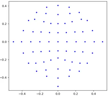
row/column). The data was further bandpass-filtered between 0.1-20Hz. While the baselines (LDA) do not use any temporal or spatial structure of the data, the more advanced techniques use only the temporal structure in the data but ignore the spatial organization of the electrodes. For this purpose, not much pre-processing is required. However, we have also explored an architecture capable of exploiting spatial information for which the relative locations of the electrodes must be captured in the data. EEG recording devices are arranged over a hemispherical manifold in 3D space i.e. the brain. This is projected onto 2D using a 3D to 2D projection technique called the azimuthal equidistant project (AEP) [43]. This is similar to how a world map is constructed from a globe. We assume that the center point of the projection is the north pole. Therefore, the angle made with the center point is the polar angle, and the circular polar angle is the angle subtended by the electrode and the back of the head. Ideally, we would like to preserve relative distances between all the electrodes, but this is not possible in 2D. AEP preserves the relative distance between different electrodes and the center point. Once this 2D projection is created, we perform a cubic spline interpolation to get an 8x8 grid. Larger or smaller sizes can be opted, but from our previous work in [27], we found that any increase in size doesn’t offer better results and a decrease increased the smoothness of the projection. Given an input signal, this projection must be performed for the values of the electrodes at every single time point. This converts the data from a 2D format to a 3D format. An example of AEP on EEG and an interpolation forming an 8x8 grid is shown in Figure 3.2.

a) AEP performed for selected dataset

b) Interpolated locations forming 8x8 grid

3.4

Popular Architectures

3.4.1

EEGNet

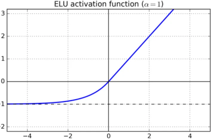
The EEGNet architecture a is simple fully convolutional network which performed well in our experiments. According to [2], this is the model that performed well over four different experiments and was proposed as a generic model for BCIs. The architecture of the model is expressed in Table 1. The model uses an activation function called ELU with _𝛼=1 which is shown in Figure 3.2. It is trained using Adam and optimizes the cross-entropy criterion and was run for 500 epochs.

Table 3.1 Architecture of EEGNet

Layer Input (CT) Operation Output

1 C x T 16 x Conv1D(Cx1) 16 x 1 x T 16 x 1 x T BatchNorm 16 x 1 x T 16 x 1 x T Reshape 1 x 16 x T 1 x 16 x T Dropout (0.25) 1 x 16 x T 2 1 x 16 x T 4 x Conv2D (2 x 32) 4 x 16 x T 4 x 16 x T BatchNorm 4 x 16 x T 4 x 16 x T Maxpool2D (2, 4) 4 x 8 x T/4 4 x 8 x T/4 Dropout (0.25) 4 x 8 x T/4 3 4 x 8 x T/4 4 x Conv2D (8x4) 4 x 8 x T/4 4 x 8 x T/4 BatchNorm 4 x 8 x T/4 4 x 8 x T/4 Maxpool2D (2, 4) 4 x 4 x T/16 4 x 4 x T/16 Dropout (0.25) 4 x 4 x T/16 4 4 x 4 x T/16 Sigmoid 1

Figure 3.3 Exponential Linear Unit with formula

3.4.2

CecottiNet

The two most successful networks proposed by [4] were CNN-1 and MCNN-3, however MCNN-3 is an ensemble of 3 CNN-1’s. Since ensembling is a technique that helps reduce errors due to variance, it can be used for most neural networks to obtain small performance gains. This was the case in [4] where the performance difference between MCNN-3 and CNN-1 is very small. We refer to CNN-1 as CecottiNet for clarity. CecottiNet was tested on BCI Competition III Dataset II, which is the same dataset used in this work. The model proposed by them is presented succinctly in Table 2. The network is shown in Figure 3.3.

Table 3.2 Architecture of CecottiNet

Layer Input Operation Output

1 C x T 10 x Conv1D (1, C) 10 x 1 x T 2 10 x 1 x T Reshape 1 x 10 x T 3 1 x 10 x T 5 x Conv2D (1, 13) / Stride = 13 5 x 10 x 6 4 5 x 10 x 6 Dense (100) 100 5 100 Softmax 2 𝑓(𝛼,𝑥) = {𝛼(𝑒 𝑥_{−1), 𝑥< 0} 𝑥, 𝑥 ≥0

Cecotti et al. [4] proposed various additional implementational details including data-normalization, varying learning rates for different layers, relationship between the number of layers, specific activations functions. They proposed that the input to the network be sampled at 120Hz and z-scored according to the following formula.

𝐼_𝑖𝑗= 𝐼𝑖,𝑗− 𝐼𝑖

𝜎_𝑖

where, Iij is the final signal value, Ii,j is the original value and 𝐼$ is the mean value, 𝜎$ is the

standard deviation. They also proposed that layers L₁ and L2 use the learning rate

𝛾 = 2𝜆

𝑛 𝑙,𝑚, 0 _𝑁

shared 𝑛 𝑙,𝑚,𝑖 𝑁input

and the learning rate used by layers L3 and L4 is,

𝛾 = 𝜆

𝑛 𝑙,𝑚,𝑖 _𝑁

input

Here, 𝜆 is some constant, 𝑛(𝑙, 𝑚, 𝑖) denotes the ith _{value in the m}th _{feature map of the outputs} of the lth _{layer. 𝑛 𝑙,𝑚,𝑖}

𝑁input is the number of inputs to 𝑛 𝑙, 𝑚, 𝑖 and 𝑛 𝑙,𝑚, 0 𝑁shared refers to the

number of neurons that share the same set of weights.

3.5

Architectural Tests

The following subsections describe each change performed on the EEGNet network.

3.5.1

Square kernels

The most commonly used kernel shape in deep learning methods in computer vision tasks are of 3x3 shape. This is because this is the smallest kernel size that captures the notion

of height and width. However, EEGNet makes the unusual choice of rectangular kernels. We set the kernel size in all layers after the first to be 3x3, leading the number of outputs in the penultimate layer to increase by 4 times.

3.5.2

Linear activation function

In studies [44], it has been shown that ReLU activation performs best in the context of NLP and Computer Vision. Previous work [34], [35], [36] uses similar non-linear activation functions in accordance with these studies. However, the leading models used for P300 classification. [25][26] use LDA based approaches. It is known that LDA provides a linear separating boundary. To test whether linear networks could be better, we switched out all ELU activation units and replaced with linear activation functions. However, this doesn’t completely linearize the network. Since the network becomes simpler, we also removed dropout while training as the chances of overfitting are reduced.

3.5.3

Spatio-temporal kernel

In Deep learning networks proposed to tackle EEG-based BCI problems generally do not combine spatial and temporal filters. It is common to first dissolve all spatial information using a spatial filter and then perform temporal convolutions as done in both EEGNet [2] and Shallow/Deep ConvNet [36]. Even in our previous work [27], we convolved spatially first and then fed the transformed timeseries data to an LSTM to learn temporal patterns. However, in recent work by [45], it was proposed that by looking at both spatial and temporal information using a spatio-temporal kernel can help the network work better. Therefore, the first layer kernel was made into a spatio-temporal kernel of size (3, C). The value 3 was chosen by cross-validation.

3.5.4

Large temporal convolutions

The first layer is fed data without spatial structure and filter that covers all electrodes is used, therefore most variation is captured in the temporal structure of the data. We emphasize this in the network by making it look at longer segments of the timeseries, by simply using kernels that are wider along the temporal axis i.e. instead of (8, 4) kernels, we used (4, 10) kernels.

3.5.5

Network size

EEGNet places an emphasis on keeping the number of parameters low to reduce training time, and to keep the network simple. However, we can make the network bigger without adding much complexity, as we have reduced the complexity of the model by using linear units. In the comparison, we will see the effect of using larger network size alone (non-linear network) to see the effects of this change individually. We used 8 kernels in both the second and third layer.

3.5.6

Average pooling

The common notion is that max-pooling is better as a design choice. This is because the idea behind the pooling operation is that once we have extracted features from the previous layer, the exact location of the features is not as important. The max-pool layer accepts only the highest activation from a fixed block, because this maximum value is obtained from highest similarity to the kernel. However, after performing linear activation, the only network element that keeps the network non-linear is this max-pooling operation.

As discussed later, it is possible to distill the knowledge of a linear deep network into a simple logistic regression model. This will enhance interpretability. To allow this, we replaced max-pooling with avg-pooling hoping for minimal impact on performance. Contrary to our assumptions, the avg-pooling works better.

3.5.7

Using 3D data

Section 3.2 described a technique to preserve spatial information in the EEG data by projecting the data onto a 2D plane. In contrast to the standard approaches, this method allows us to carry spatial information forward. This method was previously adopted in [35]. To check whether this is of significance, we used 3x3 kernels in the first layer, but fed projected data. The rest of the network was modified minimally as presented below.

Each change from sections 3.5.2 to section 3.5.6 was performed incrementally to check additional improvement. The final model based on the results contained proposals defined in sections 3.5.2 through 3.5.6. This model is henceforth termed as EEGNet+ and is coincidentally, completely linear except for the softmax layer.

3.6

Knowledge distillation

A problem with neural networks is that they act like black boxes. It is hard to explain what they have learnt. Some techniques like DeepLIFT [46] have been created to allow interpretation. However, since EEGNet+ is linear, we can take a simpler approach. The only issue with visualizing the patterns learned by EEGNet is that the effective weight corresponding to each input feature is hidden in the weights and biases of the different layers. For a fully connected network, we can simple represent each layer as a weight matrix and

simply perform matrix multiplication. But to do this for networks with convolutional layers, we have to construct Toeplitz matrices out from the inputs to each layer (rather than the weights themselves). This is cumbersome to do and we therefore present a much simpler method to distill the knowledge. We can learn a logistic regression model that is equivalent to a trained EEGNet+ and produces the exact same output for a given input. The general form of a logistic regression looks like,

𝑦= 𝜎 𝑤_𝑖

𝑛 𝑖=0

𝑥_𝑖+𝑏

where we are the weights associated with feature i, and b is the bias. We are now required to

infer these weights wi from those that are in the trained network. This can be easily done by

providing specific inputs to the neural network (without softmax). The simple algorithm is presented below.

Algorithm LearnEquivalentLRModel

Input: Trained EEGNet+ model without before applying softmax, M

Number of input features, f

Create a logistic regression model L with weights w1, w2 … wf, and bias b.

Set 𝑏=𝑀(0)

for 𝑖= 1→ 𝑓 do

I = input array of size f filled with zeros except location i, which is set as 1.

𝑤$ = 𝑀 𝐼

return L

This method works by first supplying an all 0 input to the network, which yields the bias. Thereafter, we supply inputs with just one feature having a value of 1 and the others as 0. If the kth feature is 1, then the value of the network is equal to wk+b.

Chapter 3, in part, was submitted to BCI Meeting 2018, Ravindran, Sriram; de Sa, Virginia R. The thesis author was the primary investigator of this material.

Chapter 4

Experimentation, results and discussion

4.1

Experimental Setup

The study was performed on EEGNet on a competition dataset, the BCI Competition III Dataset II. The goal of the competition was to find out the characters that the subject was asked to spell in the test dataset. The dataset is provided as a continuous signal along with the character the user was supposed to be thinking of at the time. Using this, we chopped the signal into trials. We picked up data between 0-650ms of each stimulus. Since the sampling frequency is 240Hz and the number of channels are 64, the size of each trial is 64x156. The corresponding output for each trial is binary, 1 corresponds to target signals (P300) and 0 to non-target signals (no P300). For each subject during training, we have 15300 training trials. Of these only, 2550 are target signals. We first shuffled the data intra-class and then split the data into 5 parts i.e. we took 80% data from each class for training and 20% data for validation. Since the data is heavily imbalanced in favour of non-target class, we replicated the information in the target class 5 times for both training and validation data.

We trained the network using cross-entropy loss function with Adam optimizer. The parameters of the Adam optimizer were the same as described in the original paper [50]. This is because Adam is an improvement over both Adagrad and RMSprop and worked well for our needs. We used a mini-batch size of 200 and did not use dropout. Our network is quite simple, and does not overfit that easily. We didn’t use any regularization for the same reason. We ran the network for 50 epochs, and recorded validation performance at each epoch, storing the model if it was better than the previous best. We finally picked the model that had highest performance within these 50 epochs. We found that the network always obtained its best performance around 15-20 epoch and degraded thereafter. The performance metric used was f-measure, as it tries to balance both precision and recall.

Usually, the training and testing data are assumed to be drawn from the same distribution, however this is not the case with the selected dataset. The test dataset was recorded on different day from the training dataset, and early experiments revealed that improved validation performance did not give improved test performance. Therefore, we used Subject A’s test data (after training with a single fold) to make decisions as to whether a modification was helpful or not. Once that was deciced, the average test performance from all folds was reported. One could argue that we overfit to Subject A’s test data by modifying the architecture; therefore, the results from Subject A are only partly reliable for this reason. However, Subject B’s test data was never used and yet Subject B’s results’ improvements mirror those of Subject A. In addition, linear CecottiNet works better too, despite not looking at any test data. Any decisions about what dimensionality to use for LDA by looking at our test-set performance would also be subject to the same overfitting criticism.

4.2

Results

Normally, the approach is to divide each trial into 5 or 10 time windows, average within each window and use it as an input to the classifier. However, we use the full signal without making any modifications. For models that expect 3D inputs we simply performed AEP. For comparison, we also ran the tests on 10, 20 and 30-window Shrinkage LDA. The algorithm uses the automated shrinkage algorithm as proposed by Schaefer and Strimmer [47]. In the following tables, EEGNet refers to model in section 3.5.1 only, 3D-EEGNet refers to the model in 3.5.7 only, v2 refers to section 3.5.2, v3 for section 3.5.3, v4 for section 3.5.4, v5 for section 3.5.5 and EEGNet+ for section 3.5.6. All changes from 3.5.2 to 3.5.6 were performed incrementally.

Table 4.1 Performance measures for various classifiers for Subject A (details in section 4.2)

Model Subject A

Accuracy AUC Precision Recall F-measure

Shrinkage-LDA (10 windows) 0.697 0.744 0.307 0.646 0.416 Shrinkage-LDA (20 windows) 0.711 0.75 0.318 0.641 0.426 Shrinkage-LDA (30 windows) 0.715 0.750 0.32 0.63 0.424 EEGNet 3x3 0.64 0.709 0.267 0.678 0.383 3D-EEGNet 0.666 0.738 0.29 0.69 0.408 Original EEGNet 0.643 0.709 0.27 0.658 0.381 EEGNet v2 0.659 0.725 0.283 0.674 0.398 EEGNet v3 0.676 0.733 0.292 0.682 0.406 EEGNet v4 0.678 0.744 0.297 0.682 0.414 EEGNet v5 0.685 0.767 0.311 0.725 0.435 EEGNet+ 0.716 0.773 0.33 0.684 0.445

Table 4.2 Performance measures for various classifiers for Subject B (details in section 4.2)

Model Subject B

Accuracy AUC Precision Recall F-measure

Shrinkage-LDA (10 windows) 0.739 0.792 0.357 0.702 0.47 Shrinkage-LDA (20 windows) 0.759 0.804 0.38 0.701 0.493 Shrinkage-LDA (30 windows) 0.766 0.806 0.388 0.699 0.499 EEGNet 3x3 0.685 0.751 0.303 0.688 0.421 3D-EEGNet 0.674 0.729 0.29 0.6644 0.404 Original EEGNet 0.699 0.759 0.315 0.682 0.43 EEGNet v2 0.728 0.772 0.338 0.658 0.447 EEGNet v3 0.712 0.783 0.333 0.716 0.454 EEGNet v4 0.729 0.792 0.348 0.705 0.466 EEGNet v5 0.765 0.796 0.383 0.653 0.481 EEGNet+ 0.767 0.828 0.393 0.74 0.513

In order to show that these measures are indeed a good choice for P300 tasks, we have shown the improvement in CecottiNet. We did not implement CecottiNet in its full spirit; they used SGD with momentum, we used the superior Adam. We did not use different learning rate for different layers, therefore we are unable to replicate the results of the paper. However, our goal is to show that using linear activation helps, therefore, we only expect to show a relative improvement in performance.

Table 4.3 Performance measures for CecottiNet

Model Subject A Subject B

AUC Accuracy F-measure AUC Accuracy F-measure

CecottiNet (Original) 0.659 0.635 0.348 0.749 0.694 0.423 CecottiNet (Linear) 0.718 0.665 0.39 0.781 0.74 0.462

4.3

Visualization

To produce these plots, we extracted the weights for each data point in trial using the algorithm described in the section 3.6. Then we used the method described in section 2.3.1. using the test data, to produce the following visualization for both subject A and B using both EEGNet+ and Shrinkage LDA. To produce these plots, we used the plot_topomap from mne package for python. The vmax was set to 30000 and vmin to -30000. The following plots are to be seen left to right, top to bottom, and they represent the activation pattern from 0 to 650ms after stimulus. EEGNet+ actually produces 156 plots i.e. the number of timepoints per trial. For clarity, we have only sampled a plot once every 10 timepoints (corresponds to ~42ms).

Figure 4.2 The activation patterns as learned by EEGNet+ for Subject B

Figure 4.4 Activation patterns learned by Shrinkage-LDA for Subject B with 10 buckets

As we can see, both EEGNet+ and LDA learn the patterns that look similar to the P300 – an increasing and then decreasing activation around the central area of the brain. Both models show activations in the frontal area of the brain, except for LDA performed on Subject B. Also, EEGNet+ produces more consistent plots between the two subjects than LDA. Although all plots are standardized by setting a maximum and minimum value corresponding to red and blue, the activations in Subject B seems to be very extreme when the LDA weights are used, nevertheless following the P300 pattern.

Chapter 4, in part, was submitted to BCI Meeting 2018, Ravindran, Sriram; de Sa, Virginia R. The thesis author was the primary investigator of this material.

Chapter 5

Conclusion and Future Work

In this work, we performed a study of an existing neural network on the task of single trial P300 classification and demonstrated a technique to visualize the activation patterns learned by it. In comparison to previous neural network methods, this method is linear in nature which allows it to be interpreted. We also demonstrated that some choices that helped improve EEGNet, also improved CecottiNet. Architectural choices and hyperparameter selection are a common issue faced by neural network researchers. There exists a methodical way to test multiple hyperparameters but no guidelines for architecture selection. We conclude that it might interesting for researchers to adopt some choices provided in this work in order to enhance performance and improve interpretability.

From our study of the network, we found that projecting EEG channel data onto an “image” spatial structure of EEG did not provide significant benefits. This may not be the best way to preserve spatial structure of EEG data. The network overfits quite rapidly despite

regularization indicating that a non-linear model is too complex for modelling EEG data, at least standard-sized EEG datasets. Therefore, we proposed the use of linear activation units. CecottiNet also improved in performance when used with linear neurons.

We confirmed the effectiveness of using spatio-temporal convolutions in the initial layer. Other models being used for this purpose convolve over purely electrodes or time. We believe that allowing the kernels to look forward in time, although in limited capacity, improves performance up to an extent. This is consistent with our results from an earlier paper [26] where 3D-CNN showed improved performance.

The use of square 3x3 kernels sharply decreased the performance. In the case of 2D data, rectangular kernels do not make much sense as adjacent rows of data (electrodes) do not correspond to data that are spatially closer to one another. However, it allows us to learn relationships between different electrodes if there is any. More importantly, we can infer that having large kernel sizes over the temporal axis is beneficial as it allows the network to see more variation. The same idea was extended to the third layer of EEGNet, where the use of short-wide kernels instead of tall-narrow kernels yielded an increase in performance.

A sharp improvement arose from the use of average pooling instead of maximum pooling. Max-pooling is very popular in computer vision applications; however, it makes the network non-linear despite the use of linear activation units. Using average pooling makes the network more linear – fully linear when used in tandem with linear activation in our case. Common methods used in the classification of EEG data utilize linear models very successfully. Perhaps linear models are better suited for EEG decoding with limited data.

We tested the effectiveness of mapping the spatial structure of EEG to an image. Unfortunately, we failed to improve performance by introducing spatial information in this manner. However, we did not extensively work on this area. In our previous work, we achieved good results with models that used spatial structure in this way. Therefore, more work is needed in this area.

We transferred the knowledge from the EEGNet+ into a logistic regression model and interpreted the weights as dictated by [31]. On visualizing the learned activation patterns, we noticed that the network correctly learns the expected form of the P300. It shows increasing activation for both Subjects at the centre of the brain – near the Cu electrode – from around 350ms to 400ms after event and drops thereafter. We also noticed that the network indicates significant activity in the prefrontal cortex of the brain which is not usually associated with the P300. Whether this is a drawback of the model or an unknown aspect of P300 can be determined with further study only.

As a future direction, we propose the use of this network for various other EEG applications/datasets to determine whether these results are valid for other types of ERPs. The performance, while better, is still not good enough to create reliable spellers that could function entirely using only single-trial EEG. Therefore, it needs to be improved further.

References

[1]Kingman, Diederik P and Ba, Jimmy Lei. Adam: A method for stochastic optimization. arXiv preprint arXiv:1412.6980, 2014.

[2] Vernon J. Lawhern, Amelia J. Solon, Nicholas R. Waytowich, Stephen M. Gordon, Chou P. Hung: “EEGNet: A Compact Convolutional Network for EEG-based Brain-Computer Interfaces”, arXiv:1611.08024, 2016

[3] Robin Tibor Schirrmeister, Jost Tobias Springenberg, Lukas Dominique Josef Fiederer, Martin Glasstetter, Katharina Eggensperger, Michael Tangermann, Frank Hutter, Wolfram Burgard: “Deep learning with convolutional neural networks for EEG decoding and visualization”, arXiv: 1703.05051, 2017

[4] Cecotti, H., & Graser, A. (2011). Convolutional Neural Networks for P300 Detection with Application to Brain-Computer Interfaces. IEEE Transactions on Pattern Analysis and Machine Intelligence, 33(3), 433–445. https://doi.org/10.1109/tpami.2010.125 [5] Vespa, Paul M.; Nenov, Val; Nuwer, Marc R. (1999). "Continuous EEG Monitoring in

the Intensive Care Unit: Early Findings and Clinical Efficacy". Journal of Clinical Neurophysiology. 16 (1): 1–13. doi:10.1097/00004691-199901000-00001 PMID 1008 2088.

[6] Hämäläinen, Matti; Hari, Riitta; Ilmoniemi, Risto J.; Knuutila, Jukka; Lounasmaa, Olli V. (1993). "Magnetoencephalography-theory, instrumentation, and applications to noninvasive studies of the working human brain". Reviews of Modern Physics. 65 (2): 413–97. Bibcode:1993RvMP...65..413H. doi:10.1103/RevModPhys.65.413

[7] Murphy, Kieran J.; Brunberg, James A. (1997). "Adult claustrophobia, anxiety and sedation in MRI". Magnetic Resonance Imaging. 15 (1): 51–4. doi:10.1016/S0730-725X(96)00351-7. PMID 9084025

[8] Srinivasan, Ramesh (1999)."Methods to improve the Spatial Resolution of EEG" Int. J. Bioelectromagn. (1): 102–11

[9] Farwell, L. A., & Donchin, E. (1988). Talking off the top of your head: toward a mental prosthesis utilizing event-related brain potentials. Electroencephalography and Clinical Neurophysiology, 70(6), 510–523. https://doi.org/10.1016/0013-4694(88)90149-6 [10] Herrmann, C. S. (2001). Human EEG responses to 1-100Hz flicker: resonance

phenomena in visual cortex and their potential correlation to cognitive phenomena. Experimental Brain Research, 137(3–4), 346–353. https://doi.org/10.1007/s0022101 00682

[11] Neuper, C. and Pfurtscheller, G., Event-related dynamics of cortical rhythms:frequency specific features and functional correlates, Int. J. Psychophysiol., 43, 41, 2001.

[12] Birbaumer N., Kubler A., Ghanayim N., Hinterberger T., Perelmouter J., Kaiser J., Iversen I., Kotchoubey B., Neumann N., Flor H. (2000). The thought translation device (TTD) for completely paralyzed patients. IEEE Trans. Rehabil. Eng. 8, 190–193. [13] Fazel-Rezai, R., Allison, B. Z., Guger, C., Sellers, E. W., Kleih, S. C., & Kübler, A.

(2012). P300 brain computer interface: current challenges and emerging trends. Frontiers in Neuroengineering, 5. https://doi.org/10.3389/fneng.2012.00014.

[14] Picton, T. W. (1992). The P300 Wave of the Human Event-Related Potential. Journal of Clinical Neurophysiology, 9(4), 456–479. https://doi.org/10.1097/00004691-199210000-00002

[15] Birbaumer, N., McFarland, D.J., Pfurtscheller, G., Vaughan, T.M., & Wolpaw, J.R. (2002). Pii: S1388-2457(02)00057-3.

[16] Fazel-Rezai, R., & Abhari, K. (2009). A region-based P300 speller for brain-computer interface. Canadian Journal of Electrical and Computer Engineering, 34(3), 81–85. https://doi.org/10.1109/cjece.2009.5443854

[17] Citi, L., Poli, R., Cinel, C., & Sepulveda, F. (2008). P300-Based BCI Mouse With Genetically-Optimized Analogue Control. IEEE Transactions on Neural Systems and Rehabilitation Engineering, 16(1), 51–61. https://doi.org/10.1109/tnsre.2007.913184 [18] Jun, Y. B., Lee, K. J., & Park, C. H. (2010). Fuzzy soft set theory applied to

BCK/BCI-algebras. Computers & Mathematics with Applications, 59(9), 3180–3192. https://doi.org/10.1016/j.camwa.2010.03.004