IM-NET: Learning implicit fields for generative shape modeling

(1)

IM-NET: Learning Implicit Fields for

Generative Shape Modeling

by

Zhiqin Chen

B.Sc., Shanghai Jiao Tong University, 2017

Thesis Submitted in Partial Fulfillment of the Requirements for the Degree of

Master of Science

in the

School of Computing Science Faculty of Applied Sciences

c

Zhiqin Chen 2019

SIMON FRASER UNIVERSITY Summer 2019

Copyright in this work rests with the author. Please ensure that any reproduction or re-use is done in accordance with the relevant national copyright legislation.

(2)

Approval

Name: Zhiqin Chen

Degree: Master of Science (Computing Science)

Title: IM-NET: Learning Implicit Fields for Generative Shape Modeling

Examining Committee: Chair: Manolis Savva Assistant Professor Hao Zhang Senior Supervisor Professor Daniel Cohen-Or Supervisor Professor

Department of Computer Science Tel Aviv University

Vladimir Kim

External Examiner Senior Research Scientist Adobe Research

(3)

Abstract

We advocate the use of implicit fields for learning generative models of shapes and intro-duce an implicit field decoder, called IM-NET, for shape generation, aimed at improving the visual quality of the generated shapes. An implicit field assigns a value to each point in 3D space, so that a shape can be extracted as an iso-surface. IM-NET is trained to perform this assignment by means of a binary classifier. Specifically, it takes a point coordinate, along with a feature vector encoding a shape, and outputs a value which indicates whether the point is outside the shape or not. By replacing conventional decoders by our implicit decoder for representation learning (via IM-AE) and shape generation (via IM-GAN), we demonstrate superior results for tasks such as generative shape modeling, interpolation, and single-view 3D reconstruction, particularly in terms of visual quality.

Keywords: implicit field; shape generation; representation learning; generative model; single-view 3D reconstruction

(4)

Acknowledgements

I would like to thank my supervisor, Dr. Hao Zhang, for his enormous effort and insights put into this project, and for pushing me to eventually publish this work on a top conference.

I would also like to thank Matt Fisher and Daniel Cohen-Or for their invaluable com-ments, Kangxue Yin and Ali Mahdavi-Amiri for the proofreading, and all my friends who have discussed with me about this project and shared with me their opinions.

Special thanks to Jon Liu, who have lent me his computer in the lab when I was in urgent need of GPUs.

Last but not least, I thank my parents for their love and support throughout the years. The research is supported by NSERC and an Adobe gift fund.

(5)

List of Tables

Table 5.1 3D reconstruction errors. CNN and IM represent CNN-AE and IM-AE, respectively, with 64 and 256 indicating sampling resolutions. The mean is taken over the first 100 shapes in each tested category. MSE is multiplied by 103, IoU by 102, and CD by 104. LFD is rounded to integers. Better-performing numbers are shown in boldface. . . 18 Table 5.2 Quantitative evaluation of 3D shape generation. LFD is rounded to

integers. See texts for explanation of the metrics. . . 20 Table 5.3 Quantitative evaluation for 2D shape generation. Oracle is the results

obtained by using the training set as the sample set. The metrics with-out suffix “-nb” are evaluated using binarized images. PWE and IS are the higher the better. The better results in each subgroup (latent-GAN, VAE, WGAN) are bolded, and the best results over all models are underlined. . . 22 Table 5.4 Quantitative evaluation for SVR using LFD. The means are taken over

the first 100 shapes in the testing set for each category and rounded to integers. AtlasNet25 is AtlasNet with 25 patches (28,900 mesh vertices in total) and AtlasNetO (7,446 vertices) is with one sphere. IM-SVR and HSP were both reconstructed at 2563 resolution. . . 23 Table 5.5 Quantitative evaluation for SVR using CD. The means are taken over

the first 100 shapes in the testing set for each category. CD is multiplied by 104. . . 23

(8)

List of Figures

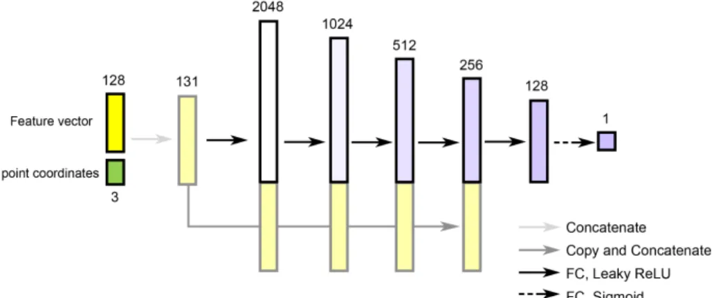
Figure 1.1 3D shapes generated by IM-GAN, ourimplicit fieldgenerative adver-sarial network, which was trained on 643 voxelized shapes for chair category and 1283 voxelized shapes for car and plane category. The output shapes are sampled at 5123 resolution and rendered after Marching Cubes. . . 2 Figure 1.2 Network structure of our implicit decoder, IM-NET. The network

takes as input a feature vector extracted by a shape encoder, as well as a 3D or 2D point coordinate, and it returns a value indicating the inside/outside status of the point relative to the shape. The encoder can be a CNN or use PointNET [36], depending on the application. 2 Figure 1.3 CNN-based decoder vs. our implicit decoder. We trained two

au-toencoders with CNN decoder (AE_CNN) and our implicit decoder (AE_IM), respectively, on a synthesized dataset of letter A’s on white background. The two models have the same CNN encoder. (a) and (b) show the sampled images during AE training. (c) and (d) show interpolation sequences produced by the two trained AEs. See more comparisons in Chapter 4. . . 3

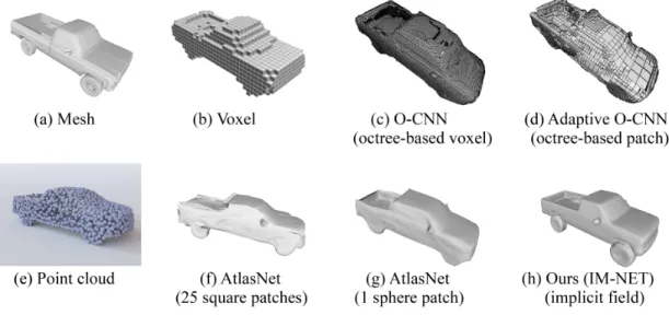
Figure 2.1 Visualizations of different shape representations. We choose to show trucks for those representations, but they are not necessarily the same truck. (a) Triangular mesh. (b) Voxel model; the image is from 3D-R2N2 [10]. (c) Voxel model generated by octree; the image is from Adaptive O-CNN [48]. (d) Patch-based model generated by octree; the image is from Adaptive O-CNN [48]. (e) Point cloud; the image is from [1]. (f) Deformable patches with 25 square patches as warping template. (g) Deformable patches with one closed sphere as warping template. (h) Implicit field generated by our model; the mesh is extracted by marching cubes. . . 5

(9)

Figure 3.1 illustration of point sampling process. (a) Obtaining the voxel models in different resolutions. (b) sampling points on each resolution. In (b) we do not show randomly sampled points in approach (1) and (2) for simplicity. We do not show approach (3) since all points in (3) are randomly sampled. . . 10

Figure 4.1 AE reconstruction samples during the training process. . . 14 Figure 4.2 AE interpolation results. . . 14 Figure 4.3 VAE interpolation results. The images in the box are the ones

show-ing the shape “A” crossshow-ing the gap. . . 15 Figure 4.4 WGAN results. We use two rows for each set of samples: the first

row is generated samples with random initialized latent vectors, the second row shows an interpolation sequence. . . 16

Figure 5.1 Visual results for 3D reconstruction. Each column presents one ex-ample from one category. IM-AE64 is sex-ampled on 643 resolution and IM-AE256 on 2563. All results are rendered using the same Marching Cubes setup. . . 18 Figure 5.2 3D shape interpolation results. 3DGAN, CNN-GAN, and IM-GAN

are sampled at 643resolution to show the smoothness of the surface is not just a matter of sampling resolution. Notice that the morphing sequence of IM-GAN not only consists of smooth part movements (legs, board), but also handles topology changes. . . 20 Figure 5.3 3D shape generation results. One generated shape from each category

is shown for each model; more results are available in the supplemen-tary material. Since the trained models of 3DGAN did not include plane category, we fill the blank with another car. The ball-pivoting method [7] was used for mesh reconstruction (c) from PC-GAN re-sults (b). . . 21 Figure 5.4 Visual results for 2D shape generation. The first part of each row

presents an interpolation between 9 and 6, except for DCGAN s-ince it failed to generate number 6 or 9. The second part of each row shows some generated samples. The sampled images are not bi-narized. More samples and binarized images can be found in the supplementary material. . . 22 Figure 5.5 Visual results for single-view 3D reconstruction. See caption of

(10)

Chapter 1

Introduction

Unlike images and video, 3D shapes are not confined to one standard representation. Up to date, deep neural networks for 3D shape analysis and synthesis have been developed for voxel grids [10, 49], octrees [19, 47, 48], multi-view images [42], point clouds [1, 36], and integrated surface patches [17]. Specific to generative modeling of 3D shapes, despite the many progresses made, the shapes produced by state-of-the-art methods still fall far short in terms of visual quality. This is reflected by a combination of issues including low-resolution outputs, overly smoothed or discontinuous surfaces, as well as a variety of topological noise and irregularities.

In this paper, we explore the use of implicit fields for learning deep models of shapes and introduce animplicit field decoder for shape generation, aimed at improving the visual quality of the generated models, as shown in Figure 1.1. An implicit field assigns a value to each point (x, y, z). A shape is represented by all points assigned to a specific value and is typically rendered via iso-surface extraction such as Marching Cubes. Our implicit field decoder, or simply implicit encoder, is trained to perform this assignment task, by means of abinary classifier, and it has a very simple architecture; see Figure 1.2. Specifically, it takes a point coordinate (x, y, z), along with a feature vector encoding a shape, and outputs a value which indicates whether the point is outside the shape or not. In a typical application setup, our decoder, which is coined IM-NET, would follow an encoder which outputs the shape feature vectors and then return an implicit field to define an output shape.

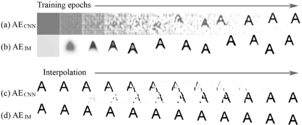
Several novel features of IM-NET impact the visual quality of the generated shapes. First, the decoder output can be sampled at any resolution and is not limited by the res-olution of the training shapes; see Figure 1.1. More importantly, we concatenate point coordinates with shape features, feeding both as input to our implicit decoder, which learns the inside/outside status of any point relative to a shape. In contrast, a classical convolution/deconvolution-based neural network (CNN) operating on voxelized shapes is typically trained to predict voxels relative to the extent of the bounding volume of a shape. Such a network learns voxel distributions over the volume, while IM-NET learns shape boundaries; this is well exemplified in Figure 1.3 (top). Experiments show that shapes

(11)

gen-Figure 1.1: 3D shapes generated by IM-GAN, ourimplicit field generative adversarial net-work, which was trained on 643 _{voxelized shapes for chair category and 128}3 _voxelized

shapes for car and plane category. The output shapes are sampled at 5123 resolution and rendered after Marching Cubes.

Figure 1.2: Network structure of our implicit decoder, IM-NET. The network takes as input a feature vector extracted by a shape encoder, as well as a 3D or 2D point coordinate, and it returns a value indicating the inside/outside status of the point relative to the shape. The encoder can be a CNN or use PointNET [36], depending on the application.

erated by our network possess higher surface quality than results from previous methods, as shown in Figure 1.1 and results in Chapter 5.

In addition, shape evolution is a direct result of changing the assignments of point coor-dinates to their inside/outside status and such assignments are precisely what our network, IM-NET, learns. In contrast, convolution kernels compute voxels as weighted averages, where the kernel windows are not “shapaware”. Thus a CNN-based decoder typically e-volves shape geometries by means of intensity variations; see Figure 1.3 (bottom). As a result, our network produces cleaner interpolation results than previous works, even when there are topological changes; see Figure 5.2.

We embed IM-NET into several contemporary analysis and synthesis frameworks, in-cluding autoencoders (AEs), variational autoencoders (VAEs), and generative adversarial networks (GANs), by replacing the decoders employed by current approaches with ours,

(12)

Figure 1.3: CNN-based decoder vs. our implicit decoder. We trained two autoencoders with CNN decoder (AECNN) and our implicit decoder (AEIM), respectively, on a synthesized

dataset of letter A’s on white background. The two models have the same CNN encoder. (a) and (b) show the sampled images during AE training. (c) and (d) show interpolation sequences produced by the two trained AEs. See more comparisons in Chapter 4.

leading to IM-AEs and IM-GANs. This allows assessing the capabilities of our novel de-coder for tasks such as shape representation learning, 2D or 3D shape generation, shape interpolation, as well as single-view 3D shape reconstruction. Extensive experiments and comparative studies, both quantitative and qualitative, demonstrate the superiority of our network over previous works, particularly in terms of visual quality.

(13)

Chapter 2

Related work

2.1 Shape representations

There have been a variety of 3D shape representations for deep learning of shapes, such as voxel grids [10, 15, 31, 49, 50], octrees [19, 38, 44, 47, 48], multi-view images [32, 42], point clouds [1, 13, 14, 36, 35, 51, 52], geometry images [40, 41], deformable mesh/patches [17, 41, 46, 51], and part-based structural graphs [29, 53]. To the best of our knowledge, our work is the first to introduce a deep network for learning implicit fields for generative shape modeling. See Figure 2.1 for some visualizations of those different representations.

For generative models, the output shape representation is crucial, for it determines the visual quality of the output shapes. Triangular mesh is the ideal and mostly used representation in the Graphics community. But currently, meshes are not compatible with neural networks, since neural networks require the input and output to be some fixed format, therefore they cannot handle those irregular meshes with a varying number of vertices and complex connections.

Voxel representation is also very popular, since its counterpart, pixel representation, is the dominant representation for images in almost all image related tasks. However, it is not an easy task to adapt pixel-based methods for image processing to voxel-based methods for shape processing, because the extra dimension in the 3D space brings higher complexity in both storage and computation. For instance, a 256×256 image only takes 65,536 pixels to store, which is roughly 262 KB if we store pixels as float numbers; but a 256×256×256 voxel model needs 16,777,216 voxels to store, which is roughly 67 MB if we store voxels as float numbers. Such costs are prohibitive for directly using high-resolution voxel models, therefore some other methods utilize octrees to reduce the storage and computational costs. But due to the inherent properties of CNN models, the generated shapes usually do not possess smooth surfaces, which makes them less visually pleasing. We will discuss the differences between our model and CNN model in Chapter 4.

Point cloud is another popular representation. Although how to order the points to fit them into the network input format may seem to be a problem, it can be solved by various

(14)

Figure 2.1: Visualizations of different shape representations. We choose to show trucks for those representations, but they are not necessarily the same truck. (a) Triangular mesh. (b) Voxel model; the image is from 3D-R2N2 [10]. (c) Voxel model generated by octree; the image is from Adaptive O-CNN [48]. (d) Patch-based model generated by octree; the image is from Adaptive O-CNN [48]. (e) Point cloud; the image is from [1]. (f) Deformable patches with 25 square patches as warping template. (g) Deformable patches with one closed sphere as warping template. (h) Implicit field generated by our model; the mesh is extracted by marching cubes.

methods [4, 30, 36]. But most of them focus on the encoding phase, which needs invariance to point order. But for point-cloud generative models, most of them simply use several fully connected layers to generate an array of points, and such decoders are anything but point-order invariance. In addition, while it is natural for CNN decoders to make some part of the shape “disappearing” or “emerging” in an interpolation sequence, point-cloud based models typically cannot, since they always output a fixed number of points. When interpolating, the points of the “emerging” parts will be taken from existing parts, and the points of the “disappearing” parts will be merged into other remaining parts. So far there is no solution to this problem. Another drawback of point clouds is that they do not look good. Typically people generate 1,024, 2,048 or 4,096 points in their networks, which are not enough to reconstruct a high-resolution mesh.

Deformable mesh/patches are recently-proposed representations that can partially fix the reconstruction issues of point clouds, since they warp one or several already given template patches to the target shape. Therefore, the network output will already be a mesh. But such methods rely too much on the templates. For instance, in AtlasNet [17], the authors use two kinds of templates: 25 square patches, or one sphere. When using 25 square patches as template, the output shape will be made of 25 patches, so the slits, overlaps, and

(15)

foldovers are visible and affect the eventual visual quality of the output mesh. When using one sphere as template, the output shape will have a pre-assigned topology of a sphere, which limits the representation ability of the output mesh. And similar to point clouds, deformable mesh/patches cannot deal with part “disappearing” or “emerging” issues, since the vertices and connectivities of the final mesh are pre-assigned.

Our implicit field representation is different from all the representations above. The decoder of our network approximates an implicit field of the target shape, and the final mesh is extracted via marching cubes. In training, the decoder needs not to generate all voxels in a voxel model, but a selected few near the shape surfaces, which solves the storage and computational complexity issue. The representation is continuous in the output 2D or 3D space comparing to the CNN models, which makes the output shapes smoother and supports better shape interpolations. There are no pre-assigned templates, which allows our output shape to have varying topologies and better approximate a given shape. The network does not forbid part “disappearing” or “emerging”; also, the point-coordinate-as-input decoder allows shape/part movement by adjusting the point-coordinate-as-input point coordinates in the hidden layers. Our implicit field representation combines several good properties of the above representations and solves most issues.

2.2 Generative models of 3D shapes

With remarkable progress made on generative modeling of images using VAEs [26], GAN-s [3, 16, 37], autoregreGAN-sGAN-sive networkGAN-s [45], and flow-baGAN-sed modelGAN-s [25], there have been considerably fewer works on generative models of 3D shapes. Girdhar et al. [15] learned an embedding space of 3D voxel shapes for 3D shape inference from images and shape genera-tion. Wu et al. [49] extended GANs from images to voxels and their 3DGAN was trained to generate 3D voxel shapes from latent vectors. Achlioptas et al. [1] proposed a latent-GAN workflow that first trains an autoencoder with a compact bottleneck layer to learn a latent representation of point clouds, then trains a plain GAN on the latent code. Common issues with these methods include limited model resolution, uneven and noisy shape surfaces, and inability to produce smooth shape interpolation.

Recently, Li et al. [29] introduced a part-based autoencoder for 3D shape structures, i.e., a hierarchical organization of part bounding boxes. The autoencoder is tuned with an adversarial loss to become generative. Then a separate network is trained to fill in part geometries within the confines of the part bounding boxes. Their method can produce cleaner 3D shapes and interpolation results, mainly owing to the decoupling of structure and geometry generation. However, their network has to be trained by segmented shapes with structural hierarchies. In contrast, our implicit encoder is trained on unstructured voxel shapes.

(16)

2.3 Image superresolution

The output of our decoder IM-NET can be sampled at resolutions higher than that of the training shapes, however, it is not designed for the purpose of(voxel) super-resolution. There have been works on single image super-resolution using deep networks, e.g., [12, 27], which are trained with low- and high-resolution image pairs. Progressive training [24] is another technique to improve image quality, and we adopt it in our work to reduce training times.

2.4 Single-view reconstructions

Reconstructing the object shape from a single image is both challenging and ill-posed, for one shape can have infinite number of views and one view can have multiple corresponding shapes due to occlusion. With the release of large-scale 3D shape datasets like ShapeNet [8], data-driven methods like deep neural networks have achieved great progress in recent years. Most learning-based methods for single-view 3D reconstruction encode input images with deep convolutional networks, then use an appropriate decoder to reconstruct 3D shapes depending on the shape representations. The most commonly used representations are vox-els [10, 15, 50] and point clouds [13, 14]. Voxvox-els are natural extensions of image pixvox-els, which allow migrating state-of-the-art techniques from image processing to shape process-ing. However, voxel representations are usually constrained by GPU memory size, resulting in low-resolution results. Octree representations attempt to fix the memory issues by pre-dicting surfaces in a coarse-to-fine manner [19, 48].

The recent work by Huang et al. [23] also trains a network to perform binary classifica-tion, like IM-NET. However, the key distinction is that our network assigns inside/outside based on spatial point coordinates. Hence, it learns shape boundaries and effectively, an implicit function that isLipschitz continuous over point coordinates, i.e., it maps close-by points to similar output values. Moreover, IM-NET can input an arbitrary 3D point and learn a continuous implicit field without discretization. In contrast, their network operates on convolutional features computed over discretized images and learns the inside/outside assignment based on multi-scale image features at a pointx.

Point clouds can be lightweight on the decoder side by producing few thousand points. However, these points do not provide any surface or topological information and pose a reconstruction challenge. In Deep Marching Cubes, Liao et al. [31] proposed a differentiable formulation of marching cubes to train an end-to-end 3D CNN model for mesh reconstruc-tion from point clouds. However, the resulting mesh still shares common issues with other CNN-based networks, e.g., low resolution (323) and topological noise.

Some other works [17, 41] deform a surface template (e.g., square patches or a sphere) onto a target shape. But many shapes cannot be well-represented by a single patch, while outputs from multi-patch integrations often contain visual artifacts due to gaps, foldovers, and overlaps.

(17)

In contrast to the above methods, some methods exploit input images in pixel level. Some part based approaches [22, 43] retrieve shape components from existing shapes then assemble and deform them to fit the observed image. In Pixel2Mesh, Wang et al. [46] used a graph-based CNN [39] to progressively deform an ellipsoid template to fit an image. It assigns different perceptual features extracted from the input image for different vertices according to their projected positions on the image. The end-to-end network directly generates meshes but the results tend to be overly smoothed, capturing only low-frequency features while restricted to sphere topology.

(18)

Chapter 3

Implicit decoder

3.1 Theoretical Motivation

An implicit field is defined by a continuous function over 2D/3D space. Then a mesh sur-face can be reconstructed by finding the zero-isosursur-face of the field with methods such as Marching Cubes [33]. In our work, we consider using neural networks to describe a shape in such an implicit way. For a closed shape, we define the inside/outside fieldF of the shape by taking the sign of its signed distance field:

F(p) = (

0 if point pis outside the shape,

1 otherwise. (3.1)

Assume the in-out field is restricted in a unit 3D space, we attempt to find a parameter-ization fθ(p) with parameters θ that maps a point p ∈ [0,1]3 to F(p). This is essentially

a binary classification problem, which has been studied very well. Multi-layer perceptrons (MLPs) with rectified linear unit (ReLU) nonlinearities are ideal candidates for such tasks. With sufficient hidden units, MLP family is able to approximate the field F within any precision. This is a direct consequence of the universal approximation theorem [21]. Notice that using MLPs also gives us a representation which is continuous across space, so that the mesh can be recovered by taking thek-isosurface of the approximated field, where kis an appropriate threshold.

3.2 Data preparation

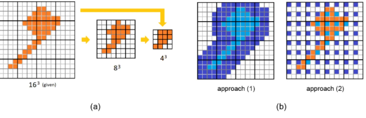
The training of such implicit model needs point-value pairs. It is natural to first voxelize or rasterize the shape for the sake of convenience and uniform sampling. For 3D shapes, we use the same technique as in Hierarchical Surface Prediction (HSP) [19] to get the voxel models in different resolutions. Assume the 2563 voxel models are given, at each resolution (163, 323, 643, 1283), we label a voxel occupied if this voxel contains at least one occupied voxel in the 2563 model.

(19)

Figure 3.1: illustration of point sampling process. (a) Obtaining the voxel models in different resolutions. (b) sampling points on each resolution. In (b) we do not show randomly sampled points in approach (1) and (2) for simplicity. We do not show approach (3) since all points in (3) are randomly sampled.

Then we sample points on each resolution in order to train the model progressively. A naive sampling would take the center of each voxel and produce n3 _{points. A more}

efficient approach when dealing with shapes is to sample more points near shape surfaces and neglect most points far away, leading to roughlyO(n2) points. Specifically, we sample each resolution with the following number of point-value pairs: for 163 _{voxel grid resolution,}

we sample all the points in the grid (4,096 points); for 323, we sample 8,192 points; for 643, we sample 32,768 points; for 1283, we sample 131,072 points. We use one of the three following sampling approaches, see an illustration in Figure 3.1

(1) Sample points which are within 3 voxels (in all x, y, z directions) from shape bound-aries. If the number of sampled points does not exceed the limit, randomly sample more points up to the limit.

(2) If (1) fails, sample points every two voxels in all x, y, z directions. If the number of sampled points does not exceed the limit, randomly sample more points up to the limit.

(3) If (2) fails, randomly sample points up to the limit.

To compensate for the density change, we assign a weight wp to each sampled point p, representing the inverse of the sampling density near p. The implementation of such a sampling method is flexible and varies according to resolution and shape category. In practice we assigned weights of all sampled points to 1, because we want the model to pay more attention to the surface and allow small error in the void area.

Most 2D shapes are already rasterized into images. For simplicity, we apply the naive sampling approach for images with an appropriate threshold to determine whether a pixel belongs to the shape.

(20)

3.3 Network structure

Our model is illustrated in Figure 1.2. The skip connections (copy and concatenate) in the model can make the learning progress faster in the experiments. They can be removed when the feature vector is long, so as to prevent the model from becoming too large. The loss function is a weighted mean squared error between ground truth labels and predicted labels for each point. LetS be a set of points sampled from the target shape, we have:

L(θ) = P p∈S|fθ(p)− F(p)|2·wp P p∈Swp (3.2)

3.4 Shape generation and other applications

Our implicit field decoder, IM-NET, can be embedded into different shape analysis and synthesis frameworks to support various applications. In this paper, we demonstrate shape autoencoding, 2D and 3D shape generation, and single-view 3D reconstruction. Due to page limit, the models are briefly introduced here. Detailed structures and hyperparameters can be found in the supplementary material.

For auto-encoding 3D shapes, we used a 3D CNN as encoder to extract 128-dimensional features from 643 voxel models. We adopt progressive training techniques, to first train our model on 163 _{resolution data, then increase the resolution gradually. Notice that the}

structure of the model does not change when switching between training data at different resolutions, thus higher-resolution models can be trained with pre-trained weights on low-resolution data. In the experiments, progressive training can stabilize training process and significantly reduce training time.

For 3D shape generation, we employed latent-GANs [1, 2] on feature vectors learned by a 3D autoencoder. We did not apply traditional GANs trained on voxel grids since the training set is considerably smaller compared to the size of the output. Therefore, the pre-trained AE would serve as a means for dimensionality reduction, and the latent-GAN was trained on high-level features of the original shapes. We used two hidden fully-connected layers for both the generator and the discriminator, and the Wasserstein GAN loss with gradient penalty [3, 18]. In generative models for 2D shapes, we used the same structure as in the 3D case, except the encoder was 2D CNN and the decoder took a 2D point as input. We did not apply progressive training for 2D shapes since it is unnecessary when the images are small.

For single-view 3D reconstruction (SVR), we used the ResNET [20] encoder to obtain 128-D features from 1282 images. We followed the idea from AtlasNET [17] to first train an autoencoder, then fix the parameters of the implicit decoder when training SVR. In our experiments, we adopted a more radical approach by only training the ResNET encoder to minimize the mean squared loss between the predicted feature vectors and the ground truth.

(21)

This performed better than training the image-to-shape translator directly, since one shape can have many different views, leading to ambiguity. Pre-trained decoders provide strong priors that can not only reduce such ambiguity, but also shorten training time, since the decoder was trained on unambiguous data in the autoencoder phase and encoder training was independently from the decoder in SVR phase.

We reconstructed the 3D meshes by Marching Cubes, and 2D images by sampling a grid of points then optionally applying thresholding to obtain binarized shapes.

(22)

Chapter 4

Comparison with CNN decoder

In this chapter, we provide several toy experiments to compare the different features learned by CNN-based models and implicit-decoder-based models. We use subscripts X_CNNand X_IM to distinguish models with different decoders throughout this chapter.

4.1 Training data

The training dataset is synthesized by putting binarized letter “A”s on white background. The image of “A” is 29×27 (height×width), and the image size for the dataset is 64×64, therefore we have 35×37 possible positions to put the whole A in the image, and that makes our dataset contain 35×37 = 1295 images.

We have two versions of the dataset, A and A_blur. A_blur contains blurred “A”s which are Gaussian blurred with sigma = 1.

Besides, we have incomplete versions of the above datasets. We removed the middle four rows of possible positions of A, resulting in 31×37 possible positions. We call the incomplete versionsA_gapand A_gap_blurrespectively. Such dataset can test the model’s ability to generate unseen shapes to fill the gap.

4.2 Autoencoder (AE)

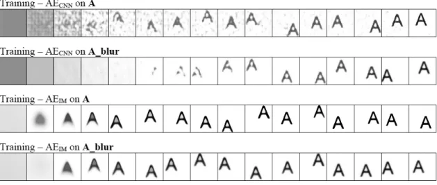
We trained AEs with CNN decoder and implicit decoder onA andA_blur. In Figure 4.1 we show AE reconstruction samples during the training process.

One can get a feel about the features learned by different decoders. AECNNis predicting

the possibility for each specific pixel to be on or off, while AE_IM is learning the field of the shape. In Figure 4.2 we show AE interpolation results, to show the movement is learned by AEIM while AECNN is simply memorizing each specific shape.

(23)

Figure 4.1: AE reconstruction samples during the training process.

Figure 4.2: AE interpolation results.

4.3 Variational Autoencoder (VAE)

We trained VAEs on A_gap and A_gap_blur. VAE constraints the latent space to be compact, therefore the interpolation with VAE is much better for CNN based models. But can those models generate unseen new shapes to fill the gap? In Figure 4.3 we show VAE interpolation results when crossing the gap. Notice the fractured shapes when VAECNN is

crossing the gap. It shows that VAE with CNN decoder is not able to generate new shapes by simply moving the entire shape around, due to the inherent movement-discontinuity of CNN in the output image space.

(24)

Figure 4.3: VAE interpolation results. The images in the box are the ones showing the shape “A” crossing the gap.

4.4 Wasserstein GAN (WGAN)

We did not train WGANs on A_gap and A_gap_blur, since the discriminator may consider shapes crossing the gap as negative samples and prohibit the generator from gen-erating such samples. We trained WGANs on Aand A_blur, to show shape movement is not continuous in the output space of CNN decoders. The result in shown in Figure 4.4. We use two rows for each set of samples: the first row is generated samples with random initialized latent vectors, the second row shows an interpolation sequence.

The perception of continuity for CNN decoders is the lightness change in each pixel, therefore dataset A is far from continuous in WGAN_CNN’ eyes. A direct consequence is that WGANCNN cannot be trained well on datasetA. But if we blur the images to provide

such lightness changes and make the dataset continuous in WGAN_CNN’s perception, it will get good results, see the results from WGANCNN trained on A_blur.

As for the implicit decoder, both lightness changes and shape movements are continuous, therefore it can be trained well on bothA and A_blur.

(25)

Figure 4.4: WGAN results. We use two rows for each set of samples: the first row is gener-ated samples with random initialized latent vectors, the second row shows an interpolation sequence.

(26)

Chapter 5

Experiments and evaluation

In this chapter, we show qualitative and quantitative results on various tasks using our implicit decoder, IM-NET, and compare them with state-of-the-art approaches. We used the dataset provided by [19], which contains 2563-voxelized and flood-filled 3D models from ShapeNet Core dataset (v1) [8], and the corresponding rendered views. To compare with other methods that output point clouds, we first used Marching Cubes to obtain meshes from the 2563-voxelized models, then used Poisson-disk Sampling [11] to obtain 10000 points. This gave us point clouds with only points on the surfaces of the meshes. We evaluated our method, and others, on five representative categories: plane, car, chair, rifle, and table. These categories contain 4,045, 7,497, 6,778, 2,373, and 8,509 3D shapes, respectively.

5.1 Quality metrics

In our experiments, both qualitative (via visual examination) and quantitative evaluations are provided. Specific to shapes, most evaluation metrics for encoding and reconstruction are based on point-wise distances, e.g., chamfer distance (CD), or global alignment, e.g., mean squared error (MSE) and intersection over union (IoU) on voxels. However, these may not be the best visual similarity or quality metrics. For example, slightly adjusting the angles between the legs of a chair and its seat may be barely perceptible, compared to removing one shape part, yet the latter could lead to a lower CD or IoU. Past works, e.g., [34], have shown that low-frequency displacements (e.g., bending a leg) in shapes are less noticeable than high-frequency errors over local surface characteristics such as normals and curvatures. Metrics such as MSE, CD, and IoU do not account for visual quality of the object surfaces.

A less frequently used visual similarity metric in the computer vision community, the light field descriptor (LFD) [9], has been widely adopted in computer graphics. Inspired by human vision system, LFD considers a set of rendered views of a 3D shape from various camera angles. Each projected image is then encoded using Zernike moments and Fourier descriptors for similarity comparisons.

(27)

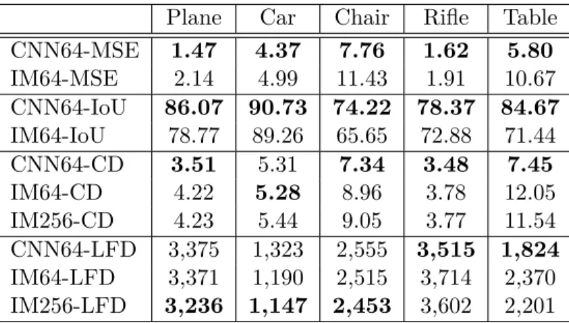
Plane Car Chair Rifle Table CNN64-MSE 1.47 4.37 7.76 1.62 5.80 IM64-MSE 2.14 4.99 11.43 1.91 10.67 CNN64-IoU 86.07 90.73 74.22 78.37 84.67 IM64-IoU 78.77 89.26 65.65 72.88 71.44 CNN64-CD 3.51 5.31 7.34 3.48 7.45 IM64-CD 4.22 5.28 8.96 3.78 12.05 IM256-CD 4.23 5.44 9.05 3.77 11.54 CNN64-LFD 3,375 1,323 2,555 3,515 1,824 IM64-LFD 3,371 1,190 2,515 3,714 2,370 IM256-LFD 3,236 1,147 2,453 3,602 2,201

Table 5.1: 3D reconstruction errors. CNN and IM represent CNN-AE and IM-AE, respec-tively, with 64 and 256 indicating sampling resolutions. The mean is taken over the first 100 shapes in each tested category. MSE is multiplied by 103, IoU by 102, and CD by 104. LFD is rounded to integers. Better-performing numbers are shown in boldface.

Figure 5.1: Visual results for 3D reconstruction. Each column presents one example from one category. IM-AE64 is sampled on 643 resolution and IM-AE256 on 2563. All results are rendered using the same Marching Cubes setup.

5.2 Auto-encoding 3D shapes

We first compare IM-NET with CNN decoders. For each category, we sorted the shapes by name and used the first 80% as training set and the rest for testing. We trained one model with our implicit decoder (IM-AE) and another with 3D CNN decoder (CNN-AE) on each category. The 3D CNN decoder is symmetric to the 3D CNN encoder (details can be found in the supplementary material). Both models had the same encoder structure and were

(28)

trained on 643 resolution for the same number of epochs between 200 and 400, depending on the size of the dataset.

Table 5.1 evaluates reconstruction results using several common evaluation metrics: MSE, IoU, symmetric Chamfer distance (CD), and LFD. MSE and IoU were computed against the ground truth 643 voxel models. For CD and LFD, we obtained meshes from the output voxel models by Marching Cubes with threshold 0.5. We sampled 2,048 points from the vertices for each output mesh and compare against ground truth point clouds to compute CD. Note that CNN-AE has fixed output size (643), yet our implicit model can be up-sampled to arbitrarily high resolution by adjusting the sampling grid size. In Table 5.1, IM256 is the same IM-AE model but sampled at 2563.

Although CNN-AE beats IM-AE in nearly all five categories in terms of MSE, IOU, and CD, visual examination clearly reveals that IM-AE produces better results, as shown in Figure 5.1; more such results are available in the supplementary material. This validates that LFD is a better visual similarity metric for 3D shapes. On one hand, the movement of some parts, for example, table boards, may cause significant MSE, IOU and CD changes, but bring little visual changes; on the other hand, legs are usually thin, so that missing one leg may cause minor MSE, IOU and CD changes, but can bring significant visual changes. As remarked above, MSE, IOU and CD do not capture well surface quality: a smooth but not exactly aligned surface might have poorer evaluation results than an aligned jagged surface. The situation is better when using LFD. However, since LFD only renders the silhouette of the shape without lighting, it can only capture surface condition on the edge of the silhouette. We expect better evaluation metrics to be proposed in the future, and for the following experiments, we use LFD as our primary evaluation metric.

Note that in the table example in Figure 5.1, a 643 resolution represents an under-sampling, while going up to 2563 reveals more details. This indicates that our generative model is able to generate a table board thinner than the resolution of the training data, which shows that the model learned the implicit field from the whole shape in the space rather than merely learning voxel distributions.

5.3 3D shape generation and interpolation

Next, we assess and evaluate improvements made by our implicit decoder for generative modeling of 3D shapes. We trained latent-GANs on both CNN-AE and IM-AE to obtain CNN-GAN and IM-GAN. We also compared our results with two state-of-the-art methods, 3DGAN [49] and the generative model for point clouds in [1] (PC-GAN). For 3DGAN, we used the trained models made available online by the authors. PC-GAN was trained using latent WGAN [1]. The autoencoder of PC-GAN was trained on our aforementioned point cloud data for 400 epochs for each category. PC-GAN, CNN-GAN, and IM-GAN were

(29)

Figure 5.2: 3D shape interpolation results. 3DGAN, CNN-GAN, and IM-GAN are sampled at 643 resolution to show the smoothness of the surface is not just a matter of sampling resolution. Notice that the morphing sequence of IM-GAN not only consists of smooth part movements (legs, board), but also handles topology changes.

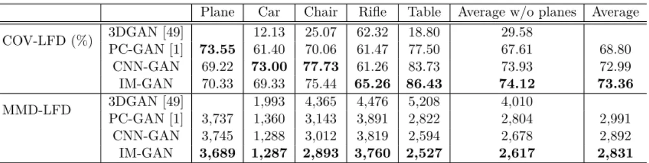
Plane Car Chair Rifle Table Average w/o planes Average COV-LFD (%) 3DGAN [49] 12.13 25.07 62.32 18.80 29.58 PC-GAN [1] 73.55 61.40 70.06 61.47 77.50 67.61 68.80 CNN-GAN 69.22 73.00 77.73 61.26 83.73 73.93 72.99 IM-GAN 70.33 69.33 75.44 65.26 86.43 74.12 73.36 MMD-LFD 3DGAN [49] 1,993 4,365 4,476 5,208 4,010 PC-GAN [1] 3,737 1,360 3,143 3,891 2,822 2,804 2,991 CNN-GAN 3,745 1,288 3,012 3,819 2,594 2,678 2,892 IM-GAN 3,689 1,287 2,893 3,760 2,527 2,617 2,831

Table 5.2: Quantitative evaluation of 3D shape generation. LFD is rounded to integers. See texts for explanation of the metrics.

trained on the training split of the dataset for 10,000 epochs. 3DGAN was not trained using train/test split [49].

To compare the generative schemes, we adopted the evaluation metrics from [1], but replaced CD or EMD by LFD. Suppose that we have a testing setGand a sample setA, for each shape inA, we find its closest neighbor inGusing LFD, sayg, and markgas “matched”. In the end, we calculate the percentage of G marked as “matched” to obtain the coverage score (COV-LFD) that roughly represents the diversity of the generated shapes. However, a random set may have a high coverage, since matched shapes need not be close. Therefore, we match every shape in G to the one in A with the minimum distance and compute the

(30)

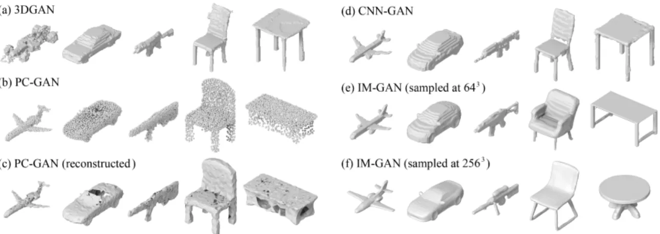
Figure 5.3: 3D shape generation results. One generated shape from each category is shown for each model; more results are available in the supplementary material. Since the trained models of 3DGAN did not include plane category, we fill the blank with another car. The ball-pivoting method [7] was used for mesh reconstruction (c) from PC-GAN results (b).

mean distances in the matching as Minimum Matching Distance (MMD-LFD). Ideally, a good generative model would have higher COV-LFD and lower MMD-LFD values.

We first sampled shapes using the subject generative model to obtain A, where the number of sampled shapes is five times the number of shapes in the testing split (G) of that category. For PC-GAN, we employed the ball-pivoting method [7] to reconstruct the shape surface, while for all the other generative models, we used Marching Cubes. IM-GAN was sampled at 643 in quantitative evaluation.

Quantitative and qualitative evaluations are shown in Table 5.2 and Figure 5.3, respec-tively. Overall, IM-GAN performs better on both COV-LFD and MMD-LFD. More impor-tantly, IM-GAN generates shapes with better visual quality compared to other methods, in particular, with smoother and more coherent surfaces. 3DGAN appears to suffer from mode collapse on several categories, leading to lower coverage. Point clouds generated by PC-GAN are recognizable but lack detailed features; high-quality reconstruction from only 2048 generated points would be challenging. In addition, as shown in Figure 5.2, IM-GAN exhibits superior capability in 3D shape interpolation. As usual for the latent generative models, the interpolation is carried out by a linear interpolation between two latent codes; in-between 3D shapes are then generated from the intermediate codes.

We trained the IM-GAN further with 1283 resolution data on category plane, car and rifle. Figure 1.1 shows some results sampled at 5123. We also include, in the supplementary material, videos showing interpolation results of IM-GAN sampled at 2563, and comparisons between interpolations in IM-AE and IM-GAN latent spaces.

(31)

DCGAN [37] CNN-GAN IM-GAN VAE [26] VAEIM WGAN [18] WGANIM Oracle COV-CD (%) 3.9 82.7 75.2 72.1 74.9 86.5 84.7 88.4 MMD-CD 0.846 0.155 0.151 0.145 0.14 0.158 0.149 0.137 PWE (nat) -282.83 -8.07 -6.16 17.39 30.6 -24.54 -4.17 18.99 PWE-nb (nat) -230.47 130.93 128.38 304.57 318.07 97.32 93.1 241.19 IS [28] 3.26 8.79 9.36 9.09 9.42 8.9 9.22 9.8 IS-nb 3.26 8.8 9.39 7.58 8.28 8.95 9.22 9.88

Table 5.3: Quantitative evaluation for 2D shape generation. Oracle is the results obtained by using the training set as the sample set. The metrics without suffix “-nb” are evaluated using binarized images. PWE and IS are the higher the better. The better results in each subgroup (latent-GAN, VAE, WGAN) are bolded, and the best results over all models are underlined.

Figure 5.4: Visual results for 2D shape generation. The first part of each row presents an interpolation between 9 and 6, except for DCGAN since it failed to generate number 6 or 9. The second part of each row shows some generated samples. The sampled images are not binarized. More samples and binarized images can be found in the supplementary material.

5.4 2D shape generation and interpolation

To evaluate IM-GAN for 2D shape generation, we conducted our experiments on the MNIST dataset since hand-written digits are naturally 2D shapes. We compared our results against DCGAN [37], VAE [26], and WGAN with gradient penalty [3, 18]. We also included the 2D version of CNN-GAN. In addition, we substituted the CNN decoders of VAE and WGAN with our implicit decoders, to obtain VAEIM and WGANIM. We trained all models on

5,000 binarized images from the training split of MNIST dataset for 1,000 epochs. The training set contains a smaller-than-usual amount of images, so that we can better observe the different features learned by CNN models and implicit models. The autoencoders of IM-GAN and CNN-GAN were pre-trained for 200 epochs. We replace LFD with chamfer distance in 2D images to obtain COV-CD and MMD-CD for evaluation. We also report the inception score for MNIST (IS) [28] and the log-likelihood produced by Parzen-window estimate (PWE) [5, 6, 16]. For COV-CD and MMD-CD, we sampled 5,000 images from the subject models and compared against 1,000 ground truth images from the testing split. For IS and PWE, we sampled 10,000 images and used the entire testing split.

(32)

Plane Car Chair Rifle Table HSP 6,307 2,009 4,255 6,360 3,765 AtlasNet25 4,877 1,667 3,244 6,507 2,725

AtlasNetO 5,208 1,751 4,124 6,117 3,909 IM-SVR 4,743 1,658 3,321 5,067 2,918

Table 5.4: Quantitative evaluation for SVR using LFD. The means are taken over the first 100 shapes in the testing set for each category and rounded to integers. AtlasNet25 is AtlasNet with 25 patches (28,900 mesh vertices in total) and AtlasNetO (7,446 vertices) is with one sphere. IM-SVR and HSP were both reconstructed at 2563 resolution.

Plane Car Chair Rifle Table HSP 16.33 12.27 28.96 15.60 27.41 AtlasNet25 8.10 8.10 18.47 9.40 14.20

AtlasNetO 11.37 8.25 25.35 10.67 21.67 IM-SVR 9.74 9.68 22.09 10.57 18.97

Table 5.5: Quantitative evaluation for SVR using CD. The means are taken over the first 100 shapes in the testing set for each category. CD is multiplied by 104.

Quantitative and qualitative evaluations are shown in Table 5.3 and Figure 5.4, re-spectively. Models equipped with our implicit decoders generally perform better. Due to inadequate training samples, DCGAN suffers from mode collapse, suggesting that the W-GAN loss is preferred to extract true features with smaller training sets. VAEs have better performance over GANs when the output images are binarized, since VAEs tend to produce blurry results. For interpolation, CNN based methods tend to make old parts disappear and then new parts appear. This phenomenon is especially apparent in CNN-GAN and VAE. The implicit model usually warps the shape, but can also carry the “disappear and appear” trick. In visual comparison, IM-GAN and WGANIM output cleaner and more recognizable

“in-between” digits. One can find missing or redundant parts in the samples produced by CNN based methods, which are vestiges of the “disappear and appear” phenomenon.

5.5 Single-view 3D reconstruction (SVR)

We compare our approach with two state-of-the-art SVR methods, HSP [19], an octree-based method that uses 3D CNN decoders to generate 2563 voxels, and AtlasNet [17], which warps surface patches onto target shapes. For AtlasNet, we tested two setups for the initial surfaces, 25 patches or a sphere, and denote them by AtlasNet25 and AtlasNetO, respectively. For all methods, we trained individual models for each category, and used grayscale images as inputs.

(33)

Figure 5.5: Visual results for single-view 3D reconstruction. See caption of Table 5.4 for output model settings.

We used the train/test split in [19] to utilize the pre-trained models of HSP, since HSP requires quite a long time to converge. For HSP, we used the trained models made available

(34)

online by the authors, and continued training for at most 2 days for each category and used the ones with the lowest testing loss. For AtlasNet, we trained the autoencoder part for 400 epochs and SVR part for 400 epochs and used the ones with the lowest testing loss. For our method, we trained IM-AE for 200-400 epochs on 643 resolution, and IM-SVR for 1,000-2,000 epochs. The number of epochs depends on the size of the dataset. We did not train AtlasNet with such number of epochs since its testing loss had stopped dropping. Since IM-SVR was trained to map an image into a latent code, we did not have a good evaluation metric for testing errors. Therefore, we tested the last five saved checkpoints and report the best results.

Quantitative and qualitative evaluations are shown in Table 5.4 and Figure 5.5, re-spectively. IM-SVR outputs were sampled at 2563 resolution, same as HSP. Output mesh settings for AtlasNet are from the authors’ code. Though IM-SVR seems to have similar quantitative results with AtlasNet25, please keep in mind that LFD only captures the sil-houette of the shape. AtlasNet25 represents shapes well yet clear artifacts can be observed since the shapes are made of patches and there is no measure to prevent slits, foldovers or overlapped surfaces. AtlasNetO can generate cleaner shapes than AtlasNet25, but the topology is pre-assigned to be equivalent to a sphere, thus AtlasNetO can hardly reconstruct shapes with holes. HSP can produce smooth surfaces but failed to recover most details. We provide the evaluation results by chamfer distance in Table 5.5 to further verify that CD may not be an ideal evaluation metric for visual quality.

(35)

Chapter 6

Limitation and future work

A key merit of our implicit encoder is the inclusion of point coordinates as part of the input feature, but this comes as the cost of longer training time, since the decoder needs to be applied on each point in the training set. In practice, CNN-AE is typically 30 times faster than IM-AE on 643 data without progressive training. Even with progressive training, IM-AE training took about a day or two and CNN-IM-AE is still 15 times faster. When retrieving generated shapes, CNN only needs one shot to obtain the voxel model, while our method needs to pass every point in the voxel grid to the network to obtain its value, therefore the time required to generate a sample depends on the sampling resolution. While AtlasNet also employed MLP as decoder, AtlasNet25 is 5 times faster than ours in training, since AtlasNet only needs to generate points on the surface of a shape yet ours need to generate points in the whole field.

Our implicit decoder does lead to cleaner surface boundaries, allowing both part move-ment and topology changes during interpolation. However, we do not yet know how to regulate such topological evolutions to ensure a meaningful morph between highly dissimi-lar shapes, e.g., those from different categories. We reiterate that currently, our network is only trained per shape category; we leave multi-category generalization for future work. At last, while our method is able to generate shapes with greater visual quality than existing alternatives, it does appear to introduce more low-frequency errors (e.g., global thinning/thickening).

Compared to IoU, MSE, and CD, LFD may be a better visual similarity metric, but still far from ideal. An evaluation metric that fits human perception could be of great interest to the graphics community, and deserves more attention.

In future work, we also plan to generalize IM-NET. First, using MLPs to decode may be too simple and inefficient; it is possible to improve the decoder structure to make the model size smaller for faster inference. Second, besides inside/outside signs, it is possible to train our decoder to output other attributes, e.g., color, texture, surface normal, signed distance, or deformation fields, for new applications. Third, IM-NET has shown signs of un-derstanding shape parts, suggesting its potential utility for learning part segmentation and

(36)

correspondence. Finally, the implicit field representation provides an easy way to combine synthesized parts together despite their scale disparities, which implies a way to generate shapes in a part-by-part manner.

(37)

Chapter 7

Conclusion

We introduced a simple and generic implicit field decoder to learn shape boundaries. The new decoder IM-NET can be easily plugged into contemporary deep neural networks for a variety of applications including shape auto-encoding, generation, interpolation, and single-view reconstruction. Extensive experiments demonstrate that IM-NET leads to cleaner closed meshes with superior visual quality and better handling of shape topology during interpolation.

(38)

Bibliography

[1] Panos Achlioptas, Olga Diamanti, Ioannis Mitliagkas, and Leonidas J Guibas. Learning representations and generative models for 3d point clouds. InInternational Conference on Machine Learning (ICML), 2018.

[2] Martin Arjovsky and Léon Bottou. Towards principled methods for training gener-ative adversarial networks. In International Conference on Learning Representations (ICLR), 2017.

[3] Martin Arjovsky, Soumith Chintala, and Léon Bottou. Wasserstein generative ad-versarial networks. InInternational Conference on Machine Learning (ICML), pages 214–223, 2017.

[4] Matan Atzmon, Haggai Maron, and Yaron Lipman. Point convolutional neural net-works by extension operators. ACM Trans. Graph., 37(4):71:1–71:12, July 2018.

[5] Yoshua Bengio, Eric Laufer, Guillaume Alain, and Jason Yosinski. Deep generative stochastic networks trainable by backprop. In International Conference on Machine Learning (ICML), pages 226–234, 2014.

[6] Yoshua Bengio, Grégoire Mesnil, Yann Dauphin, and Salah Rifai. Better mixing via deep representations. InInternational Conference on Machine Learning (ICML), pages 552–560, 2013.

[7] Fausto Bernardini, Joshua Mittleman, Holly Rushmeier, Cláudio Silva, and Gabriel Taubin. The ball-pivoting algorithm for surface reconstruction. IEEE Transactions on Visualization and Computer Graphics (TVCG), 5(4):349–359, 1999.

[8] Angel X. Chang, Thomas Funkhouser, Leonidas Guibas, Pat Hanrahan, Qixing Huang, Zimo Li, Silvio Savarese, Manolis Savva, Shuran Song, Hao Su, Jianxiong Xiao, Li Yi, and Fisher Yu. ShapeNet: An Information-Rich 3D Model Repository. Technical Re-port arXiv:1512.03012 [cs.GR], Stanford University — Princeton University — Toyota Technological Institute at Chicago, 2015.

[9] Ding-Yun Chen, Xiao-Pei Tian, Yu-Te Shen, and Ming Ouhyoung. On visual similarity based 3d model retrieval. InComputer graphics forum, volume 22, pages 223–232. Wiley Online Library, 2003.

[10] Christopher B Choy, Danfei Xu, JunYoung Gwak, Kevin Chen, and Silvio Savarese. 3d-r2n2: A unified approach for single and multi-view 3d object reconstruction. In Proceedings of the European Conference on Computer Vision (ECCV), 2016.

(39)

[11] Massimiliano Corsini, Paolo Cignoni, and Roberto Scopigno. Efficient and flexible sampling with blue noise properties of triangular meshes. IEEE Transactions on Vi-sualization and Computer Graphics (TVCG), 18(6):914–924, 2012.

[12] Chao Dong, Chen Change Loy, Kaiming He, and Xiaoou Tang. Learning a deep con-volutional network for image super-resolution. InProceedings of European Conference on Computer Vision (ECCV), 2014.

[13] Haoqiang Fan, Hao Su, and Leonidas J Guibas. A point set generation network for 3d object reconstruction from a single image. InProceedings of IEEE Conference on Computer Vision and Pattern Recognition (CVPR), volume 2, page 6, 2017.

[14] Matheus Gadelha, Rui Wang, and Subhransu Maji. Multiresolution tree networks for 3d point cloud processing. In Proceedings of the European Conference on Computer Vision (ECCV), 2018.

[15] Rohit Girdhar, David F Fouhey, Mikel Rodriguez, and Abhinav Gupta. Learning a predictable and generative vector representation for objects. In Proceedings of the European Conference on Computer Vision (ECCV), pages 484–499. Springer, 2016.

[16] Ian Goodfellow, Jean Pouget-Abadie, Mehdi Mirza, Bing Xu, David Warde-Farley, Sherjil Ozair, Aaron Courville, and Yoshua Bengio. Generative adversarial nets. In Advances in Neural Information Processing Systems (NIPS), pages 2672–2680, 2014.

[17] Thibault Groueix, Matthew Fisher, Vladimir G. Kim, Bryan Russell, and Mathieu Aubry. Atlasnet: A papier-mâché approach to learning 3d surface generation. In Pro-ceedings of IEEE Conference on Computer Vision and Pattern Recognition (CVPR), 2018.

[18] Ishaan Gulrajani, Faruk Ahmed, Martin Arjovsky, Vincent Dumoulin, and Aaron C Courville. Improved training of wasserstein gans. InAdvances in Neural Information Processing Systems (NIPS), pages 5767–5777, 2017.

[19] Christian Häne, Shubham Tulsiani, and Jitendra Malik. Hierarchical surface prediction for 3d object reconstruction. In Proceedings of the International Conference on 3D Vision (3DV). 2017.

[20] Kaiming He, Xiangyu Zhang, Shaoqing Ren, and Jian Sun. Deep residual learning for image recognition. In Proceedings of IEEE Conference on Computer Vision and Pattern Recognition (CVPR), pages 770–778, 2016.

[21] Kurt Hornik. Approximation capabilities of multilayer feedforward networks. Neural Networks, 4(2):251–257, March 1991.

[22] Qixing Huang, Hai Wang, and Vladlen Koltun. Single-view reconstruction via join-t analysis of image and shape collecjoin-tions. ACM Transactions on Graphics (TOG), 34(4):87, 2015.

[23] Zeng Huang, Tianye Li, Weikai Chen, Yajie Zhao, Jun Xing, Chloe LeGendre, Linjie Luo, Chongyang Ma, and Hao Li. Deep volumetric video from very sparse multi-view performance capture. InProceedings of the European Conference on Computer Vision (ECCV), 2018.

(40)

[24] Tero Karras, Timo Aila, Samuli Laine, and Jaakko Lehtinen. Progressive growing of gans for improved quality, stability, and variation. International Conference on Learning Representations (ICLR), 2018.

[25] Diederik P Kingma and Prafulla Dhariwal. Glow: Generative flow with invertible 1x1 convolutions. arXiv preprint arXiv:1807.03039, 2018.

[26] Diederik P Kingma and Max Welling. Auto-encoding variational bayes. International Conference on Learning Representations (ICLR), 2014.

[27] Christian Ledig, Lucas Theis, Ferenc Huszar, Jose Caballero, Andrew P. Aitken, A-lykhan Tejani, Johannes Totz, Zehan Wang, and Wenzhe Shi. Photo-realistic single image super-resolution using a generative adversarial network. InProceedings of IEEE Conference on Computer Vision and Pattern Recognition (CVPR), 2017.

[28] Chunyuan Li, Hao Liu, Changyou Chen, Yunchen Pu, Liqun Chen, Ricardo Henao, and Lawrence Carin. Alice: Towards understanding adversarial learning for joint dis-tribution matching.Advances in Neural Information Processing Systems (NIPS), 2017.

[29] Jun Li, Kai Xu, Siddhartha Chaudhuri, Ersin Yumer, Hao Zhang, and Leonidas Guibas. Grass: Generative recursive autoencoders for shape structures. ACM Transactions on Graphics (TOG), 36(4):52, 2017.

[30] Yangyan Li, Rui Bu, Mingchao Sun, Wei Wu, Xinhan Di, and Baoquan Chen. PointC-NN: Convolution on X-transformed points. 2018.

[31] Yiyi Liao, Simon Donné, and Andreas Geiger. Deep marching cubes: Learning explicit surface representations. InProceedings of IEEE Conference on Computer Vision and Pattern Recognition (CVPR), 2018.

[32] Chen-Hsuan Lin, Chen Kong, and Simon Lucey. Learning efficient point cloud genera-tion for dense 3d object reconstrucgenera-tion. InAAAI Conference on Artificial Intelligence (AAAI), 2018.

[33] William E. Lorensen and Harvey E. Cline. Marching cubes: A high resolution 3d surface construction algorithm.SIGGRAPH Computer Graphics, 21(4):163–169, August 1987.

[34] Daniel Cohen-Or Olga Sorkine and Sivan Toledo. High-pass quantization for mesh encoding. InEurographics Sym. on Geometry Processing, 2015.

[35] Charles R Qi, Li Yi, Hao Su, and Leonidas J Guibas. Pointnet++: Deep hierarchical feature learning on point sets in a metric space. Advances in Neural Information Processing Systems (NIPS), 2017.

[36] Charles Ruizhongtai Qi, Hao Su, Kaichun Mo, and Leonidas J. Guibas. Pointnet: Deep learning on point sets for 3d classification and segmentation. Proceedings of IEEE Conference on Computer Vision and Pattern Recognition (CVPR), 2017.

[37] Alec Radford, Luke Metz, and Soumith Chintala. Unsupervised representation learning with deep convolutional generative adversarial networks. International Conference on Learning Representations (ICLR), 2016.

(41)

[38] Gernot Riegler, Ali Osman Ulusoy, Horst Bischof, and Andreas Geiger. Octnetfusion: Learning depth fusion from data. In Proceedings of the International Conference on 3D Vision (3DV), pages 57–66. IEEE, 2017.

[39] Franco Scarselli, Marco Gori, Ah Chung Tsoi, Markus Hagenbuchner, and Gabriele Monfardini. The graph neural network model. Neural Networks, 20(1):61–80, 2009.

[40] Ayan Sinha, Jing Bai, and Karthik Ramani. Deep learning 3d shape surfaces using geometry images. In Proceedings of the European Conference on Computer Vision (ECCV), pages 223–240. Springer, 2016.

[41] Ayan Sinha, Asim Unmesh, Qixing Huang, and Karthik Ramani. Surfnet: Generating 3d shape surfaces using deep residual networks. InProceedings of IEEE Conference on Computer Vision and Pattern Recognition (CVPR), pages 791–800, 2017.

[42] Hang Su, Subhransu Maji, Evangelos Kalogerakis, and Erik Learned-Miller. Multi-view convolutional neural networks for 3d shape recognition. In Proceedings of the IEEE International Conference on Computer Vision (ICCV), 2015.

[43] Hao Su, Qixing Huang, Niloy J Mitra, Yangyan Li, and Leonidas Guibas. Estimating image depth using shape collections.ACM Transactions on Graphics (TOG), 33(4):37, 2014.

[44] Maxim Tatarchenko, Alexey Dosovitskiy, and Thomas Brox. Octree generating net-works: Efficient convolutional architectures for high-resolution 3d outputs. In Proceed-ings of the IEEE International Conference on Computer Vision (ICCV), volume 2, page 8, 2017.

[45] Aaron van den Oord, Nal Kalchbrenner, Lasse Espeholt, Oriol Vinyals, Alex Graves, et al. Conditional image generation with pixelcnn decoders. In Advances in Neural Information Processing Systems (NIPS), pages 4790–4798, 2016.

[46] Nanyang Wang, Yinda Zhang, Zhuwen Li, Yanwei Fu, Wei Liu, and Yu-Gang Jiang. Pixel2mesh: Generating 3d mesh models from single rgb images. InProceedings of the European Conference on Computer Vision (ECCV), 2018.

[47] Peng-Shuai Wang, Yang Liu, Yu-Xiao Guo, Chun-Yu Sun, and Xin Tong. O-CNN: Octree-based Convolutional Neural Networks for 3D Shape Analysis. ACM Transac-tions on Graphics (SIGGRAPH), 36(4), 2017.

[48] Peng-Shuai Wang, Chun-Yu Sun, Yang Liu, and Xin Tong. Adaptive O-CNN: A Patch-based Deep Representation of 3D Shapes.ACM Transactions on Graphics (SIG-GRAPH Asia), 37(6), 2018.

[49] Jiajun Wu, Chengkai Zhang, Tianfan Xue, Bill Freeman, and Josh Tenenbaum. Learn-ing a probabilistic latent space of object shapes via 3d generative-adversarial modelLearn-ing. InAdvances in Neural Information Processing Systems (NIPS), pages 82–90, 2016.

[50] Jiajun Wu, Chengkai Zhang, Xiuming Zhang, Zhoutong Zhang, William T. Freeman, and Joshua B. Tenenbaum. Learning shape priors for single-view 3d completion and re-construction. InProceedings of the European Conference on Computer Vision (ECCV), 2018.

(42)

[51] Yaoqing Yang, Chen Feng, Yiru Shen, and Dong Tian. Foldingnet: Point cloud auto-encoder via deep grid deformation. In Proceedings of IEEE Conference on Computer Vision and Pattern Recognition (CVPR), volume 3, 2018.

[52] Kangxue Yin, Hui Huang, Daniel Cohen-Or, and Hao Zhang. P2P-NET: Bidirectional point displacement net for shape transform.ACM Trans. on Graph., 37(4):Article 152, 2018.

[53] Chenyang Zhu, Kai Xu, Siddhartha Chaudhuri, Renjiao Yi, and Hao Zhang. SCORES: Shape composition with recursive substructure priors. ACM Trans. on Graph., 37(6), 2018.

IM-NET: Learning implicit fields for generative shape modeling