NBER WORKING PAPER SERIES
DISCOUNT RATES John H. Cochrane Working Paper 16972
http://www.nber.org/papers/w16972
NATIONAL BUREAU OF ECONOMIC RESEARCH 1050 Massachusetts Avenue
Cambridge, MA 02138 April 2011
I thank John Campbell, George Constantnides, Doug Diamond, Gene Fama, Zhiguo He, Bryan Kelly, Juhani Linnanmaa, Toby Moskowitz, Lubos Pastor, Monika Piazzesi, Amit Seru, Luis Viceira, Lu Zhang and Guofu Zhou for very helpful comments. I gratefully acknowledge research support from CRSP and outstanding research assistance from Yoshio Nozawa. The views expressed herein are those of the author and do not necessarily reflect the views of the National Bureau of Economic Research. NBER working papers are circulated for discussion and comment purposes. They have not been peer-reviewed or been subject to the review by the NBER Board of Directors that accompanies official NBER publications.
© 2011 by John H. Cochrane. All rights reserved. Short sections of text, not to exceed two paragraphs, may be quoted without explicit permission provided that full credit, including © notice, is given to the source.
Discount Rates John H. Cochrane
NBER Working Paper No. 16972 April 2011
JEL No. G0
ABSTRACT
Discount rate variation is the central organizing question of current asset pricing research. I survey facts, theories and applications. We thought returns were uncorrelated over time, so variation in price-dividend ratios was due to variation in expected cashflows. Now it seems all price-dividend variation corresponds to discount-rate variation. We thought that the cross-section of expected returns came from the CAPM. Now we have a zoo of new factors. I categorize discount-rate theories based on central ingredients and data sources. Discount-rate variation continues to change finance applications, including portfolio theory, accounting, cost of capital, capital structure, compensation, and macroeconomics.
John H. Cochrane
Booth School of Business University of Chicago 5807 S. Woodlawn Chicago, IL 60637 and NBER
I. Introduction
Asset prices should equal expected discounted cashflows. 40 years ago, Gene Fama (1970) argued that the expected part, “testing market efficiency,” provided the framework for orga-nizing asset-pricing research in that era. I argue that the “discounted” part better organizes our research today.
I start with facts: How discount rates vary over time and across assets. I turn to theory,
why discount rates vary. I’ll attempt a categorization based on central assumptions and links to data, analogously to Fama’s “weak” “semi-strong” and “strong” forms of efficiency. Finally, I point to some applications, which I think will be strongly influenced by our new understanding of discount rates. In each case, I have more questions than answers. This paper is more of an agenda than a summary.
An apology: In the available space I cannot even cite let alone review all the deserving literature, or trace the development of all these ideas. Even my long reference list only gives examples of relevant work.
II. Time-series facts
A. Simple DP regression
Discount rates vary overtime. (“Discount rate” “risk premium” and “expected return” are all the same thing here.) Start with a very simple regression of returns on dividend yields,1 shown in Table I. Horizon t() R2 [()] [( )] () 1 year 3.8 (2.6) 0.09 5.46 0.76 5 years 20.6 (3.4) 0.28 29.3 0.62
Table I. Return-forecasting regressions→+ =+×++. Annual
data, CRSP value-weighted return less three-month Treasury return 1947-2009. The five-year regression t statistic uses the Hansen-Hodrick (1983) correction.
[()]stands for (ˆ×).
The one-year regression forecast doesn’t seem that important. Yes, the t statistic is “significant,” but there are lots of biases and fishing. The nine percent 2 isn’t impressive.
In fact, this regression has huge economic significance. First, the coefficient estimate is large. One percentage point more dividend yield forecasts nearly four percentage points more return. Prices rise by an additional three percentage points.
Second, five and a half percentage point variation in expected returns is a lot. A six-percent equity premium was already a “puzzle.”2 The regression implies that expected
re-turns vary by at least as much as their puzzling level.
By contrast,2is a poor measure of economic significance in this context3. The economic
question is “How much do expected returns vary over time?” There will always be lots of unforecastable return movement, so the variance of ex-post returns isn’t a very informative comparison for this question.
Third, the slope coefficients and2 rise with horizon. Figure 1 plots each year’s dividend yield along with the subsequent seven years of returns. Read the dividend yield as prices upside down: prices were low in 1980 and high in 2000. The picture then captures the central fact: High prices, relative to dividends, have reliably led to many years of poor returns. Low prices have led to high returns.
1950 1960 1970 1980 1990 2000 2010 0 5 10 15 20 25
4 x D/P and Annualized Following 7−Year Return
4 x DP Return
Figure 1: Dividend yield (multiplied by 4) and following annualized 7-year return. CRSP value-weighted market index.
B. Present values, volatility, bubbles, and long-run returns
Long horizons are interesting, really, because they tie predictability to volatility, “bubbles,” and the nature of price movements. I make that connection via the Campbell-Shiller (1988) approximate present value identity,
≈ X =1 −1+ − X =1 −1∆+ ++ (1)
2Mehra and Prescott (1985).
where≡−= log(),+1 ≡log, and≈096is a constant of approximation.
See the Appendix for details.
If we run regressions of weighted long-run returns and dividend growth on dividend yields, the present value identity (1) implies that the long-run regression coefficients must add up to one, 1≈()− () ∆+ () (2)
Just run both sides of the identity (1) on Here,
()
, (∆) and () denote long-run regression coefficients, i.e.
X =1 −1+ = +()++ (3) X =1 −1∆+ = + () ++ + = + () + + (4)
If we lived in an i.i.d. world, dividend yields would never vary in thefirst place. Expected future returns and dividend growth would never change. If dividend yields vary at all, they must forecast long-run returns, long-run dividend growth, or a “rational bubble” of ever higher prices.
The regression coefficients in (2) can be read as the fractions of dividend yield variation attributed to each source. To see this interpretation more clearly, multiply both sides of (2) by(), giving ()≈ " X =1 −1+ # − " X =1 −1∆+ # +( +) (5)
The empirical question is, which is it? Table II presents long-run regression coefficients.
() ∆() () Direct regression , = 15 1.01 -0.11 -0.11 Implied by VAR, = 15 1.05 0.27 0.22
VAR, =∞ 1.35 0.35 0.00
Table II. Long-run regression coefficients (3)-(4), for exampleP=1−1
+ =
+() ++. Annual data 1947-2009. “Direct” estimates are based on 15-year ex-post returns. The “VAR” estimates infer long-run coefficients from one-year coefficients, using estimates in the right-hand panel of Table III. (See the Appendix for details.)
The long-run return coefficients are all a bit larger than 1.0. The dividend-growth fore-casts are small, insignificant, and positive point estimates go the “wrong” way — high prices relative to current dividends signallow future dividend growth. The 15-year dividend-yield forecast coefficient is also essentially zero, and has the “wrong” sign as well.
Thus the estimates say thatall price-dividend ratio volatility corresponds to variation in expected returns. None corresponds to variation in expected dividend growth, and none to “rational bubbles.”
In the 1970s, we would have guessed exactly the opposite pattern. On the idea that returns are not predictable, we would have supposed that high prices relative to current dividends reflect expectations that dividends will rise in the future, and so forecast higher dividend growth. That pattern is completely absent. Instead, high prices relative to current dividends entirely forecast low returns.
This is the true meaning of return forecastability.4 This is the real measure of “how big” the point estimates are — return forecastability is “just enough” to account for price volatility. This is the natural set of units with which to evaluate return forecastability. What we expected to be 0 is 1; what we expected to be 1 is 0.
Table II also reminds us that the point of the return-forecasting project is to understand
prices, the right hand variable of the regression. We put return on the left because the forecast error is uncorrelated with the forecasting variable. That choice does not reflect “cause” and “effect,” nor does it imply that the point of the exercise is to understand ex-post return variation.
How you look at things matters. The long-run and short-run regressions are mathemat-ically equivalent. Yet one transformation shows an unexpected economic significance. We will see this lesson repeated many times.
(Table II does not include standard errors, and sampling variation in long-run estimates is an important topic.5 My point is the economic importance of estimates. One might still
argue that we can’t reject the alternative views. But when point estimates are 1 and 0, arguing we should believe 0 and 1 because that view can’t be rejected is a tough sell.
The variance of dividend yields or price-dividend ratios corresponds entirely to discount-rate variation, but as much as half of the variance of price changes ∆+1 =−+1++
∆+1 or returns +1 ≈ −+1++∆+1 corresponds to current dividends∆+1. This
fact seems trivial but has caused a lot of confusion.
I divide by dividends for simplicity, to capture a huge literature in one example. Many other variables work about as well, including earnings and book values.)
4Shiller (1981), Campbell and Shiller (1988), Campbell and Ammer (1993), Cochrane (1991a), (1992),
(1994) and review in (2005c).
C. A pervasive phenomenon
This pattern of predictability is pervasive across markets. For stocks, bonds, credit spreads, foreign exchange, sovereign debt and houses, a yield or valuation ratio translates one-for-one to expected excess returns, and does not forecast the cashflow or price change we may have expected. In each case our view of the facts have changed 100% since the 1970s.
• Stocks. Dividend yields forecast returns, not dividend growth.6
• Treasuries. A rising yield curve signals better one-year return for long-term bonds, not higher future interest rates. Fed fund futures signal returns, not changes in the funds rate.7
• Bonds. Much variation of credit spreads over time and acrossfirms or categories signals returns not default probabilities.8
• Foreign exchange. International interest rate spreads signal returns, not exchange-rate depreciation.9
• Sovereign debt. High levels of sovereign or foreign debt signal low returns, not higher government or trade surpluses.10
• Houses. High price/rent ratios signal low returns, not rising rents or prices that rise forever.
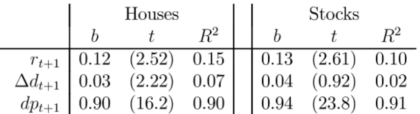
Since houses are so much in the news, Figure 2 shows house prices and rents, and Table III presents a regression. High prices relative to rents mean low returns, not higher subsequent rents, or prices that rise forever. The housing regressions are almost the same as the stock market regressions. (Not everything about house and stock data is the same of course. Measured house price data are more serially correlated.)
Houses Stocks
2 2
+1 0.12 (2.52) 0.15 0.13 (2.61) 0.10
∆+1 0.03 (2.22) 0.07 0.04 (0.92) 0.02 +1 0.90 (16.2) 0.90 0.94 (23.8) 0.91
Table III. Left: Regressions of log annual housing returns+1, log rent growth
∆+1 and log rent/price ratio +1 on the rent/price ratio , +1 = + ×++1 1960-2010. Right: Regressions of log stock returns +1, dividend
growth ∆+1 and dividend yields +1 on dividend yields , annual CRSP
value weighted return data 1947-2010. 6Fama and French (1988), (1989).
7Fama and Bliss (1987), Campbell and Shiller (1991), Piazzesi and Swanson (2008). 8Fama (1986), Duffie and Berndt (2011).
9Hansen and Hodrick (1980), Fama (1984). 10Gourinchas and Rey (2007).
1960 1970 1980 1990 2000 2010 6.8 7 7.2 7.4 7.6 7.8 20 x Rent Price Date log scale 20 x rent CSW price OFHEOprice
Figure 2: House prices and rents. OFHEO is the Office of Federal Housing Enterprise Oversight "purchase-only" price index. CSW are Case-Shiller-Weiss price data. Data from http://www.lincolninst.edu/subcenters/land-values/rent-price-ratio.asp
There is a strong common element and a strong business cycle association to all these forecasts.11 Low prices and high expected returns hold in “bad times,” when consumption, output and investment are low, unemployment is high, businesses are failing, and vice versa. These facts bring a good deal of structure to the debate over “bubbles” and “excess volatility.” High valuations correspond to low returns, and associated with good economic conditions. All a “price bubble” can possibly mean now is that the equivalent discount rate is “too low” relative to some theory. Regressions do not establish causality. But this equivalence channels us to a much more profitable discussion.
D. The multivariate challenge
This empirical project has only begun. We see that one variable at a time forecasts one return at a time. We need to understand their multivariate counterparts, on both the left and right hand sides of the regressions.
For example the stock and bond regressions on dividend yield and yield spread () are
stock+1 = +×++1 bond+1 = + ×++1
We have some additional predictor variables , from similar univariate or at best bivariate 11Fama and French (1989).
(hence [+×]) explorations,
stock+1 = [+×] +×++1
First, then, which of these variables are really important in a multiple regression sense? In particular, do the variables that forecast one return forecast another?
stock+1 = +×+ × + 0 ++1? (6) bond+1 = + × +×+ 0 ++1?
(I put the variables we need to learn about in boxes.)
Second, how correlated are the right-hand terms of these regressions? What is thefactor structure of time-varying expected returns? Expected returns (+1) vary across time ;
how correlated is such variation across assets and asset classes, and how can we best express that correlation as factor structure? As an example to clarify the question, suppose wefind the stock return coefficients are all double those of the bonds,
stock+1 = + 2×+ 4×++1 bond+1 = + 1×+ 2×++1
We would see a one-factor model for expected returns, with stock expected returns always changing by twice bond expected returns,
¡ stock+1 ¢ = 2×factor (7) ¡ bond+1 ¢ = 1×factor.
Third, we need to relate time-varyingexpected returns to covariances with pricing factors or portfolio returns.
¡
+1¢=(+1f0+1)λ
As a small step down this road, Cochrane and Piazzesi (2005) (2008) find that forward rates ofall maturities help to forecast returns ofeach maturity — multiple regressions matter as in (6). We found that the right-hand sides are almost perfectly correlated across left-hand maturities.12 A single common factor describes 99.9% of the variance ofexpected returns as in
(7). Finally, wefind that the spread in time-varying expected bond returns across maturities corresponds to a spread in covariances with a single “level” factor, and the market prices of risk of slope, curvature, and expected-return factors are zero.
What similar patterns hold across broad asset classes? The challenge, of course, is that there are too many right hand variables, so we can’t just go run huge multiple regressions. But these are the vital questions.
E. Multivariate prices
I advertised much of the point of running return regressions with prices on the right hand side was to understand those prices. How will a multivariate investigation change our picture of prices and long-run returns?
Again, the Campbell-Shiller present value identity
≈ ∞ X =1 −1+ − ∞ X =1 −1∆+ (8)
provides a useful way to think about these questions. Since this identity holds ex-post, it holds for any information set. Dividend yields are a great forecasting variable because they reveal market expectations of dividend growth and returns. However, dividend yields combine the two sources of information. A variable can help the dividend yield to forecast long-run returns if it also forecasts long-run dividend growth. A variable can also help to predictone year returns+1 without much changing long-run expected returns, if it has an
offsetting effect on longer-run returns {+}. Such a variable signals a change in the term
structure of risk premia {+}.
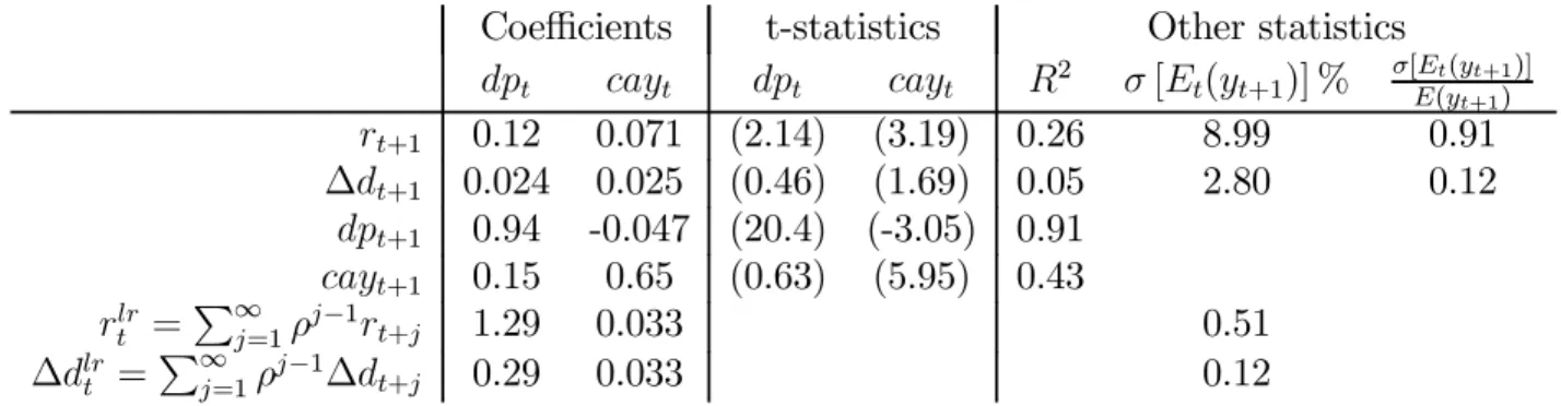
I examine Lettau and Ludvigson’s (2001a) (2005) consumption to wealth ratio cay as an example to explore these questions. Table IV presents forecasting regressions
Coefficients t-statistics Other statistics
2 [(+1)] % [((+1)] +1) +1 0.12 0.071 (2.14) (3.19) 0.26 8.99 0.91 ∆+1 0.024 0.025 (0.46) (1.69) 0.05 2.80 0.12 +1 0.94 -0.047 (20.4) (-3.05) 0.91 +1 0.15 0.65 (0.63) (5.95) 0.43 = P∞ =1−1+ 1.29 0.033 0.51 ∆ = P∞ =1 −1∆ + 0.29 0.033 0.12
Table IV. Forecasting regressions using dividend yield and consumption-wealth ratio, 1952-2009, annual data. Long-run coefficients are computed using a first-order VAR with and as state variables. Each regression includes a constant. Cay is rescaled so() = 1. () = 042.
Cay helps to forecast one-period returns. The t statistic is large, and it raises the variation of expected returns substantially. Cay only marginally helps to forecast dividend growth. (Lettau and Ludvigson report that it works better in quarterly data.)
Figure 3 graphs the one-year return forecast using dp alone, the one-year return forecast using dp and cay together, and the actual ex-post return. Adding cay lets us forecast business-cycle frequency “wiggles” while not much changing the “trend.”
1950 1960 1970 1980 1990 2000 2010 −20 −10 0 10 20 30 40 dp and cay dp only actual r t+1
Figure 3: Forecast and actual 1 year returns. The forecasts are fitted values of regressions of returns on dividend yield and cay. Actual returns are plotted on the same date as their forecast, i.e. +1 is plotted at the same date as +×.
1950 1960 1970 1980 1990 2000 2010 −5 −4.5 −4 −3.5 −3 −2.5 E(rlr|dp,cay) E(rlr|dp) dp
Figure 4: Dividend yield dp and forecasts of long-run returnsP∞=1−1
+Return forecasts are computed from a VAR including dp, and a VAR including dp and cay.
Long-run return forecasts are quite different. Figure 4 contrasts long-run return forecast with and without cay. Though cay has a dramatic effect on one-period return+1 forecasts
in Figure 3, cay has almost no effect at all on long-run return P∞=1−1
+ forecasts in Figure 4.
Figure 4 includes the actual dividend yield, to show (by (8)) how dividend yields break into long-run return vs. dividend growth forecasts. The last two rows of Table IV give the corresponding long-run regression coefficients. Essentially all price-dividend variation still
corresponds to expected-return forecasts.
How can cay forecast one-year returns so strongly, but have such a small effect on the terms of the dividend-yield present value identity? In the context of (8), cay alters theterm structure of expected returns.
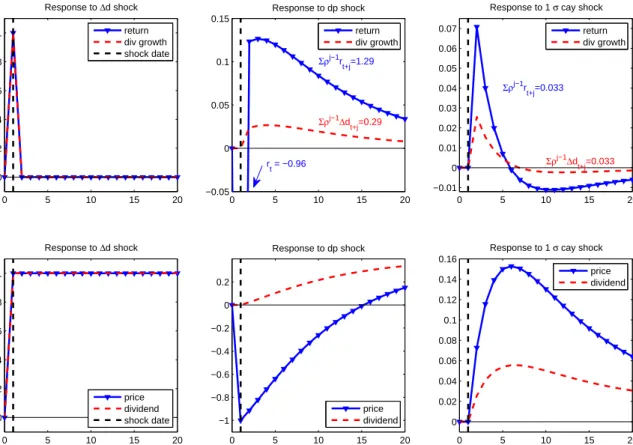
We can display this behavior with impulse-response functions. Figure 5 plots responses to a dividend growth shock, a dividend yield shock, and a cay shock. In each case, I include a contemporaneous return response to satisfy the return identity+1 =∆+1−+1+.
0 5 10 15 20 0 0.2 0.4 0.6 0.8 1 Response to Δd shock return div growth shock date 0 5 10 15 20 −0.05 0 0.05 0.1 0.15 Response to dp shock Σρj−1r t+j=1.29 Σρj−1Δd t+j=0.29 rt = −0.96 return div growth 0 5 10 15 20 −0.01 0 0.01 0.02 0.03 0.04 0.05 0.06 0.07
Response to 1 σ cay shock
Σρj−1 rt+j=0.033 Σρj−1Δd t+j=0.033 return div growth 0 5 10 15 20 0 0.2 0.4 0.6 0.8 1 Response to Δd shock price dividend shock date 0 5 10 15 20 −1 −0.8 −0.6 −0.4 −0.2 0 0.2 Response to dp shock price dividend 0 5 10 15 20 0 0.02 0.04 0.06 0.08 0.1 0.12 0.14 0.16
Response to 1 σ cay shock
price dividend
Figure 5: Response functions to dividend growth, dividend yield, and cay shocks. Cal-culations are based on the VAR of Table 4. Each shock changes the indicated vari-able without changing the others, and includes a contemporaneous return shock +1 =
∆+1−+1+. The vertical dashed line indicates the period of the shock.
These plots answer the question, “what change in expectations corresponds to the given shock?” The dividend growth shock corresponds to permanently higher expected dividends with no change in expected returns. Prices jump to their new higher value and stay there. It is a pure “expected cashflow” shock. The dividend yield shock is essentially a pure discount rate shock. It shows a rise in expected returns with little change in expected dividend growth. The cay shock in the rightmost panel of Figure 5 corresponds to a shift in expected returns from the distant future to the near future, with a small similar movement in the timing of a dividend growth forecast. It has almost no effect on long run returns or dividend
growth. We could label it a shock to the term structure of risk premia.13
So, cay strongly forecasts one-year returns, but has little effect on price-dividend ratio variance attribution. Does this pattern hold for other return forecasters? I don’t know. In principle, consistently with the identity (8), other variables can help dividend yields to predict both long-run returns and long-run dividend growth. Consumption and dividends should be cointegrated, and since dividends are so much more volatile, the consumption-dividend ratio should forecast long-run consumption-dividend growth. Cyclical variables should work: at the bottom of a recession, both discount rates and expected growth rates are likely to be high, with offsetting effects on dividend yields. Reflecting both ideas, Lettau and Ludvigson (2005) report that “cdy” a cointegrating vector including dividends, does forecast long-run dividend growth in just this way. However, the lesser persistence of typical forecasters will work against much effect on price-dividend ratios. Cay’s coefficient of only 0.65 on its own lag, and the fact that cay did not forecast dividend yields, are much of the story for cay’s failure to affect long-run forecasts.
Even so, if additional variables help to forecast long-run dividend growth, they can only
raise the contribution of long-run expected returns to price-dividend variation. It does not shift variance attribution from returns do dividends. A higher long-run dividend forecast must be matched by a higher long-run return forecast if it is not to affect the dividend yield. This is a suggestivefirst step, not an answer. We have a smorgasbord of return forecasters to investigate, singly and jointly, including information in additional lags of returns and dividend yields (see the Appendix). The point is this: Multivariate long-run forecasts and consequent price implications can be quite different from one-period return forecasts. As we pursue the multivariate forecasting question using the large number of additional forecasting variables, we should look at pricing implications, not just focus on short-run 2 contests.
III. The Cross Section
In the beginning, there was chaos; practitioners thought one only needed to be clever to earn high returns. Then came the CAPM. Every clever strategy to deliver high average returns ended up delivering high market betas as well. Then anomalies erupted, and there was chaos again. The “value effect” was the most prominent anomaly.
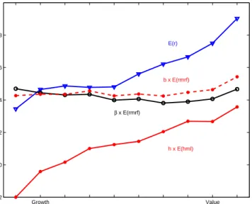
Figure 6 presents Fama-French 10 book/market-sorted portfolios. Average excess returns rise from growth (low book/market, “high price”) to value (high book/market, “low price”). This fact would not be a puzzle if the betas also rose. But the betas are about the same for all portfolios.
The absence of beta is really the heart of the value puzzle. It’s perfectly natural that stocks which have fallen on hard times should have higher subsequent returns. If the market declines, these stocks should be particularly hard hit. They should have higher average returns — and higher betas. All puzzles are joint puzzles of expected returns and betas. Beta without expected return is just as much a puzzle — and profitable — as expected return
without beta.14
Fama and French (1993), (1996) brought order once again with size and value factors. Figure 6 includes the results of multiple regressions on the market and Fama and French’s hml factor,
=+×+×+
The Figure shows the separate contributions of×()and×()in accounting for average returns(). Higher average returnsdo line up well with larger values of the
regression coefficient
Growth Value −0.2 0 0.2 0.4 0.6 0.8 E(r) β x E(rmrf) b x E(rmrf) h x E(hml) Average return
Average returns and betas
Figure 6: Average returns and betas for Fama - French 10 Book/Market sorted portfolios. Monthly data 1963-2010.
Fama and French’s factor model accomplishes a very useful data reduction. Theories now only have to explain the hml portfolio premium, not the expected returns of individual assets.15 This lesson has yet to sink in to a lot of empirical work, which still uses the 25 Fama French portfolios to test deeper models.
Covariance is in a sense Fama and French’s central result: if the value firms decline, they all decline together. It’s a sensible result: Where there is mean, there must be comovement, so that Sharpe ratios do not rise without limit in well-diversified value portfolios.16 But
theories now must also explain thiscommon movement among value stocks. It is not enough to simply generate temporary price movements, a “fad” that produces high or low prices, and then fades away rewarding contrarians. You need all the low-price securities to subsequently
rise and fall together in the following month.
Finally, Fama and French found that other sorting variables, such as firm sales growth, did not each require a new factor. The three-factor model took the place of the CAPM for
14Frazzini and Pedersen (2010).
15Daniel and Titman (2006), Lewellen, Nagel, and Shanken (2010). 16Ross (1976), (1978).
routine risk-adjustment in empirical work.
Order to chaos, yes, but once again, the world changed 100%. None of the cross-section of average stock returns corresponds to market betas. 100% corresponds to (and size) betas.
Alas, the world is once again descending into chaos. Expected return strategies have emerged that do not correspond to market, value, and size betas. These include, among many others, momentum17, accruals, equity issues and other accounting-related sorts,18 beta
arbitrage, credit risk, bond and equity market-timing strategies, foreign exchange carry trade, put option writing, and various forms of “liquidity provision.”
A. The multidimensional challenge
We’re going to have to repeat Fama and French’s anomaly digestion, but with many more dimensions. We have a lot of questions to answer:
First, which characteristics really provide independent information about average re-turns? Which are subsumed by others?
Second, does each new anomaly variable also correspond to a new factor formed on those same anomalies? Momentum returns correspond to regression coefficients on a winner-loser momentum “factor.” Carry-trade profits correspond to a carry-trade factor.19 Do accruals
return strategies correspond to an accruals factor? We should routinely look.
Third, how many of these new factors are really important? Can we again account for
independent dimensions of expected returns with factor exposures? Can we account for accruals return strategies by betas on some other factor, as with sales growth?
Now, factor structure is neither necessary nor sufficient for factor pricing. ICAPM and consumption-CAPM models do not predict or require that the multiple pricing factors will correspond to big common movements in asset returns. And big common movements, such as industry portfolios, need not correspond to any risk premium. There always is an equivalent single-factor pricing representation of any multifactor model, the mean-variance efficient portfolio. Still, the world would be much simpler if betas on only a few factors, important in the covariance matrix of returns, accounted for a larger number of mean characteristics.
Fourth, eventually, we have to connect all this back to the central question of finance, why do prices move?
B. Asset pricing as a function of characteristics/uni
fi
cation
To address these questions in the zoo of new variables, I suspect we will have to use different
methods. Following Fama and French, a standard methodology has developed: sort assets into portfolios based on a characteristic, look at the portfolio means, especially the 1-10 portfolio
17Jegadeesh and Titman (1993). 18See Fama and French (2010).
alpha, information ratio, and t-statistic, and then see if the spread in means corresponds to a spread of portfolio betas against some factor. But we can’t do this with 27 variables.
Portfolio sorts are really the same thing as nonparametric cross sectional regressions, using rather inefficient non-overlapping histogram weights. Figure 7 illustrates the point. For one variable, portfolio sorts and regressions both work. But we can’t chop portfolios 27
Log(Book/market) E(R) 1 2 3 4 5 Portfolio Portfolio Mean Securities Better weights?
Figure 7: Portfolio means vs. cross -sectional regressions.
ways, so I think we will end up running multivariate regressions.20 (The Appendix gives a simple cross-sectional regression to illustrate.)
Having said that, you see that “time series” forecasting regressions, “cross-sectional” regressions and portfolio mean returns are really the same thing. All we are ever really doing is understanding a big panel-data forecasting regression
+1 =+0++1
We end up describe expected returns as a function of characteristics,
(+1|) where C denotes some big vector of characteristics,
= [size, b/m, momentum, accruals, d/p, credit spread....]
Is value a “time-series” strategy that moves in and out of a stock as that stock’s book/market changes, or a “cross-sectional” strategy that moves from one stock to another following the same signal? Well, both, obviously. They are the same thing. This is the managed-portfolio theorem:21 an instrument
in a time series test 0 =
£¡ +1+1 ¢ ¤ is the same as an unconditional test of a managed portfolio0 =£+1
¡
+1
¢¤
.
Once we understand expected returns, we have to see if expected returns line up with covariances of returns with factors. Sorted-portfolio betas are a nonparametric estimate of 20Fama and French (2010) already run such regressions, despite evident reservations over functional forms. 21Cochrane (2005c).
this covariance function
(+1 +1) =()
Parametric approaches are natural here as well, to address a multidimensional world. For example, we can run regressions
£
+1−(+1|)
¤
+1 =+0++1 ⇒() =+0
(The errors may not be normal, but they are mean-zero and uncorrelated with the right hand variable.) We want to see if the mean return function lines up with the covariance
function.
(|) =()×?
Underlying everything we’re doing is an assumption that expected returns, variances and covariances are stable functions of characteristics, not (say) security name. That’s why we use portfolios in the first place. That is an incredibly useful assumption—or, fact about the world. Without it, it’s hard to tell if there is any spread in average returns at all. It means however, that asset pricing really is about the equality of twofunctions; the function relating means to characteristics and the function relating covariance to characteristics.
Looking at portfolio average returns rather than forecasting regressions was really the key to understanding economic importance of many effects, as was looking at long-horizon returns. For example, serial correlation with an2 of 0.01 doesn’t seem that impressive. Yet is enough to account for momentum: The last year’s winners went up 100%, so an annual autocorrelation of 0.1, meaning 0.01 2, generates a 10% annual portfolio mean return.
(An even smaller amount of time-series cross-correlation works as well.) As another classic example, Lustig, Roussanov, and Verdelhan (2010a) translated carry-trade return-forecasting regressions to means of portfolios formed on the basis of currency interest differentials. This step led them to look for and find a factor structure of country returns that depends on interest differentials, a “high minus low” factor. This step followed Fama and French (1996) exactly, but no one thought to look for it in 30 years of running country-by-country time-series forecasting regressions
But the equivalence of portfolio sorts and regressions goes both ways. We can still calcu-late these measures of economic significance if we estimate panel-data regressions for means and covariances. From the spread of lagged returns, we can calculate the momentum portfo-lio implications directly. The 1-10 portfoportfo-lio information ratio is the same thing as the Sharpe ratio of the underlying factor, or t-statistic of the cross-sectional regression coefficient. (See the Appendix.) We could study the covariance structure of panel-data regression residuals as a function of the same characteristics (interest rate spread, for example) rather than actually form portfolios,
(+1
+1) =( )
Running multiple panel-data forecasting regressions is full of pitfalls of course. One can end up focusing on tiny firms, or outliers. One can get the functional form wrong. Uniting time-series and cross section will yield new insights as well. For example, variation in book/market over time for a given portfolio has a larger effect on returns than variation
in book/market across the Fama-French portfolios, and a recent change in book/market also seems to forecast returns. (See the Appendix.) I didn’t say it will be easy! But we must address the factor zoo, and I don’t see how to do it by a high-dimensional portfolio sort.
C. Prices
Then, we have to answer the central question, what is the source of price variation?
When did our field stop being “asset pricing” and become “asset expected returning?” Why are betas exogenous?22 A lot of price variation comes from discount factor news. What sense does it make to “explain” expected returns by the covariation of expected return shocks with market expected return shocks? Market/book ratios should be our left-hand variable, the thing we’re trying to explain, not a sorting characteristic for expected returns.
Focusing on expected returns and betas rather than prices and discounted cashflows makes sense in a two-period or i.i.d. world, since in that case betas are all cashflow betas. It makes much less sense in a time-varying discount rate world.
A long-run, price-and-payoffperspective may also end up being simpler. As a hint of the possibility, solve the Campbell-Shiller identity for long-run returns,
∞ X =1 −1+ = ∞ X =1 −1∆+−
So,long-run return uncertainty all comes from cashflow uncertainty. Long-run betas are all cashflow betas. The long run looks just like a simple one-period model with a liquidating dividend. +1 = +1 = µ +1 ¶ µ ¶ +1 = ∆+1−
A natural start is to forecast long-run returns and form price decompositions in the cross section, just as in the time-series; estimate forecasts such as
∞
X
=1
−1+ =+0+
and then understand valuations with present value models as before.23 (The Appendix
includes two simple examples.)
In a formal sense, of course, it doesn’t matter whether you look at returns or prices.
1 =(+1+1) and =
P∞
=1++ each imply the other. But, as I found with return forecasts, our economic understanding may be a lot different in a price, long-run
22Campbell and Mei (1993).
view than focusing on short-run returns. What constitutes a “big” or “small” error is also different if we look at prices vs. returns. At a 2% dividend yield, = (−) implies that an “insignificant” 10bp/month expected return error is a “large” 12% price error, if it is permanent. For example, since momentum amounts to a very small time-series correlation and lasts less than a year, I suspect it has little effect on long-run expected returns and hence the level of stock prices. Long-lasting characteristics are likely to be more important. Conversely, small transient price errors can have a large impact on return measures. A tiny i.i.d. price error induces the appearance of mean reversion where there is none. Common procedures amount to taking many differences of prices, which amplify the error/signal ratio. For example, the forward spread()−
(1) = (−1) − () + (1)
is already a triple-difference of price data.
IV. Theories
Having viewed a bit of how discount rates vary, Let’s think now about why discount rates vary so much.
A. A categorization, by ingredients and connection to data
It’s useful to classify theories by their main ingredient, and by which data they use to measure discount rates. My goal is to produce for discount rates something like Fama’s (1970) classification of informational possibilities.
1. Theories based on fundamental investors, with few frictions. (a) Macroeconomics — tie to macro data.
i. Consumption, Aggregate risks.
ii. Risk sharing/background risks (Hedging outside income) iii. Investment and production.
iv. General equilibrium, including macroeconomics
(b) Behavioral; Irrational expectations. Tie to price data. Other data?
(c) Finance. Expected return-beta, return-based factors, affine term structure mod-els. Tie to price data, returns explained by covariances.
2. Theories based on frictions.
(a) Segmented markets — different investors in different markets; limited risk bearing of active traders.
(b) Intermediated markets. Prices set by leveraged intermediaries; funding difficulties. (c) Liquidity.
i. Idiosyncratic — easy to sell the asset. ii. Systemic — times of market illiquidity.
iii. Information trading — value of securities in facilitating information trading. “Macro” theories tie discount rates to macroeconomic data, such as consumption or investment, based on first-order conditions for the ultimate investors or producers.
For example, the canonical consumption-based model with power utility relates discount rates to consumption growth,
+1 = (+ 1) () = µ +1 ¶− ; (+1) = ( +1 +1)≈(+1∆+1)
High expected returns (low prices) correspond to securities that pay off poorly when con-sumption is low. This model combines frictionless markets, rational expectations and utility maximization, and risk sharing so that only aggregate risks matter for pricing. It evidently ties discount rate variation to macroeconomic data.
A vast literature has generalized this framework, including (among others)24 1)
Nonsepa-rability across goods — durable and nondurable25; traded and nontraded; 2) Nonseparability over time, such as habit persistence,26 3) Recursive utility and long-run risks27 4) Rare
disasters, which alter measurements of means and covariances in “short” samples28.
A related category of theories adds incomplete markets or frictions preventing some consumers from participating. Though they include “frictions,” I categorize such models here because asset prices are still tied to some fundamental consumer or investor’s economic outcomes. For example, if non-stockholders do not participate, we still tie asset prices to the consumption decisions of stockholders who do participate.29
With incomplete markets, consumers still share risks as much as possible. The complete-market theorem that “all risks are shared,” marginal utility is equated across peopleand,
+1 =
+1, becomes “all risks are shared as much as possible.” The projection of marginal
utility on asset payoffs is the same across people(
+1|) =(
+1|)≡∗. We
can still aggregate marginal utility rather than aggregate consumption before constructing marginal utility. A discount factor +1 =+1(+1) =
R
()+1 prices assets, where +1 takes averages across people conditional on aggregates. For example with power utility
we have +1 =+1 "µ +1 ¶−#
24See Cochrane (2007a), Ludvigson (2011) for recent reviews. 25Recently, Yogo (2006),
26Campbell and Cochrane (1999) for example.
27Epstein and Zin (1989), Bansal and Yaron (2004), Hansen, Heaton and Li (2008). 28Rietz (1988), Barro (2006).
The fact that we aggregate nonlinearly across people means that variation in thedistribution
of consumption matter to asset prices. Times in which there is morecross-sectional risk will be high-discount factor events.30
Outside or nontradeable risks are a related idea. If a mass of investors has jobs or businesses that will be hurt especially hard by a recession, they avoid stocks that fall more than average in a recession.31 Average stock returns then reflect the tendency to fall more
in a recession, in addition to market risk exposure. Though in principle, given a utility function, one could see such risks in consumption data, individual consumption data will always be so poorly measured that tying asset prices to more fundamental sources of risk may be more productive.
If we ask the “representative investor” in December 2008 why he or she is ignoring the high premiums offered by stocks and especiallyfixed income, the answer might well be “that’s nice, but I’m about to lose my job, and my business might go under. I can’t take any more risks right now, especially in securities that will lose value or become hard to sell if the recession gets worse.” These extensions of the consumption-based model all formalize this sensible intuition — as opposed to the idea that these consumers have wrong expectations, or that they would have been happy to take risks but intermediaries were making all asset pricing decisions for them.
Investment-based models link asset prices tofirms investment decisions, and general equi-librium models include production technologies and a specification of the source of shocks. This is clearly the ambitious goal towards which we are all aiming. The latter tries to answer the vexing questions, where do betas come from? What makes a company a “growth” or “value” company in the first place?32
I think “behavioral” asset pricing’s central idea is that people’s expectations are wrong.33 It takes lessons from psychology to find systematic patterns to the “wrong” expectations. There are some frictions in many behavioral models, but these are largely secondary and defensive, to keep risk-neutral “rational arbitrageurs” from coming in and undoing the be-havioral biases. Often, simple risk aversion by the rational arbitrageurs would serve as well. Behavioral models, like “rational” models, tie asset prices to the fundamental investor’s willingness, ability or (in this case) perception of risk.
Behavioral theories are also discount-rate theories. A distorted probability with riskfree discounting is mathematically equivalent to a different discount rate.
=X = 1 X ∗ where ∗ ≡ = X 0 00 30Constantinides and Duffie (1996) .
31Fama and French (1996), Heaton and Lucas (2000).
32A few good examples: Gomes, Kogan and Zhang (2003), Gala (2010), Gourio (2007).. 33See Barberis and Thaler (2003) and Fama (1998) for reviews.
denote states of nature, are true probabilities, is a stochastic discount factor or marginal utility growth, and ∗
are distorted probabilities.
It is pointless to argue “rational” vs. “behavioral” in the abstract. There is a dis-count rate and equivalent distorted probability that can rationalize any (arbitrage-free) data. “The market went up, risk aversion must have declined” is as vacuous as “the market went up, sentiment must have increased.” Any model only gets its bite by restricting discount rates or distorted expectations, ideally tying them to other data. The only thing worth arguing about is how persuasive those ties are in a given model and dataset, and whether it would have been easy for the theory to “predict” the opposite sign if the facts had come out that way.34 And the line between recent “exotic preferences” and “behavioral finance” is so
blurred35 it describes academic politics better than anything substantive.
A good question for any theory is what data it uses to tie down discount factors. By and large, behavioral research so far largely ties prices to other prices; it looks for price patterns that are hard to understand with other models, such as “overreaction” or “under-reaction” to news. Some behavioral research uses survey evidence, and survey reports of people’s expectations are certainly unsettling. However, surveys are sensitive to language and interpretation. It doesn’t take long in teaching MBAs to realize that the colloquial meanings of “expect” and “risk” are entirely different from conditional mean and variance. If people report therisk-neutral expectation, then expectations are in fact completely ratio-nal. An “optimistic” cash-flow growth forecast is the same as a “rational” forecast, already discounted at a low rate, and leads to the correct decision, invest more. And the risk-neutral expectation, i.e. the expectation weighted by marginal utility, is the right sufficient statistic for many decisions. Treat painful things as if they were more probable than they are in fact. Of course, “rational” theories beyond the simple consumption-based model struggle as well. Changing expectations of consumption 10 years from now (long run risks) or chang-ing probabilities of a big crash are hard to tell from changchang-ing “sentiment.” At least, one can aim for more predictions than assumptions, tying together several phenomena with a parsimonious specification.
“Finance” theories tie discount rates to broad return-based factors. That’s great for data reduction and practical applications. The more practical and “relative-pricing” the application the more “factors” we accept on the right hand side. For example, in evaluating a portfolio manager, hedging a portfolio, orfinding the cost of capital for a given investment we routinely include momentum as a “factor” even though we don’t have a deep theory of why the momentum factor is priced.
However, we still need the deeper theories for deeper “explanation.” Even if the CAPM explained individual mean returns from their betas and the market premium, we would still have the equity premium puzzle — why is the market premium so large? (And why are betas what they are?) Conversely, even if we had the perfect utility function and a perfect consumption-based model, the fact that consumption data is poorly measured means we
34Fama (1998).
35For example, which of Epstein and Zin (1989), Barberis, Santos, and Huang (2001), Hansen and Sargent
(2005), Laibson (1997), Hansen, Heaton and Li (2008), and Campbell and Cochrane (1999) is really “rational” and which is really “behavioral?”
would still use finance models for most practical applications.36
A nice division of labor results. Empirical asset pricing in the Fama and French (1996) tradition boils down the alarming set of anomalies to a small set of large-scale systematic risks that generate rewards. “Macro” “behavioral” or other “deep” theories can then focus on why the factors are priced.
Models that emphasize frictions are becoming more and more popular, especially since the financial crisis. At heart, these models basically maintain the “rational” assumption. Admittedly, there are often “irrational” agents in such models. However, these agents are usually just convenient shortcuts rather than central to the vision. A model may want some large volume of trade,37 or to include some “noise traders,” while focusing clearly on the
delegated management problem, or the problem of leveraged intermediaries. For such a purpose, it’s easy to simply allude to a slightly irrational class of trader rather than spell out their motives from first principles. However those assumptions are not motivated by deep reading of psychology or lab experiments. The focus is on the frictions and behavior of intermediaries rather than the risk-bearing ability of ultimate investors, or their psychological misperceptions.
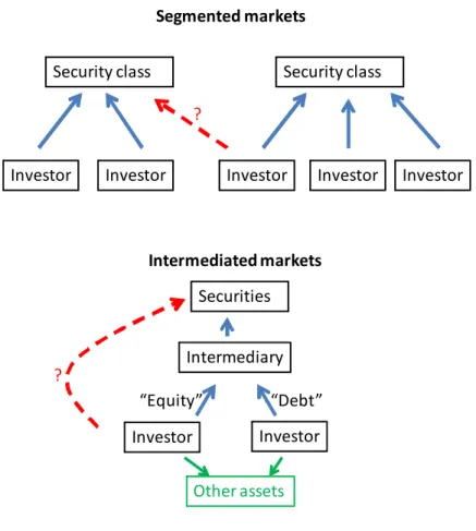
I think it’s useful to distinguish three categories of frictions: 1) Segmented markets and 2) Intermediated markets or “institutional finance”38 and 3) Liquidity.
I distinguish “segmented markets” from “intermediated markets,” as shown in Figure 8. Segmentation is really about limited risk sharing among the pool of investors active in a particular market.39 They can generate “downward sloping demands,” and average returns that depend on a “local” factor, little and poorly-linked CAPMs.40 Given the factor zoo,
that’s an attractive idea.
“Intermediated markets” or “institutional finance” refers to a different, vertical rather than horizontal, separation of investor from payoff. Investors use delegated managers. Then, agency problems in delegated management spill over into asset prices. For example, suppose investors split their investments to the managers into “equity” and “debt” claims. When losses appear, the managers stave offbankruptcy by trying to sell risky assets. But since all the managers are doing the same thing, prices fall and discount rates rise. Colorful terms like “fire sale,” “liquidity spirals” describe this process.41
Of course, we have to document and explain segmentation and intermediation. As sug-gested by the dashed arrows in Figure 8, there are strong incentives to undo any price anomaly induced by segmentation or intermediation. Models with these frictions often ab-stract from deep-pockets unintermediated investors — the sovereign wealth funds, pension funds, endowments, family offices, and Warren Buffets, or institutional innovation to bridge
36Campbell and Cochrane (2000) give a quantitative example. 37Scheinkman and Xiong (2003).
38Markus Brunnermeier coined this useful term.
39Some important examples: Burnnermeier and Pedersen (2009), Brunnermeier (2009), Gabaix,
Krishna-murthy and Vigneron (2007), Duffie and Strulovici (2011), Garleanu and Pedersen (2009), He and Krishna-murthy (2010), KrishnaKrishna-murthy (2008), Froot and O’Connell (2008), Vayanos and Vila (2011).
40For example, Gabaix, Krishnamurthy and Vigneron (2007).
Investor Investor Investor Security class Investor Investor Investor Investor Intermediary “Debt” “Equity” ? ? Other assets Segmented markets Intermediated markets Security class Securities
Figure 8: Segmented markets vs. intermediated markets.
the friction. Your “fire sale” is their “buying opportunity.” Thus, I think a little more attention to the reasons for segmentation and intermediation will help to define when and how long these models apply. For example, transactions costs, attention costs, or limited expertise suggest markets can be segmented until the “deep pockets” arrive, but that they do arrive eventually. So if this is why markets are segmented, that segmentation will be more important in the short run, after unusual events, or in more obscure markets. If I try to sell a truckload of tomatoes at 2 am in front of the Booth school, I am not likely to get full price. But if I do it every night, tomato buyers will start to show up. In the flash crash, it took about ten minutes for buyers to show up, which is either remarkably long or remarkably short, depending on your point of view.
A crucial question is, as always, what data will this class of theories use to measure dis-count rates? Arguing over puzzling patterns of prices is weak (the rational-behavioral debate has been doing that for 40 years). Ideally, one should tie price or discount-rate variation to central items in the models, such as the balance sheets of leveraged intermediaries, data on who is actually active in segmented markets, and so forth. Yet such data is hard to find.42
42Mitchell, Pedersen and Pulvino (2007) is a good example. They document who was active in convertible
arbitrage markets through two episodes in which the specialized hedge funds left the market and it took months for the multi-strategy funds to move in.
We have long recognized that some assets have higher or lower discount rates in compen-sation for greater or lesser liquidity.43 We have also long struggled to define and measure
liquidity. There are (at least) three kinds of stories for liquidity that are worth distinguish-ing. Liquidity can refer to the ease of buying and selling an individual security. Illiquidity can also be systemic: assets will face a higher discount rate if their prices fall when the market as a whole is illiquid, whether or not the asset becomes more or less illiquid. Fi-nally, assets can have lower discount rates if they facilitate information trading, as money facilitates physical trading.
I think of “liquidity” as different from “segmentation” in that segmentation is about limited risk-bearing ability, while liquidity is about trading. Liquidity is a feature of assets, not the risks to which they are claims. Many theories of liquidity emphasize asymmetric information, not limited risk-bearing ability — assets become illiquid when traders suspect that anyone buying or selling knows something, not because traders are holding too much of a well-understood risk. Understanding liquidity requires us to unravel the puzzle of why people and institutions trade so vastly more than they do in our models.
All of these facts and theories are really about discount rates, expected returns, risk bearing, risk sharing and risk premiums. None are fundamentally about slow or imperfect diffusion of cash-flow information, i.e. informational “inefficiency.” Informational efficiency isn’t wrong or disproved. Efficiency basically won, and we moved on. When we see infor-mation, it is quickly incorporated in asset prices. There is a lot of asset-price movement not related to visible information, but Hayek (1945) told us that would happen, and we learned that a lot of such price variation corresponds to expected returns. Little of the (large) gulf between the above models is really about information. Seeing the facts and the models as categories of discount-rate variation seems much more descriptive of most (not all) theory and empirical work.
Informational efficiency is much easier for markets and models to obtain than wide risk sharing or desegmentation, which is perhaps why it holds more broadly. A market can become efficient with only one informed trader, who doesn’t need to actually buy anything or take any risk. He should run in to a wall of indexers, and end up just bidding up the asset he knows is underpriced.44 Though price discovery seems in reality to come with a lot of
trading, it doesn’t have to do so. Risk sharing needseveryone to change their portfolios and bear a risk in order to eliminate segmentation. For example, if the small firm effect came from segmentation, the passively-managed small stock fund or total market fund should have ended it — but it also took the invention and marketing of such funds to end it. The actions of small numbers of arbitrageurs could not do so.
B. Recent performance
This is not the place for a deep review of theory and empirical work supporting or confronting theories. Instead, I think it will be more productive to think informally about how these 43Acharya and Pedersen (2005), Amihud, Mendelson and Pedersen (2005), Cochrane (2005b), Pastor and
Stambaugh (2003), Vayanos and Wang (2011).
classes of models might be able to handle big recent events.
C. Consumption
I still think the macro-finance approach is promising. Figure 9 presents the market price-dividend ratio, and aggregate consumption relative to a slow-moving “habit.” The habit is basically just a long moving average of lagged consumption, so the surplus consumption ratio line is basically detrended consumption.45
1990 1992 1995 1997 2000 2002 2005 2007 2010 Surplus consumption (C−X)/C and stocks
SPC (C−X)/C P/D
Figure 9: Surplus consumption ratio and price/dividend ratio. Surplus consumption is formed from real nondurable + services consumption using the Campbell and Cochrane (1999) specification and parameters. Price/dividend ratio is from the CRSP NYSE Value-Weighted portfolio.
As you can see, consumption and stock market prices did both collapse in 2008. Many high average-return-securities and strategies (stocks, mortgage-backed securities, low-grade bonds, momentum, currency carry) collapsed more than low-average-return counterparts. The basic consumption-model logic — securities must pay higher returns, or fetch lower prices, if their values fall more when consumption falls — isn’t drastically wrong.
The habit model captures the idea that people become more risk averse as consumption falls in recessions. As consumption nears habit, people are less willing to take risks that involve the same proportionate risk to consumption. Discount rates rise, and prices fall. Lots of models have similar mechanisms, especially models with leverage.46 In the habit
model, the price-dividend ratio is a nearly log-linear function of the surplus consumption 45Campbell and Cochrane (1999)
ratio. The fit isn’t perfect, but the general pattern is remarkably good, given the hue and cry about how the crisis invalidates all traditional finance.
D. Investment
The Q theory of investment is the off-the-shelf analogue to the simple power-utility model from the producer point of view. It predicts that investment should be low when valuations (market to book) are low, and vice versa,
1 +
= market value
book value = (9)
where =investment and =capital.
19901 1992 1995 1997 2000 2002 2005 2007 2010 1.5 2 2.5 3 3.5 4
Nonres. Fixed I/K and Q
I/K P/(20*D) ME/BE
Figure 10: Investment/capital ratio, price/dividend ratio, and market/book ratio. Invest-ment is real private nonresidential fixed investment. Capital is cumulated from investment with an assumed 10% annual depreciation rate. Price/dividend from CRSP, market/book from Ken French’s website.
Figure 10 contrasts the investment/capital ratio, market/book ratio, and price/dividend ratio. The simple Q theory also links asset prices and investment better than you probably thought, both in the tech boom and the financial crisis.
Many finance puzzles are stated in terms of returns. To make that connection, one can transform (9) to a relation linking asset returns to investment growth. Many return puzzles are mirrored in investment growth as the q theory suggests.47
47Cochrane (1991b), (1996) (2007a), Lamont (2000) Li, Livdan and Zhang (2008), Liu, Whithed and
Q theory also reminds us that supply as well as demand matters in setting asset prices. If capital could adjust freely, stock values would never change, no matter how irrational investors are. Quantities would change instead.
I’m not arguing that consumption or investmentcaused the boom or the crash. Endowment-economy causal intuition does not hold in a production Endowment-economy. Thesefirst-order conditions are happily consistent with a view, for example, that rather small losses on subprime mort-gages were amplified by a run on the shadow banking system and flight to quality,48 which
certainly qualifies as a “friction”. The first-order conditions are consistent with many other views of the fundamental determinants of both prices and quantities. But the graphs do argue that asset prices and discount rates are much better linked to big macroeconomic events than most people think (and vice versa). They suggest another important amplifica-tion mechanism: If people did not become more risk averse in recessions, and if firms could quickly transform empty houses into hamburgers, asset prices would not have declined as much.
I also don’t pretend to have perfect versions of either of these first-order conditions, let alone a full macro model that captures value or the rest of the factor zoo. These are very simple and rejectable models. Each makes a 100% R2 prediction that is easy to formally reject. The point is only that research and further elaboration of these kinds of models, as well as using their basic intuition as an important guide to events, is not a hopeless endeavor.
E. Comparisons
Conversely, I think the other kinds of models, though good for describing particular anom-alies, will have greater difficulty accounting for recent big-picture asset pricing events.
We see a pervasive, coordinated rise in the premium for systematic risk, common across all asset classes, and present in completely unintermediated and unsegmented assets.49 For
example, Figure 11 plots government and corporate rates, and Figure 12 plots the baa-aaa spread with stock prices. You can see a huge credit spread open up and fade away along with the dip in stock prices.
Behavioral ideas — narrow framing, salience of recent experience, and so forth — are good at generating anomalous prices and mean returns in individual assets or small groups. They don’t easily generate this kind of coordinated movement that looks just like a rise in risk premium. They don’t naturally generate covariance either. For example, “extrapolation” generates the slight autocorrelation in returns that lies behind momentum. But why should all the momentum stocks then rise and fall together the next month, just as if they are exposed to a pervasive, systematic risk?
Finance models don’t help, of course, because we’re looking at variation of the factors which they take as given.
48Cochrane (2011)..
20070 2008 2009 2010 2011 1 2 3 4 5 6 7 8 9 10 BAA AAA 20 Yr 5 Yr 1 Yr baa,aaa
Figure 11: BAA, AAA, and Treasury yields.
2007 2008 2009 2010 0.5 1 1.5 2 2.5 3 3.5 4
baa−aaa and stocks
baa−aaa sp500 p/d
Figure 12: D/P, S&P500, BAA-AAA.
Segmented or institutional models aren’t obvious candidates to understand broad market movements. Each of us can easily access stocks and bonds through low-cost indices.
And none of these models naturally describe the strong correlation of discount rates with macroeconomic events. Is it a coincidence that people become irrationally pessimistic when the economy is in a tailspin, and they could lose their jobs, houses, or businesses if systematic events get worse?
Again, macro isn’t everything — understanding the smaller puzzles is important. The point is only thatlooking for macro underpinnings for discount rate variation, through fairly simple models, isn’t as hopelessly anachronistic as many seem to think.
F. Arbitrages?
One of the nicest pieces of evidence for segmented or institutional views is that arbitrage relationships were violated in the financial crisis.50 Unwinding the arbitrage opportunities
required one to borrow dollars, which intermediary arbitrageurs could not do.
Figure 13 gives one example. CDS plus Treasury should equal a corporate bond, and usually does. Not in the crisis.
Feb 07 Jun 07 Sep 07 Dec 07 Apr 08 Jul 08 Oct 08 0 1 2 3 4 5 6 Bond CDS Percent
Figure 13: Citigroup CDS and Bond spreads. Source: Fontana (2010).
Figure 14 gives another example, covered interest parity. Investing in the US vs. investing in Europe and returning the money with forward rates should yield the same thing. Not in the crisis. In both cases, profiting from the arbitrage requires one to borrow dollars, which was difficult in the crisis.
Similar patterns happened in many other markets, including even US treasuries.51 Now,
any arbitrage opportunity is a dramatic event. But in each case here thedifference between the two ways of getting the same cashflow is dwarfed by the overall change in prices. And, though an “arbitrage,” the price differences are not large enough to attract “long only” “deep pocket” money. If your precious cash is in a US money market fund, 20 basis points in the depth of afinancial crisis is not enough to get you to listen to the salesman offering offshore investing with an exchange-rate hedging program.
50See also Fleckenstein, Longstaff, and Lustig (2010), 51Hu, Pan and Wang (2011).
Feb 07 Jun 07 Sep 07 Dec 07 Apr 08 Jul 08 Oct 08 Jan 09 May 09 0 1 2 3 4 5 6 7 swap libor
Figure 14: Three-month Libor and FX swap rate. Source: Baba and Packer (2009).
So maybe it’s possible that the “macro” view still builds the benchmark story of overall
price change, with very interesting spreads opening up due to frictions. At least we have a theory for that. Constructing a theory in which the arbitrage spreads drive the coordinated rise in risk premium seems much harder.
The price of coffee displays arbitrage opportunities across locations at the ASSA meetings. (The AFA gave it away for free downstairs while Starbucks was selling it upstairs.) The arbitrage reflects an interesting combination of transactions costs, short-sale constraints, consumer biases, funding limits, and other frictions. Yet we don’t dream that this fact matters for big-picture variation in worldwide commodity prices.
G. Liquidity premia; trading value
Trading-related liquidity does strike me as potentially important for the big picture, and a potentially important source of the low discount rates in “bubble” events.52
I’m inspired by one of the most obvious “liquidity” premiums: Money is overpriced — lower discount rate — relative to government debt, though they are claims to the same payoff
in a frictionless market. And this liquidity spread can be huge — hundreds of percent in hyperinflations.
Now, money is “special” for its use in transactions. But many securities are “special” in trading. Trading needs a certain supply of their physical shares. We cannot support large trading volumes by recycling one outstanding share at arbitrarily high speed. Even short 52Cochrane (2001), (2003), (2005b), Garber (2000), Krishnamurthy (2002), O’Hara (2008), Scheinkman
sellers must hold a share for some short period of time.
Feb98 Sep98 Mar99 Oct99 Apr00 Nov00 May01 Dec01
50 100 150 200 250 300 350 400 450 500 NYSE NASDAQ NASDAQ Tech
Figure 15: Nasdaq Tech, Nasdaq, and NYSE indeces Source: Cochrane (2003).
Feb98 Sep98 Mar99 Oct99 Apr00 Nov00 May01 Dec01
0 100 200 300 400 500 600 700 800 NYSE NASDAQ NASDAQ Tech Dollar volume
Figure 16: Dollar volume in Nasdaq tech, Nasdaq, and NYSE. Source: Cochrane (2003). When share supply is small, and trading demand is large, markets can drive down the discount rate or drive up the price of highly-traded securities, as they do for money. These effects have long been seen in government bonds, for example in the Japanese “benchmark” effect, the spreads between on-the-run and off-the-run Treasuries, or the spreads between Treasury and agency bonds.53 Could these effects extend to other assets?