Investigating human-perceptual properties of "shapes" using 3D shapes and 2D fonts

Investigating Human-Perceptual

Properties of “Shapes” Using 3D

Shapes and 2D Fonts

Luther Power

This dissertation is submitted for the degree of Doctor of

Philosophy

April 2020

Declaration

This thesis has not been submitted in support of an application for another degree at this or any other university. It is the result of my own work and includes nothing that is the outcome of work done in collaboration except where specifically indicated. Many of the ideas in this thesis were the product of discussion with my supervisor Manfred Lau.

Excerpts of this thesis have been published in the following conference manuscripts and academic publications:

Luther Power and Manfred Lau. Schelling Meshes. SAP, Poster, 2017 [1].

Luther Power and Manfred Lau. Schelling Meshes. Eurographics, Short Paper, 2019.

Abstract

Shapes are generally used to convey meaning. They are used in video games, films and other multimedia, in diverse ways. 3D shapes may be destined for virtual scenes or represent objects to be constructed in the real-world. Fonts add character to an otherwise plain block of text, allowing the writer to make important points more visually prominent or distinct from other text. They can indicate the structure of a document, at a glance.

Rather than studying shapes through traditional geometric shape descriptors, we provide alternative methods to describe and analyse shapes, from a lens of human perception. This is done via the concepts of Schelling Points and Image Specificity.

Schelling Points are choices people make when they aim to match with what they expect others to choose but cannot communicate with others to determine an answer. We study whole mesh selections in this setting, where Schelling Meshes are the most frequently selected shapes. The key idea behind image Specificity is that different images evoke different descriptions; but ‘Specific’ images yield more consistent descriptions than others. We apply Specificity to 2D fonts.

We show that each concept can be learned and predict them for fonts and 3D shapes, respectively, using a depth image-based convolutional neural network. Results are shown for a range of fonts and 3D shapes and we demonstrate that font Specificity and the Schelling meshes concept are useful for visualisation, clustering, and search applications. Overall, we find that each concept represents similarities between their respective type of shape, even when there are discontinuities between the shape geometries themselves. The ‘context’ of these similarities is in some kind of abstract or subjective meaning which is consistent among different people.

Acknowledgements

Firstly, I would like to thank my parents for bringing me into this world, and my Dad especially for inspiring me to become involved in Computing. Luckily my stubbornness didn’t impede me from heeding his advice. I also appreciate the timely assistance of my friends: Callum Shields, Tahsin Rahman and James Buckley, for dragging me away from my work and worries from time to time, to relax – although sometimes engaging in heated political arguments, in the case of Callum – helping me to stay on track with my work and keep a clear mind.

I would also like to thank Dr. Kapil Dev and Aluna Everitt for being brilliant lab colleagues. Their work and determination always encouraged me to keep motivated. I must also mention Dr. John Hardy at this point, who helped me feel welcome during the initial stages of my PhD.

In addition, I would like to thank Lancaster University as a whole, for giving me the opportunity to study for a PhD, via a scholarship. In relation to this, I would like to give thanks to Prof. Hans Gellersen and Dr. Gerald Kotonya for their support. Lastly, I want to acknowledge the great supervision I have had under Dr. Manfred Lau and Dr. Abe Karnik in guiding me in both the technical aspects and presentation of the work in this thesis.

Contents

1.4.1 Layout and Structure ... 18

1.5 List of Main Contributions ... 20

2 BACKGROUND ... 21 2.1 Concepts ... 21 2.1.1 Schelling Points ... 21 2.1.2 Specificity ... 22 2.1.3 Shape Descriptors ... 24 2.2 Understanding 2D Geometry ... 25 2.2.1 Typical Representations ... 25 2.2.2 2D Shape Descriptors ... 26 2.3 Understanding 3D Geometry ... 31 2.3.1 Typical Representations ... 31 2.3.2 3D Shape Descriptors ... 37 2.4 Data Collection ... 41

2.4.1 5-Point Scale (Likert)... 41

2.5 Analysis ... 42

2.5.1 Pearson Correlation Coefficient ... 42

2.5.2 Statistical Hypothesis Testing ... 43

2.5.3 Clustering ... 50

2.5.4 Dimensionality Reduction ... 51

2.6 Machine Learning ... 54

2.6.1 Artificial Neural Networks (ANNs) ... 54

2.6.2 Convolutional Neural Networks ... 56

2.6.3 Other Types of ANN ... 57

2.6.4 Metric Learning ... 59

2.6.5 Vector Space Models ... 61

3 RELATED WORK ... 64

3.1 Overview ... 64

3.2 Problem Statement ... 65

3.3 Related Literature ... 66

3.3.1 Saliency + Shape Perception ... 66

3.3.2 Understanding of Geometry ... 84

3.3.4 Crowdsourcing ... 102

3.4 Conclusion ... 107

3.4.1 Potential Approaches ... 108

4 SCHELLING MESHES: ‘4-CHOOSE-1’ APPROACH ... 111

4.1 Introduction ... 111

4.2 Hypotheses ... 112

4.3 Methodology ... 113

4.3.1 Data Selection and Generation ... 113

4.3.2 Data Collection... 117

4.4 Analysis ... 120

4.4.1 Validation of Data Consistency ... 120

4.4.2 Schelling Frequencies ... 121

4.4.3 What Makes a 3D Shape Schelling Salient?... 130

4.4.4 Statistical Comparison of Schelling Frequencies Obtained With/Without High Level Groups ... 133

4.5 Learning ... 135

4.5.1 Neural Network Structure ... 138

4.6 Applications... 139 4.6.1 Visualisation ... 139 4.6.2 Clustering ... 141 4.6.3 Search ... 141 4.7 Discussion ... 145 4.8 Conclusion ... 146

5 SCHELLING MESHES: ‘MANY-WITHIN-CLASS’ APPROACH ... 148

5.1 Introduction ... 148

5.2 Hypotheses ... 149

5.3 Methodology ... 150

5.3.1 Data Selection and Generation ... 150

5.3.1 Data Collection... 151

5.4 Analysis ... 154

5.4.1 Validation of Data Consistency ... 154

5.4.2 Observed Patterns ... 160

5.4.3 Comparison with 3D Shape Descriptors ... 161

5.4.4 Understanding Schelling Frequencies through Subjective terms ... 162

5.5 Learning ... 167

5.5.1 Neural Network Structure (Depth Image-Based) ... 171

5.5.2 Depth Image-based Results ... 172

5.5.3 Voxel-based results ... 173

5.5.4 A short note on memory usage ... 175

5.5.5 Predicting Schelling frequencies via Shape Descriptors ... 176

5.5.6 Neural Network Structure (Voxel-Based) ... 177

5.6 Applications... 181

5.6.1 Search ... 182

5.6.2 Visualisation ... 182

5.6.3 Clustering ... 186

5.8 Conclusion ... 203 6 FONT SPECIFICITY ... 205 6.1 Introduction ... 205 6.2 Hypotheses ... 206 6.3 Methodology ... 206 6.3.1 Data Collection... 206 6.4 Analysis ... 209

6.4.1 Top-50 words across all fonts ... 209

6.4.2 Determining Word Categories via Wordnet Synsets ... 209

6.4.3 Types of Words According to Category? ... 211

6.4.4 Rényi Specificity ... 214

6.4.5 Automated Font Specificity via Cosine Similarity of Word Embeddings 219 6.5 Learning ... 234

6.5.1 Predicting Font Specificity with Image-Based Shape Descriptors ... 236

6.5.2 Neural Network Structure (Colour Image-Based) ... 239

6.6 Applications... 240

6.6.1 Visualisation ... 240

6.6.2 Search via Extremes: Specificity vs. Shape Descriptors ... 242

6.6.3 Clustering ... 247 6.7 Discussion ... 255 6.8 Conclusion ... 259 7 CONCLUSIONS ... 260 7.1 Contributions ... 261 7.2 Summary of Studies ... 261

7.2.1 Schelling meshes: ‘4-Choose-1’ Study ... 261

7.2.2 Schelling meshes: ‘Many-Within-Class’ Study... 262

7.2.3 Font Specificity Study ... 263

7.3 Summary of Findings ... 264

7.3.1 Schelling Meshes ... 264

7.3.2 Font Specificity ... 266

7.4 Discussion ... 267

7.4.1 Schelling Meshes – Comparison of Methodologies: Bias and Generality 267 7.4.2 Modelling Approaches ... 268 7.5 Future Work ... 269 7.5.1 Schelling Meshes ... 269 7.5.2 Font Specificity ... 271 7.6 Conclusion ... 275 REFERENCES ... 277 8 APPENDICES ... 298

List of Tables

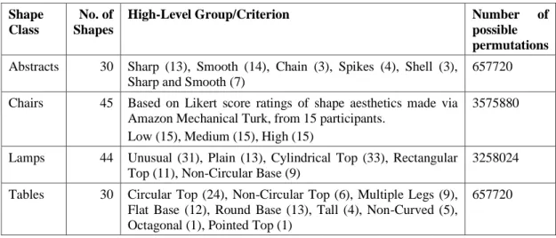
Table 2.1 – Example 2x2 contingency table ... 44 Table 2.2 – Generalised form of a 2x2 contingency table ... 45 Table 4.1 – High-level groups used to sample shapes for presentation to participants. ... 116 Table 4.2 – Summary of the collected Schelling selection data, based on high-level

groups. ... 119 Table 4.3 – Summary of the collected Schelling selection data (without high-level

groups). ... 123 Table 4.4 - Correlations between some human understandable terms (naturalness,

strangeness, and visual appeal) and Schelling frequencies (based on high-level groups). Significant correlations (p < 0.05) are in bold. ... 131 Table 4.5 - Correlations between some human understandable terms (naturalness,

strangeness, and visual appeal) and Schelling frequencies (without high-level groups). Significant correlations (p<0.05) are in bold. ... 133 Table 4.6 – k=10 fold cross-validation results from training a voxel-based neural

network for predicting Schelling saliency via 32x32x32 voxel grids (4-choose-1 approach). ... 139 Table 5.1 – Shape class sizes and the mean Schelling frequencies of each class. ... 150 Table 5.2 – Correlations between Schelling frequencies from the pots class where all 47

shapes were shown (within a larger 95 pots group) vs. Schelling frequencies obtained via showing 12 shapes at a time, incrementally... 159 Table 5.3 - Correlations between the average Likert scores for each shape (from 15

participants), and each shape’s Schelling frequencies as obtained via showing all shapes in each shape class (from 50 participants). Significant correlations (p < 0.05) are in bold... 166 Table 5.4 – Correlations between Schelling frequency predictions based on depth image

triplets and participant provided Schelling frequencies, for each shape class. .. 172 Table 5.5 – Correlations between Schelling frequency predictions and participant

provided Schelling frequencies across all shapes. ... 173 Table 5.6 - Correlations between Schelling frequency predictions based on voxel grids

and participant provided Schelling frequencies, for each shape class. Additionally, shows the correlation between the average of all sample predictions across each shape and each shape’s participant Schelling frequency. ... 174 Table 5.7 – Correlations between Schelling frequency predictions based on shape

descriptors and participant provided Schelling frequencies, for each shape class. ... 181

Table 5.8 – Adjusted Mutual Information values based on pairing a clustering derived from Schelling frequencies with a clustering based on each shape descriptor (values > 𝟐𝝈 away from the mean are in green). ... 193 Table 5.9 – Adjusted Rand Index values based on pairing a clustering derived from

Schelling frequencies with a clustering based on each shape descriptor (values > 𝟐𝝈 away from the mean are in green). ... 194 Table 5.10 – One-way ANOVA test results for significant differences in mean

memorability Likert scores of clusters obtained via k-means (k=4), across all shape classes... 198 Table 5.11 – One-way ANOVA test results for significant differences in mean ‘standing

out’ Likert scores of clusters obtained via k-means (k=4), across all shape classes. ... 199 Table 5.12 – One-way ANOVA test results for significant differences in mean

uniqueness Likert scores of clusters obtained via k-means (k=4), across all shape classes... 200 Table 5.13 – One-way ANOVA test results for significant differences in mean visual

appeal Likert scores of clusters obtained via k-means (k=4), across all shape classes... 201 Table 5.14 – One-way ANOVA test results for significant differences in mean Schelling

frequency of clusters obtained via k-means (k=4) for various shape descriptors, across all shape classes. ... 202 Table 6.1 – Statistics of the percentage of words provided only once, by participants. ... 208 Table 6.2 – Proportions of Part-Of-Speech associated with word categories. ... 212 Table 6.3 – Most frequent PoS tags of seven of the most frequent word categories. 214 Table 6.4 – Most frequent PoS tags of six of the most frequent word categories. .... 214 Table 6.5 – Correlations of Likert scores of subjective terms with Rényi Specificity

scores. Significant correlations (p < 0.05) are in bold. ... 219 Table 6.6 – Correlations between standard deviations of path similarity based font

Specificity contributions (without term-frequency weightings) and Rényi Specificity scores. ... 221 Table 6.8 – Correlations between Rényi Specificity scores, and scores obtained between

various word embeddings and formulations of font Specificity (with term-frequency weighting). Correlations in bold are significant (p<0.05)... 226 Table 6.9 – Correlations between Rényi Specificity scores, and scores obtained between

various word embeddings and formulations of font Specificity. Correlations in bold are significant (p<0.05)... 227

Table 6.11 - Correlations of Likert scores of subjective terms with word embedding-based Specificity scores. Correlations in bold are significant (p<0.05)... 232 Table 6.12 – Correlations of Likert scores of subjective terms with word embedding-based Specificity scores, given fonts with low, medium and high Specificity. Significant correlations (p < 0.05) are in bold. ... 233 Table 6.13 – Correlation between k=10 cross-validation Specificity score predictions

and actual Specificity scores of fonts (based on word embeddings), based on training examples created via font image sub-samples. ... 235 Table 6.14 – Correlations between k=10 cross-validation Specificity score predictions

and actual Specificity scores of fonts associated with training examples based on image descriptors. ... 238 Table 6.15 – Average creativity Likert scores of fonts in each row (1st=closest,

5th_{=farthest), based on 15 participants, in addition to the average score of each row} and its approximate percentile relative to the entire 100 font dataset. ... 245 Table 6.16 – Most creative (while still legible) font row selection frequencies among 30

participants. ... 245 Table 6.17 – Average legibility Likert scores of fonts in each row (1st_=closest,

5th=farthest), based on 15 participants, in addition to the average score of each row and its approximate percentile relative to the entire 100 font dataset. ... 246 Table 6.18 – Most legible font row selection frequencies among 30 participants. .... 247 Table 6.19 – Adjusted Rand Index values based on pairing k-means clusterings derived

from Specificity scores with a clustering based on each shape descriptor (values

> 𝟐𝝈 away from the mean are in green). ... 253 Table 6.20 – Adjusted Mutual Information values based on pairing k-means clusterings

derived from Specificity scores with a clustering based on each shape descriptor (values > 𝟐𝝈 away from the mean are in green). ... 253 Table 6.21 – One-way ANOVA test results for significant differences in mean

Specificity score of clusters obtained via k-means (k=4, k=8), across all 100 fonts. ... 254 Table 6.22 – One-way ANOVA test results for significant differences in mean Likert

score of clusters obtained via k-means (k=4), across all fonts. ... 256 Table 6.23 – One-way ANOVA test results for significant differences in mean Likert

score of clusters obtained via k-means (k=8), across all fonts. ... 257 Table 8.1 – Table of word groups used to analyse the collected word data. ... 315

List of Figures

Figure 1.1 – Examples of 3D shapes and 2D fonts used as part of the thesis’ Schelling

meshes and font Specificity work. ... 4

Figure 1.2 – User-chosen Schelling point distributions on polygon meshes [5]. ... 6

Figure 1.3 – Schelling mesh selections. ... 7

Figure 1.4 – Sentence-level image descriptions from Image Specificity paper [6]. Orange indicates a subject, blue indicates the action, pink indicates nouns and and red, a place. ... 8

Figure 1.5 – Word-level descriptions of fonts and associated font images. ... 8

Figure 1.6 – Example shape selections (‘4-choose-1’ approach). ... 14

Figure 1.7 – Example shape selections (‘Many-Within-Class’ approach). ... 14

Figure 1.8 – Graph-like diagram of a subset of words used to describe fonts. ... 16

Figure 2.1 – Depiction of a colour or number-based Schelling game. ... 22

Figure 2.2 – Visualisation of Histogram of Oriented Gradients as applied to an image of Lena. ... 27

Figure 2.3 – SIFT descriptor representation for a single key point ... 27

Figure 2.4 – Representation of the retinal-like sampling pattern of the FREAK descriptor ... 29

Figure 2.5 – Sobel operator applied to a picture of a landscape (original image overlaid). ... 30

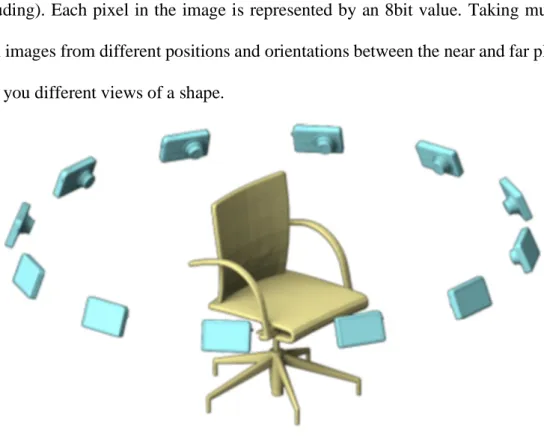
Figure 2.6 – Diagrammatic representation of depth images of a chair, taken by a virtual camera. ... 31

Figure 2.7 – Render of a polygon mesh teapot. ... 32

Figure 2.8 – Point cloud scan of a church. ... 33

Figure 2.9 – Voxelised form of the Stanford Bunny mesh. ... 34

Figure 2.10 - Diagrammatic representation of a voxel octree. ... 36

Figure 2.11 – Diagram showing principal curvature directions at a point of a hyperbolic paraboloid (saddle surface). ... 38

Figure 2.12 – Two views of a triangular polygon mesh and co-tangent angles used to compute discrete curvatures [120]. ... 38

Figure 2.14 – Example numerical Likert item ... 41

Figure 2.15 – Example text-based Likert item ... 41

Figure 2.24 – Diagram of a fully-connected artificial neural network ... 54

Figure 2.25 – Visualisation of a word vector space model, via t-SNE. ... 62

Figure 2.26 - A visual representation of the CBOW and Skip-gram vector space models, from a survey of vector-space representations of word meaning, by Camacho-Collado et al. [158] ... 62

Figure 3.1 – Image of interior surface of the eye with and with contrast enhancement. ... 67

Figure 3.2 – Diagram of the ITTI98 model [11]. ... 68

Figure 3.3 – Saliency annotation heatmaps for six image datasets (blue=low density to red=high density) [19]. ... 70

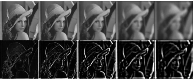
Figure 3.4 - Gaussian and Laplacian Pyramids obtained via a test image of Lena. ... 73

Figure 3.5 – Generated image variations produced via arithmetic in a latent space of image embeddings learned via a convolutional GAN [136]. (Top) Notion of ‘smiling’ is retained. (Bottom) Notion of ‘wearing glasses’ is retained. ... 90

Figure 4.1 - Shows some possible outcomes given 2, 3 or 4 options to choose from, when selecting a Schelling Point. ... 114

Figure 4.2 – Four examples of questions used to collect Schelling saliency data, one for each shape class (tables, lamps, chairs and abstract shapes). ... 118

Figure 4.3 - Four examples of “Schelling” questions (one in each row for the tables, lamps, chairs, and abstract shapes) with the participant’s selection highlighted. ... 120

Figure 4.4 – Plots of Schelling frequencies for the chairs and abstract shapes, based on high level groups ... 125

Figure 4.5 – Plots of Schelling frequencies for the lamp shapes, based on high level groups ... 126

Figure 4.6 – Plots of Schelling frequencies for the table shapes, based on high level groups ... 127

Figure 4.7 – Plots of Schelling frequencies for chair and lamp shapes, indicating how likely each shape will be selected in a Schelling sense (without high-level groups). ... 128

Figure 4.8 – Plots of Schelling frequencies for table and abstract shapes, indicating how likely each shape will be selected in a Schelling sense (without high-level groups). ... 129

Figure 4.9 – Estimated PDF of Schelling frequencies for the chairs class of shape with/without high-level groups. ... 134 Figure 4.10 – Estimated PDF of Schelling frequencies for the abstract, lamp and table

classes of shape based on high-level groups. ... 135 Figure 4.11 – Schelling saliency neural network for an input voxel resolution of

32x32x32. ... 138 Figure 4.12 - Schelling-based visualizations of chairs obtained using t-SNE. ... 140 Figure 4.13 - Schelling-based visualizations of tables obtained using t-SNE. ... 140 Figure 4.14 - Schelling-based Search. Four examples of searching with a query shape

(shown on the left). ... 142 Figure 4.15 - Schelling-based Search 2. Two examples of searching with a query shape

(shown on the left) of high Schelling frequency, one each for the chair and table shapes. ... 143 Figure 4.16 - Schelling-based Search 3. Two examples of searching with a query shape

(shown on the left) of high Schelling frequency, one each for the abstract and lamp shapes. ... 144 Figure 5.1 – Plot showing variance in Schelling frequency distributions according to

shape selections randomly sampled from 51 participants ... 156 Figure 5.2 – Visualisation of how Schelling frequencies become more stable as more

selections are gathered. ... 157 Figure 5.3 – 1-D plots of shapes at their respective participant Schelling frequencies.

We show one plot for each of the abstract shapes, tables, lamps and chairs shape classes... 160 Figure 5.4 – Plots of shape descriptor histograms for the abstracts, chairs, and tables

shape groups, with each column representing one shape, where columns are sorted according to increasing Schelling frequency. Bins with values of < 5e-3 were removed. ... 163 Figure 5.5 – Plots of shape descriptor histograms for the plants shape group, as well as

all shape groups combined, with each column representing one shape, where columns are sorted according to increasing Schelling frequency. ... 164 Figure 5.6 – A diagram showing the structure of a convolutional neural network for

predicting Schelling frequencies. ... 171 Figure 5.7 – A diagram showing the structure of a convolutional neural network for

predicting Schelling frequencies. ... 177 Figure 5.8 – Various meshes before and after the mesh processing required for

Figure 5.8 – Plots of shapes displayed in rows according to how close they are to a query shape, on the left of each plot. ... 183 Figure 5.9 - 1-D plots of shapes at their respective participant Schelling frequencies.

We show one plot for each of the pots, and cups shape groups. ... 184 Figure 5.10 - 1-D plots of shapes at their respective participant Schelling frequencies.

We show one plot for each of the abstract shapes, tables, lamps, bottles, chairs, and plates shape groups. ... 185 Figure 5.11 - Plots of the plates and tables shapes according to the 2D t-SNE embedding

of their neural network outputs from layer n-1 ... 187 Figure 5.12 - Plots of the abstracts and bottles shapes according to the 2D t-SNE

embedding of their neural network outputs from layer n-1 ... 188 Figure 5.13 – Visualised Schelling frequency based clusterings (k-means) for the

bottles, chairs and cups. ... 189 Figure 5.14 – Visualised Schelling frequency based clusterings (k-means) for the

abstract shapes and plates. ... 190 Figure 6.1 – Plots of per-font word frequency statistics across participants. ... 208 Figure 6.2 – A plot showing the proportion of words provided once for each font, across

all 111 participants. ... 209 Figure 6.3 – Word frequency plot of the top-50 most frequent words across all fonts. ... 210 Figure 6.4 – Plots of word and word group frequency, per category. ... 213 Figure 6.5 – Visualisations of Rényi Specificity... 217 Figure 6.6 – Plot showing Rényi Specificity decreasing with the frequency of unique

words associated with a font (corr.=-0.7544, p << 0.05). ... 218 Figure 6.7 – Image visualising cosine similarity between two word vectors ... 223 Figure 6.9 – (Top) Estimated PDF of word embedding-based Specificity scores and

(Bottom) their empirical CDF (blue), with a fitted curve overlaid (green). ... 229 Figure 6.10 – Plots created via word embedding-based font Specificity scores. ... 230 Figure 6.10 – Plot showing word embedding-based Specificity decreasing with the

frequency of unique words associated with a font. ... 231 Figure 6.11 – Plot of the bottom-10 and top-10 fonts according to their word

embedding-based Specificity scores. ... 232 Figure 6.12 – Diagram of a convolutional neural network for word embedding-based

font Specificity prediction. Takes as input a 200x200 sub-image of a font, and outputs a font Specificity prediction, 𝒚𝒊. ... 239

Figure 6.13 – Visualisation of 100 font t-SNE embedding based on outputs of our font Specificity prediction model. ... 241 Figure 6.14 – Rows of fonts shown to participants in font creativity and legibility

surveys for comparison of Specificity to shape descriptors. Each query font is located under each category (this was hidden from participants). ... 244 Figure 6.15 – Visualised Rényi Specificity-based clustering (k-means; k=4) for all 100

fonts. For each cluster, the mean and standard deviation of the Specificity scores of its constituent fonts is displayed. ... 249 Figure 6.16 – Visualised word2vec Specificity-based clustering (k-means; k=4) for all

100 fonts. For each cluster, the mean and standard deviation of the Specificity scores of its constituent fonts is displayed. ... 250 Figure 6.17 – Visualised SIFT-based clustering (k-means; k=4) for all 100 fonts. ... 251 Figure 6.18 – Visualised PCA-HoG-based clustering (k-means; k=4) for all 100 fonts. ... 252 Figure 8.1 - Screenshot of an Amazon Mechanical Turk hosted survey that we provided

to participants. ... 299 Figure 8.2 – Visualised D2 descriptor based clusterings (k-means) for the abstract

shapes and plates. ... 300 Figure 8.3 – Visualised D2 descriptor based clustering for the bottles and Sobel-based

clustering for the chairs (k-means). ... 301 Figure 8.4 – Visualised Sobel-based clustering for the cups (k-means). ... 302 Figure 8.5 – An example of a survey that we provided to participants. ... 303 Figure 8.6 – Example Likert survey shown to participants, for data collection of

subjective terms. ... 304 Figure 8.7 – Screenshot of survey on font creativity held via Amazon Mechanical Turk. ... 305 Figure 8.8 – All 100 fonts sorted according to word2vec-based Specificity scores (in

ascending order). ... 310 Figure 8.9 – Plots of the top-50 words’ frequencies for the bottom 2 groups of 20 fonts

sampled according to increasing word embedding-based Specificity score (without replacement) - top (font #1 to #20), bottom (font #21 to #40). ... 311 Figure 8.10 – Plots of the top-50 words’ frequencies for the mid-to-high score groups

of 20 fonts sampled according to increasing word embedding-based Specificity score (without replacement) - top (font #41 to #60), bottom (font #61 to #80). 312

Figure 8.11 – Plots of the top-50 words’ frequencies for the highest score groups of 20 fonts sampled according to increasing word embedding-based Specificity score (without replacement; font #81 to #100). ... 313

1

Introduction

Shapes in general, are used to convey meaning. 3D shapes are used in video games, films and other multimedia, in diverse ways. Fonts are the most common 2D shapes seen every day. But, understanding how users perceive and interact with shapes is a relatively new area of work. This could allow software to be more adaptable to a user’s wants or needs. Examples could include visualisation of shapes according to aspects of human perception, and prediction of shapes which most exhibit these properties. Eventually, people’s ideals could be in some way expressed in the software which they use, guiding and supporting further development of these ideas.

The field of 3D modelling focuses on the creation of tools and techniques for computer-aided design of 3D shapes. These shapes may be destined for virtual scenes, such as those of a videogame, or instead represent objects to be constructed in the real-world. 3D shapes designed for physical construction have varied complexity in their geometry. They may exude the simplicity of a ceramic bowl or reach the detailed intricacy of a sports car. Computer-generated animations use 3D shapes to produce majestic environments and the characters within them, expressing a story from the characters’ point of view. Sometimes, this can be done simply through a character’s facial

expressions and gestures, expressing their emotion as the story progresses. 3D shapes can additionally be used for data visualisation, allowing one to look at slice of a set of high-dimensional data. For a more concrete example, we can visualise tissue samples via MRI (Magnetic Resonance Imaging) scans.

Fonts can be interpreted as additional properties or transformations of a baseline alphabet, which enable different visual expressions of text. Examples include size/scale, font weight and kerning (adjustment of space between characters). Fonts are used across many written and typed works, from letters and notes, to film scripts or posters. They can indicate the structure of a document, at a glance. They add character to an otherwise plain block of text, allowing the writer to make important points more visually prominent or distinct from other text. Through computers, more varied font geometries can be expressed in webpages and typed documents created with word processing packages. These can be changed on a whim, as the user prefers. Typography is a related field of work which aims to discover techniques to style, arrange and change the appearance of text, to make it more legible and visually appealing to a reader. This can be done via modification of font sizes, kerning, character width/length, and the lengths of edges/lines within characters.

1.1

Problem Space

In general, there is a lot of data available from many different sources of multimedia, comprised of many categories. Sources include social media sites such as: Instagram,

Flickr, Facebook, and Twitter – which predominantly provide images and text. Game

asset stores associated with Unity and Unreal Engine, provide animation data, 3D shapes, textures and more. Trimble 3D Warehouse [2] could also be included under this category, for provision of 3D shapes. Audio can be freely obtained and streamed via

Soundcloud. Many wallpapers and fonts are freely available under creative commons licensing. Every day, photographs of moments in people’s lives are captured, videos are uploaded, audio tracks created, and 3D shapes modelled, adding to these vast databases of multimedia. There are many types of media and data, from many sources… But how can we organise this data? We may be able to organise it geometrically, but is this what people choose or prefer?

If we wish to organise data from a view of human perception or user preference, it becomes increasingly difficult to organise and interpret this data in a multi-modal manner, so we tried to understand at least a subset of it, in this way. We focused on 3D shapes and 2D fonts, as they are forms of geometry independent of colour, lighting and other attributes, such as colour images. Restricting ourselves in this way would help to narrow down potential variables in our studies. Figure 1.1 provides some examples of the data that we collected and used.

When people study 3D shapes and 2D fonts, they typically use traditional geometric shape descriptors. These are an approximate description of some aspect of a shape’s geometry, such as its curvature (see sections 2.1.3, 2.2.2 and 2.3.2 of the Background

chapter for more details). Curvature has been related to shape aesthetics or beauty in architecture [3]. It has been shown that when people contemplate beauty, viewing contours exclusively activates a region of the brain “strongly responsive to the reward properties and emotional salience of objects” [3].

Figure 1.1 – Examples of 3D shapes and 2D fonts used as part of the thesis’ Schelling meshes and font Specificity work.

But, are shape descriptors necessarily enough to understand how people interact with and want to organise 3D shapes and 2D fonts? People have different preferences and provide different interpretations of the same objects, but nevertheless, it has been shown that there can be some level of agreement between our perceptions of geometry [4], which we believe can be exploited for creative applications, such as product design or advertising. More generally, we may be able to use this understanding for search or visualisation applications based on perceived attributes of some geometry, with respect to other geometry of similar function. For example, a single armchair vs. other chairs, or a creative font vs a group of simpler, more legible fonts.

Some typical geometric representations of 2D images and 3D shapes are described in sections 2.2.1 and 2.3.1 of the Background chapter, respectively.

1.2

Theme

In this thesis, we introduce new ways to understand 2D fonts and 3D shapes, by measuring and discovering human-perceptual aspects of their geometry, via the concepts of Schelling Points [5, 6] and Specificity [7].

We define a human interpretation of shape as a subjective response to some visual stimuli in the form of a shape, based on the visible geometric structure and/or topology of that shape.

Our approach differs from the traditional approach of saliency detection on individual shapes or fonts, as a basis for understanding them. We instead use a data-driven

approach where we collect data based on a human interpretation of their geometry relative to other shapes and use this data to better understand them.

1.3

Methodology

Here we provide our methodology for studying and understanding 3D shapes and 2D fonts, which focuses on human perception. We use the concepts of Schelling points or Specificity as tools for this purpose.

1.3.1

Concepts

Schelling Points

An example of human interpretation that we focused on, is the notion of a Schelling

Point. Schelling Points (or focal points) are a concept invented by Thomas Schelling

[5]. They are choices that people make when they aim to match with what they expect others to choose but cannot communicate with others to determine an answer (see section 2.1.1 of the Background chapter for more details). Previous work has studied points on 3D meshes selected by people due to their salience in this coordination game

setting [6]. Participants aimed to select vertices that they believed others would also pick.

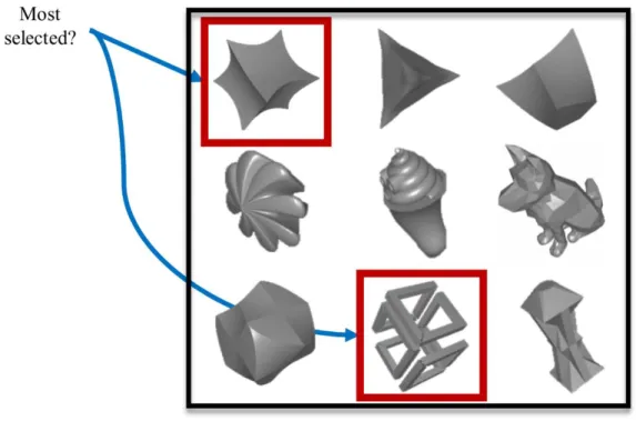
Existing work had not collected data on whole shape selections from a set of shapes, so we took this approach. When participants are given the task of matching other people’s shape selections, we name the most selected shapes under this setting, ‘Schelling meshes’ (as we intend them to be in the form of polygon meshes). These could be described as the most salient meshes within that set, given the task. Examples of Schelling point distributions on meshes are shown in Figure 1.2, in addition to examples of Schelling mesh selections in Figure 1.3, the latter of which, we collected in our work.

Figure 1.3 – Schelling mesh selections. An example of user-chosen Schelling meshes out of a class of shapes.

Specificity

Another example of human interpretation is the notion of Specificity. The origin of the term is from the Image Specificity work [7], where the authors asked people to describe images via sentences of text. Each image consisted of a scene of objects and was associated with multiple sentences.

The key idea behind Specificity is that different images evoke different descriptions, but

‘Specific’ images yield more consistent descriptions than others. These images could be

photographs, each depicting a real-world scene, as in the original Image Specificity

work, or images of individual objects with unique details (see section 2.1.2 of the

Existing work had only studied the Specificity of photographic images. Inspired by this, we focused on applying the concept of Specificity to 2D fonts. An example image description from the Image Specificity paper is provided in Figure 1.4, along with an example from the work in this thesis, in Figure 1.5.

Figure 1.4 – Sentence-level image descriptions from Image Specificity paper [7]. Orange indicates a subject, blue indicates the action, pink indicates nouns and

and red, a place.

Figure 1.5 – Word-level descriptions of fonts and associated font images.These were collected as part of the thesis’ font Specificity work.

Group-level Saliency

These two measures share some common concepts. Firstly, they require some notion of relative comparison between objects within a group. They also treat shapes as discrete objects (rather than continuous ones). Schelling Points reflect how distinctive an element of a group is, with respect to the other elements of the group. In some way, a Schelling point is a quintessential element of that group. A Specific element of a group is likely to be one which can be represented using the least amount of information, with respect to the other elements of the group. Each measure therefore depends on the distribution of the group’s objects. For example, if the group is a class of 3D shapes, the class’ distribution could be represented through many potential factors: how varied each shape’s surface geometry is; the intended function of each shape, or the familiarity of an observer with each shape’s structure. Overall, these approaches allow you to measure complementary aspects of the shapes within a group, that are different to the underlying geometry – e.g. perceived creativity, memorability.

These are Group-level saliency approaches. Unit-level saliency approaches describe or focus on an individual object at a time, with a goal of understanding which sub-components of a single object are salient. Group-level saliency involves the comparison of whole, discrete objects (a raster image; a polygon mesh) – possibly via derived information such as textual descriptions, whereas unit-level saliency uses approximations to continuous elements (pixels, polygons, voxels, superpixels etc) to describe a single object.

For a group-level saliency example, we might develop a measure of ‘distinctiveness’ for 3D shapes, which for a chair might suggest how extreme it is relative to traditional designs (armchairs, wooden chairs, stools etc.). By keeping track of this measure over time, we can see how well the individual chairs within a group can be distinguished

from the rest of the group, at regular time periods. It may be possible to make long-term predictions about the group. If we try to predict the ‘distinctiveness’ of new chairs, via a regression model, it can be treated as a population-level statistic for the chairs.

1.3.2

Research Questions

Schelling Meshes

Based on the Schelling Points concept, we tried to understand which 3D shapes are selected by people when they want to match shapes that others will pick.

The assumption was that there existed some level of agreement between the shapes that people would select, either exact (‘as-a-whole’ shape choice), or correlational (based on the properties of a subset of the shape collection shown to them), that we could exploit. Overall, we aimed to determine the degree of this agreement, across different classes of 3D shape.

Research Question: Can we understand more about the Schelling concept, in the context of 3D shapes, and apply this concept in a useful manner?

Importance: We believed this could be a basis for a group-level saliency of 3D shapes, allowing for relative comparison between shapes, via complementary subjective factors to that of the shape geometry – e.g. creativity, memorability. From this, group-level saliency predictions could then be possible for new meshes in a class, via a machine learning model based on collected data. A measure like this could be used to organise shapes using perceptual information, to attract attention to safety indicators or potential advertising.

Aims: The aim of our work was to understand 3D shapes in the specific "Schelling" context. We wanted to understand Schelling meshes by collecting data on the concept.

We aimed to characterise the notion of Schelling meshes and determine whether it could help us further understand 3D shapes, for applications in search, visualisation and/or clustering.

Potential Applications

If Schelling meshes are consistent among a class, there is likely at least one complementary aspect to those shapes which causes them to be selected. This perceived factor could for example, be a notion of creativity among the shapes. Other potential candidates may include: uniqueness, memorability, and so-on…

This knowledge could enable new methods of shape visualisation which adapt how shapes are viewed, based on some complementary aspect of their geometry. For example, less creative shapes could be given contrasting colours compared to more creative shapes, when compared in a uniform colour case (e.g. all shapes are grey).

Additionally, 3D products and packaging could be designed around automatically generated shapes which exhibit geometry considered to be most memorable, for more effective advertising.

Font Specificity

Using the concept of Specificity, we attempted to understand whether 2D fonts can be consistently described, when done in a subjective manner.

We took a similar approach to that of Image Specificity [7], in that we asked people to describe images of fonts via text, but we requested that words be provided, instead of sentences. We showed only one font per image, which lacked the scene-level complexity of images being described in the Image Specificity work. Each image consisted of a single font and was associated with multiple words. As these words each

conveyed different meanings (word senses), different words influenced the overall subjective response from participants, in different ways. Overall, ‘Specific’ fonts yielded more consistent descriptions than others – from measurement based on word frequency, or word co-occurrence probabilities (word embeddings).

Research Question: Can we understand more about the concept of Specificity, in the context of 2D fonts, and apply this concept in a useful manner?

Importance: We believed this could be a basis for a group-level saliency of 2D fonts, allowing for relative comparison between fonts, via complementary subjective factors to that of the fonts’ geometry – e.g. legibility, creativity, elegance. Given some measure of Specificity, group-level saliency predictions could then be possible for new fonts relative to the original set, via a machine learning model based on collected data. These could be used to organise fonts using perceptual information in a way that is closer to that of natural language concepts which a user of some software may intend to filter or process by. From this, we imagined that applications in search, visualisation and/or clustering could exist, and possibly other areas such as word-processing or syntax highlighting.

Aims: The aim of our work was to understand 2D fonts under the context of Specificity. We wanted to understand font Specificity by collecting data on the concept. We aimed to characterise font Specificity and determine whether it could help us further understand fonts, for applications in search and visualisation.

Potential Applications

Specific fonts are likely to be those that look the most geometrically simple, since people find fewer ways to describe them. These may be the most legible fonts, but least creative fonts. Assuming this is true, Specificity could be helpful in situations where a

user may want to select fonts which complement and contrast text, or possibly fonts which aid in memorability and clarity of text.

Search applications could for example, rank a selection of fonts according to their Specificity, with fonts high in value being used to emphasise important text within a document – and vice-versa. This could be a helpful extension to a word processing package, as it is easy to select a font and never change it – simply due to its common use, or choice as a social standard. A word processor could use this information to automatically find combinations of fonts for a title, document headings and body text, providing potential style suggestions. Additionally, in a programming development environment, we might want to automatically choose more creative fonts for syntax highlighting, relative to the main body of code.

1.3.3

Data Collection

As a basis for measuring which 3D shapes were most likely to be Schelling meshes, and fonts, most Specific, we collected data on 3D shapes and 2D fonts using the Amazon Mechanical Turk crowdsourcing platform. Shapes were shown as gif images undergoing looped 360° rotation, and fonts were shown as static png images. Cylindrical rotation was provided, as most objects people come across are placed in an upright orientation. Additionally, a single axis of rotation was used to encourage continuity in the rotation, avoiding sudden changes attracting attention. We firstly obtained a dataset of 3D polygon meshes, split into various classes (e.g. tables, chairs, lamps etc.) and additionally, a collection of greyscale fonts. We then collected shape selections made under the Schelling context, for separate classes of 3D shape, in addition to textual data for fonts. Examples are shown in Figure 1.6 and Figure 1.7. Shapes were collected from the ShapeNet dataset [8], and fonts from fontlibrary.org.

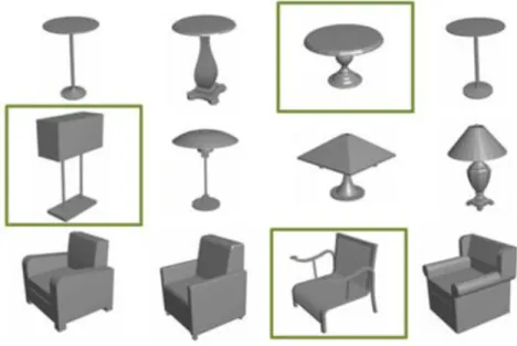
Figure 1.6 – Example shape selections (‘4-choose-1’ approach). Each row is a question, with an example answer highlighted (selected shape out of four).

No examples were shown to participants prior to completing a survey. A qualification survey was used to filter participants.

Figure 1.7 – Example shape selections (‘Many-Within-Class’ approach). An example question with example answers highlighted (4 out of 15 abstract shapes).

No examples were shown to participants prior to completing a survey.

For the ‘4-choose-1’ case, selection data consisted of one chosen shape out of four shapes. People selected each shape with the aim of matching with what they expected others to choose, given that permutation of four shapes. Group-level saliency should be

measured across an entire class, but through many permutations of four shapes being shown, relative selection frequencies can be obtained per shape, within the class. In studying these frequencies, we assumed that studying permutations of 4 shapes could lead to the discovery of class-level properties of the shapes. A simple qualification test was carried out, showing questions consisting of four shapes, where was one was unique and the other three were the same. The unique shape was required to be selected across 70% of all questions, for the participant to be allowed to complete a full survey. For the ‘Many-Within-Class’ case, selections consisted of one or more chosen shapes from a class of shapes, where people selected shapes with the aim of matching with what they expected others to choose. We reiterated this point, with a reminder before each question. We found that this was enough to achieve good results across shape classes, without a qualification test.

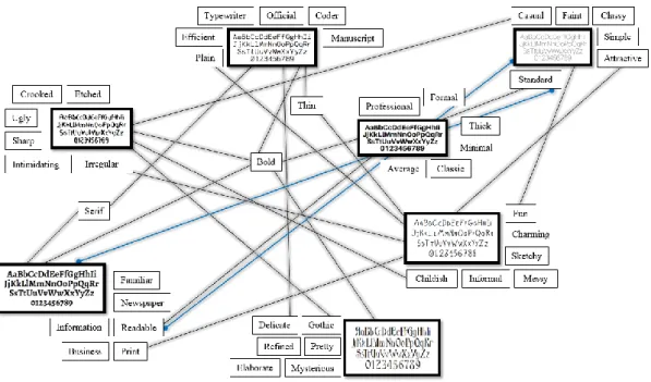
For each of the fonts, we collected human descriptions in the form of words. We focused on the consistency of the descriptions, to determine font Specificity. Due to this, we studied per-font word distributions (see sections 6.4.4 and 6.4.5). Figure 1.8 shows a selection of fonts varied in Specificity, grouped with the words used to describe them. These words were collected from people as part of the thesis’ font Specificity work. Lines in blue are ambiguous due to overlap with other elements of the diagram, so connections are shown via the terminating circles at the ends of those lines.

Figure 1.8 – Graph-like diagram of a subset of words used to describe fonts. Fonts are linked to words used to describe them, collected as part of the thesis’

font Specificity work. Words unique to each font are placed nearby the font, without any connection. Blue lines are connected at their circular end-points to

avoid ambiguity.

1.3.4

Analysis

Using the collected shape selection data, we calculated Schelling frequencies, or the frequency of a shape’s selection made under the Schelling context, given how many times it was visible (unless stated, all participants could see all shapes). We could then order the shapes according to these frequencies, allowing us to visualise them and look for initial patterns. We also held separate surveys to determine whether Schelling frequencies correlated with other subjective terms (e.g. ‘visual appeal’, ‘memorability’), and to what degree (these were determined via comments from a small initial survey). Additionally, we determined via statistical tests whether selection frequencies were consistently distributed among different groups of participants, given the same questions (see sections 4.4.4 and 5.4.1). The Background chapter summarises a range of statistical tests used throughout the thesis (see section 2.5.2).

Using the collected word-level descriptions of fonts, we computed word frequency-based Specificity scores for each font. Statistical testing was employed to check for consistency in word frequency distributions obtained from different groups of participants (see section 6.4.5). In subjective terms, we held surveys via Amazon Mechanical Turk, to determine whether Specific fonts were considered to be visually appealing, creative, or more legible etc, via Likert score ratings of individual fonts, for each of the terms. The chosen terms for the Likert surveys were sampled from the top-50 most frequent words provided by participants (see Figure 6.3), and topics/subjects associated with those words. We also produced an automated approach to compute font Specificity scores, by representing words assigned to fonts as vectors in a word embedding (see section 2.6.5 of the Background chapter for more details). Using these automated scores, we determined the properties of the most Specific fonts – for example, were they mostly bold, italic or of simple geometry? We conducted additional surveys via Amazon Mechanical Turk, to determine whether Specific fonts from a view of the automated approach, were considered to be visually appealing, creative, or more legible etc.

1.3.5

Learning

Using our collected data, we aimed to create models to predict some human-perceptual aspects of our collected 3D shape and 2D font datasets, based on the concepts of Schelling meshes and font Specificity.

To predict Schelling meshes and Specific fonts, we predominately used convolutional neural networks. Regarding Schelling meshes, we created two approaches: 1) a voxel-based convolutional neural network which predicts the relative selection probability of a shape given three other shapes in its class, and 2) a depth image-based convolutional

neural network which predicts a shape’s Schelling frequency relative to its class of shape, given a triplet of orthogonal depth images each representing a shape. Data augmentation was employed by sampling different triplets from different initial positions around a shape (via rotations). In comparison to the latter approach, we also tested if geometric descriptions of 3D shapes (represented as individual vectors, or more precisely, histograms over per-vertex shape descriptor values), could be used to predict Schelling frequencies, using a fully-connected neural network. We additionally tested a voxel-based convolutional neural network for Schelling frequency prediction.

Regarding 2D fonts, we created a depth image-based convolutional neural network to predict how Specific a font is. As input, it takes an image representation of a font, mapping it to a single Specificity score, expressing the consistency of words associated with that font. We also tested if geometric descriptions of fonts (represented as individual vectors), could be used to predict font Specificity scores, using a fully-connected neural network.

1.4

Thesis Organisation

1.4.1

Layout and Structure

Following the Introduction is a Background chapter, covering key concepts needed to understand the work in this thesis, such as information on geometry representations, data collection, statistical tests / analysis, and relevant topics in machine learning.

Afterwards is the Related Work chapter, which provides an overview of previous research that is related to the theme of the thesis. It covers four main topics: 1) Saliency + Shape Perception, 2) Understanding of Geometry, 3) Machine Learning, and 4) Crowdsourcing. A summary is provided for each topic. In the conclusion section of the

chapter, research gaps are indicated which are most relevant to the thesis research, highlighting the contributions we provide that complement the existing literature.

In the Schelling Meshes: ‘4-choose-1’ chapter, we introduce the notion of ‘Schelling meshes’, an approach to understanding 3D shapes via a basis of human preference. We study the agreement between participants when they select one out of four shapes, aiming to match other people’s selections. We detail our data collection method, interpret and analyse the results, and describe our approach to learning and predicting which shape is most likely to be a Schelling mesh out of a group of four shapes. We also provide potential applications in search and visualisation, using shape selection frequencies given shape visibility by participants. To conclude the chapter, we discuss the approach and report our main findings.

The next chapter (Schelling Meshes: ‘Many-Within-Class’) introduces an approach to collecting data on Schelling meshes where participants can select multiple shapes within a class, aiming to match others’ selections, as before. We interpret and analyse our results and provide a method to predict how likely a shape is to be a Schelling mesh out of a shape class. This is our ‘Many-Within-Class’ approach. To conclude the chapter, we report and discuss our main findings.

To follow, we study 2D shapes in the Font Specificity chapter. This covers our approach to understanding 2D fonts via the concept of Specificity. We detail our data collection approach and show the results of our analysis. Based on these results, we show how per-font word distributions can be used to create a Specificity score and detail an approach to automatically compute Specificity scores with similar properties. We also provide a method to predict font Specificity and introduce potential applications in

search, visualisation and clustering. To conclude, we report and discuss our main findings.

We end the thesis with a Conclusions chapter, discussing how the topics of Schelling meshes and font Specificityrelate to the thesis’ theme of understanding 3D shapes and 2D fonts via human-perceptual aspects of their geometry. We provide potential future applications, and areas of research that could follow from this work.

1.5

List of Main Contributions

• Data Collection: Via crowdsourcing, we study what makes a shape more Schelling than others, and a font more Specific than others.

• Analysis: We create a scoring approach for meshes, by treating them as Schelling points, and create measures of Specificity for fonts. We determine subjective properties common to Schelling meshes or Specific fonts.

• Learning: We show that a function to predict which shapes are likely to be Schelling meshes can be learned for different classes of shape. Such a learned function can then be used to make predictions for any new shape, within the same class. We also show that Specificity can be learned for fonts, which similarly can be used to predict Specificity for any new font.

• Applications: We show that 3D shape or 2D font datasets can be clustered or directly visualised using the concept of Schelling meshes, or Specificity for fonts. This data can also be used to search for the most legible fonts, or shapes that stand out most, in a collection.

2

Background

2.1

Concepts

2.1.1

Schelling Points

Schelling Points are those choices people make when they aim to maximise their

payoff/reward in a hypothetical game but cannot communicate with others to determine an answer – in other words, they may have imperfect information. When the goal of this game is to “be in agreement with others, as much as possible” (an example of a co-ordination game), they are choices selected by people when they choose to match each other’s selections, with no communication beforehand [5]. For example, if two people are driving down a single path, one car travelling down from either end, but they wish to avoid a collision, they need to choose a convention to avoid that collision. If there is enough space to overtake each other’s car, they might both signal to only turn left, or only turn right, keeping themselves safe. Without the necessary space, they would likely slow their car down as soon as possible! The Schelling points are either to press the brake or turn in the same direction.

We can take colour selection as another example (see Figure 2.1). When people are asked to select from four colours, three of which are blue and one, red, they are more likely to select red. Given four numbers, three of which are ‘1’ and one, ‘3’, they are more likely to select ‘3’. In the former case, there is some psychological basis or consistency behind the selection of the red colour. In the latter case, the relative change in the geometry of the fonts representing each number is the stimuli behind the selection of the number ‘3’. This implies that studying these selections can help to study some

aspect of human visual perception, as a top-down approach. Humans are adept at detecting patterns in a visual scene, due to the accuracy and speed of the human visual system (HVS), so aspects of these patterns should contribute to their selection decisions.

Figure 2.1 – Depiction of a colour or number-based Schelling game.

Works which involve Schelling Points aim to define some unit of selection, which in the most abstract sense is of a collection of objects. A special case of this could be a class of 3D shapes. From these, we may want to refine the selection unit down to a single shape, a region of a shape, or its base elements, such as vertices or voxels (which would be analogous to pixels in 2D images).

Previous work has studied points on 3D meshes selected by people due to their salience in this coordination game setting [6]. Participants of a crowdsourced survey aimed to select vertices on a mesh that they believed others would also pick. These could then be treated as Schelling points. Using the obtained data, a regression model was learned to predict where Schelling points would mostly likely be on a new mesh.

2.1.2

Specificity

Specificity stems from the consistency of descriptions associated with an object [7]. These descriptions might be phrases or sentences made up of unit words, or textural or colour-based symbols representing concepts of the object. If we ask people to describe an object, we expect can varied precision, from precise mathematical definitions or

statements to subjective terminology. But, since people want interpretability with little cost, they describe objects with some accuracy in-between this spectrum. Therefore, humans informally communicate via some natural language, where there is agreement on how to represent common concepts via words and punctuation, structured via a set of grammar rules.

Determining the Specificity of an object requires a set of words which are descriptive of the object, where each word is compared relative to one another within the set. Some value is obtained for each comparison, which for example, might be some occurrence frequency or ratio of occurrence frequencies, but overall it represents how common each element is, with respect to the others in the set. The average or a weighted average of these values results in a measure of Specificity for the object.

The origin of the term ‘Specificity’ comes from the Image Specificity work [7], where the authors asked people to describe images via sentences of text. Each image consisted of a scene of objects and was associated with multiple sentences. The key idea behind Specificity is that different images evoke different descriptions, but ‘Specific’ images yield more consistent descriptions than others. These images could be photographs, each depicting a real-world scene, as in the original Image Specificity work (see Figure 1.4, in the Introduction chapter, for examples), or images of individual objects with unique details.

The authors introduced two methods for measuring Specificity. One was based on human judgements, where participants rated the similarity of pairs of sentences without being shown the source image. Each sentence corresponded to the same source image. Participants therefore made ratings only on the textual content of each sentence.

The second method was an automated measure of Specificity based on the comparison of word synonyms between pairs of sentences used to describe an image. The similarities between word synsets (sets of word synonyms of the same meaning) between sentence pairs, contributed to the final Specificity score for an image.

The authors created a model to predict image Specificity scores, using ground-truth pairs of sentences from humans in the form of ‘positive’ examples, where both sentences came from the same source image. Pairs which were ‘negative’, did not come from the same image. The parameters of this prediction model were used to generate Specificity predictions for images not seen in their image database.

2.1.3

Shape Descriptors

Shape descriptors are designed to represent a shape’s useful information, reducing the amount of space used to represent its geometry, for a specific task. This can help minimise the amount of computation required to compare or analyse shapes.

For example, we can measure the curvature of the edges/contours of objects in an image, or intensity/colour gradients across an image or texture. Specific to a 3D shape, the distribution of face normals across a polygon mesh can be obtained, or the distances between random pairs of points on a shape’s surface, given by the D2 Distribution [9, 10].

Shape descriptors are designed to represent at least one property of a shape well, in a geometric or topological sense. This could be scale-invariance, where the values of the descriptor are unaffected by the source shape’s size in each dimension. Other properties include translation-invariance, rotation-invariance, or sometimes, invariance to different types of symmetry: extrinsic (dependent on the units/co-ordinate system to

measure the shape; has invariance under rigid transformations) or intrinsic (inherent to the shape, regardless of co-ordinate system).

We assume that the resolution of the shape’s representation that is processed (e.g. a polygon mesh), is high enough to consistently obtain properties of the shape which are close to what an ideal (usually continuous) representation would provide.

Comparison of shape descriptors usually involves a notion of distance, and so in many cases, each descriptor will be a vector of elements. These vectors can be compared using some linear algebraic distance measure, such as Euclidean Distance. Another candidate could be Mahalanobis Distance, if some notion of probability is involved in the creation of the shape descriptor, and you may want to compare the variance between its elements. A distance measure allows one to measure the (dis-)similarity of shapes, through their descriptors.

Shape descriptors are commonly used for further high-level applications, such as classification. In summary, across all shape representations, many methods of shape comparison involve the use of shape descriptors.

2.2

Understanding 2D Geometry

2.2.1

Typical Representations

2D Images

A 2D image is a contiguous structure of regions placed along two dimensions, known

as pixels, which are each assigned values. If we index into the image using integer

locations, we call the image discrete. But, if we use real-valued locations, we call the image continuous, as any index into the image is valid that lies within (and includes) the intervals used to define its boundary (width and height).

Scalar images

Pixels in scalar images are assigned a single value. For an intensity image, this indicates brightness at the pixel. A depth image is another example, where single depth value is assigned to each pixel.

Colour Images (RGB)

Instead of a single intensity/brightness value per pixel, we now associate three primary colour values (e.g. red, green and blue) with each pixel, which can be combined or interpolated via barycentric co-ordinates, to produce many different colours.

2.2.2

2D Shape Descriptors

Many shape descriptors exist for 2D shapes. We discuss relevant ones here.

Histogram of Oriented Gradients (HoG)

These are histograms which represent frequencies of gradient orientation across local regions of a 2D image. Images are split into smaller ‘cells’, by which each pixel votes/contributes its gradient direction (change in angle from a fixed initial direction vector), weighted by its magnitude [11]. Pixels in 2D are analogous to voxels in 3D, so the approach can similarly be applied to 3D shapes, after voxelisation. HoG is designed to describe variation throughout an image for example, in terms of intensity/colour change of a 2D image, or surface variation in a 3D voxel grid.

Since gradients have influence in each dimension/axis, we obtain a histogram for each axis. For an image, the resulting descriptor has two histogram dimensions and can be represented via 2D vectors, based on an ideal 2D gradient vector at each image pixel. Similarly, 3D shapes have 3D gradients, leading to a 3D histogram. In both cases, these can be treated as a single vector, via consistently ordered concatenation. See Figure 2.2 for a visualisation based on an image.

Figure 2.2 – Visualisation of Histogram of Oriented Gradients as applied to an image of Lena. (Left) Test image (Right) Dominant gradient orientations of cells

throughout the image [12, 11]. Contour Curvatures

Taking the contour curves around objects in an image (indicating change in intensity/colour, analogous to level sets of a geographical map), the curvature of each contour can be computed via derivatives at each point on each contour. This can possibly be done via a forward-backward difference calculation of the derivative, as a discrete approach.

SIFT

SIFT is an algorithm to detect key points within an image at different scales, via a Difference of Gaussian approach [13, 14]. See Figure 2.3 for a visual representation.

At each scale/octave, images are blurred at two different values of 𝜎. Across each of these blurred images, local extrema (pixel locations 0 of gradient) are searched for. SIFT scales down the image further and uses larger Gaussian kernels, at each octave. These are potential key points, which are filtered according to an intensity threshold, to remove edges. For each key point, a SIFT descriptor is produced b