ENSEMBLE-BASED SUPERVISED LEARNING
FOR PREDICTING DIABETES ONSET
N
ONSO
A
LEXANDA
N
NAMOKO
BEng (hons), MSc, AHEA
A thesis submitted in partial fulfilment of the requirements of
Liverpool John Moores University for the Degree of Doctor of
Philosophy
1 | P a g e
A
CKNOWLEDGEMENTThis thesis represents not only my work at the keyboard, but also a milestone in over three years of research work and career development at Liverpool John Moores University (LJMU); particularly within the Centre for Health and Social Care Informatics (CHaSCI). My experience at CHaSCI has been nothing short of amazing. From my first day of PhD research, I have felt at home. I have been given unique opportunities to improve my knowledge which includes engaging in teaching and learning activities, contributing in other research projects within CHaSCI, writing and presenting research papers to internal and external audience and many more. Throughout my years within CHaSCI, I have learned that there would be no research work without funding. In fact this research work is a result of funding from both LJMU and the Royal Liverpool and Broadgreen University Hospital (NHS) Trust (RLBUHT). This thesis is also the result of work and many experiences I have encountered from a lot of remarkable individuals who I wish to thank.
First and foremost I wish to thank God for granting me the strength, ability and determination to complete this PhD research. I would like to express my deepest gratitude to my family for the support they provided me through my entire life and in particular, I must acknowledge my children Leona and Logan, for putting a smile on my face each day; and my wife and best friend, Chioma, without whose love, encouragement and editing assistance, I would not have finished this thesis.
Very special thanks go out to my former director of studies, Dr Farath Arshad who retired unfortunately before my PhD ended. Without Farath’s support, I would not have had the opportunity to undertake this PhD research work. Farath believed in me from the start and that belief made a difference in my life. It wasn’t until I met her, that I truly developed an interest in Healthcare Informatics and her advice led to the work undertaken in my PhD work. She provided me with direction, technical support and became more of a mentor and friend, than a supervisor. She has been supportive since the first day we met when I helped her with a web development project. I remember she used to
2 | P a g e say something like "there would be plenty of time to relax later!" to encourage me to work harder. Farath has also supported me emotionally through the rough road to finish this thesis. During the most difficult times when writing this thesis, she gave me the moral support and the freedom I needed to carry on. I doubt that I will ever be able to convey my appreciation fully, but I owe her my eternal gratitude.
I would also like to express my gratitude to my new director of studies, Dr Abir Hussain, for her patient guidance, enthusiastic encouragement and useful critiques of this research work. Dr Abir has helped immensely to keep my progress on schedule.
Special thanks go to the other members of my supervisory team, Dr David England and Professor Jiten Vora for the assistance they provided at all levels of the research project. I benefited immensely from David’s vast knowledge and skill especially in technical writing which has helped in shaping my writing skills. Jiten provided the much needed clinical guidance but also his professional network led to the materials (data) used in this research.
I must also acknowledge Joe Bugler of Abbott Diabetes UK for facilitating the provision of data through his office to help this research work. Appreciation also goes out to Lucy Wilson for providing data at the initial stage of the research and to Danny Murphy, for his programming assistance to develop a prototype system for conference display. Many thanks to the technical support group at the School of Computing and Mathematical Science (CMS), LJMU for all of their computer and technical assistance throughout my PhD; and to the office staff Tricia Waterson, Carol Oliver and Lucy Tweedle for all the instances in which their assistance helped me along the way. Thanks also goes out to those who provided me with advice at times of critical need; Professor Abdenor El Rhalibi, Dr. William Hurst, Dr. Shamaila Iram and Dr Ibrahim Idowu. I would also like to thank my fellow PhD students at CMS, LJMU for our technical debates, exchanges of knowledge, skills, and venting of frustration during my PhD program, which helped enrich the experience.
3 | P a g e In conclusion, I recognize that this research would not have been possible without the financial assistance of the Faculty of Technology and Environment, LJMU and the IT Innovations department at RLBUHT. I also express my gratitude to the following organisations for providing travel grants for conferences: PGR, LJMU and AISB.
4 | P a g e
A
BSTRACTThe research presented in this thesis aims to address the issue of undiagnosed diabetes cases. The current state of knowledge is that one in seventy people in the United Kingdom are living with undiagnosed diabetes, and only one in a hundred people could identify the main signs of diabetes. Some of the tools available for predicting diabetes are either too simplistic and/or rely on superficial data for inference. On the positive side, the National Health Service (NHS) are improving data recording in this domain by offering health check to adults aged 40 - 70. Data from such programme could be utilised to mitigate the issue of superficial data; but also help to develop a predictive tool that facilitates a change from the current reactive care, onto one that is proactive. This thesis presents a tool based on a machine learning ensemble for predicting diabetes onset. Ensembles often perform better than a single classifier, and accuracy and diversity have been highlighted as the two vital requirements for constructing good ensemble classifiers. Experiments in this thesis explore the relationship between diversity from heterogeneous ensemble classifiers and the accuracy of predictions through feature subset selection in order to predict diabetes onset. Data from a national health check programme (similar to NHS health check) was used. The aim is to predict diabetes onset better than other similar studies within the literature.
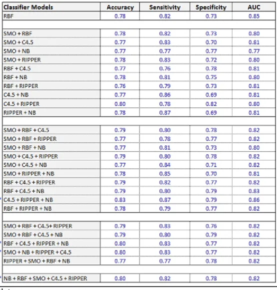
For the experiments, predictions from five base classifiers (Sequential Minimal Optimisation (SMO), Radial Basis Function (RBF), Naïve Bayes (NB), Repeated Incremental Pruning to Produce Error Reduction (RIPPER) and C4.5 decision tree), performing the same task, are exploited in all possible combinations to construct 26 ensemble models. The training data feature space was searched to select the best feature subset for each classifier. Selected subsets are used to train the classifiers and their predictions are combined using k-Nearest Neighbours algorithm as meta-classifier.
Results are analysed using four performance metrics (accuracy, sensitivity, specificity and AUC) to determine (i) if ensembles always perform better than single classifier; and (ii) the impact of diversity (from heterogeneous
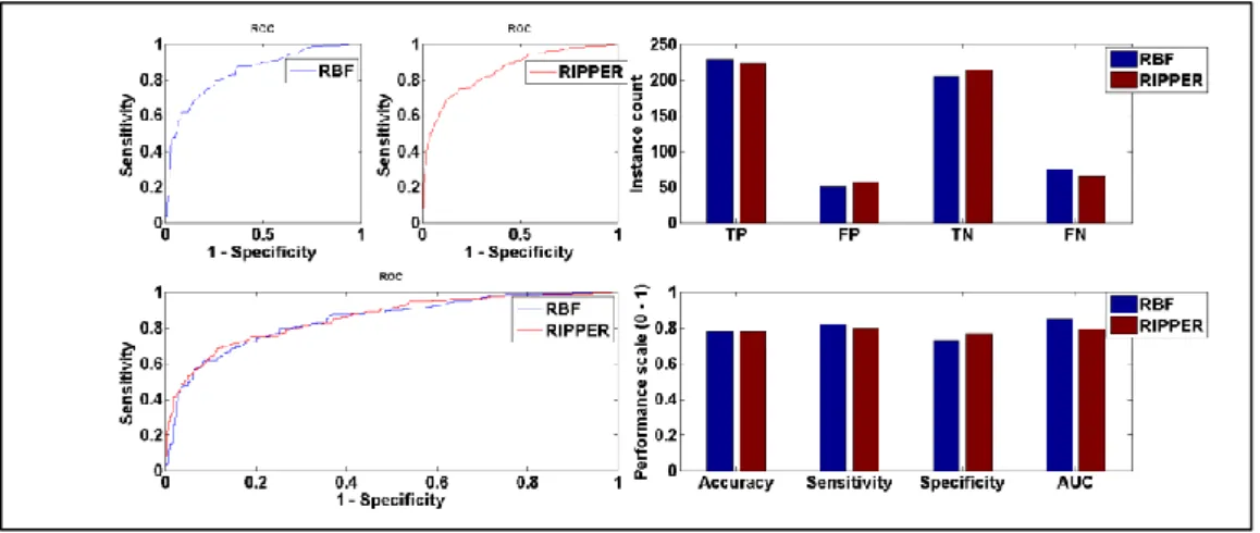
5 | P a g e classifiers) and accuracy (through feature subset selection) on ensemble performance. At base classification level, RBF produced better results than the other four classifiers with 78%accuracy, 82% sensitivity, 73% specificity and 85% AUC. A comparative study shows that RBF model is more accurate than 9 ensembles, more sensitive than 13 ensembles, more specific than 9 ensembles; and produced better AUC than 25 ensembles. This means that ensembles do not always perform better than its constituent classifiers. Of those ensembles that performed better than RBF, the combination of C4.5, RIPPER and NB produced the highest results with 83% accuracy, 87% sensitivity, 79% specificity, and 86% AUC. When compared to the RBF model, the result shows 5.37% accuracy improvement which is significant (p = 0.0332).
The experiments show how data from medical health examination can be utilised to address the issue of undiagnosed cases of diabetes. Models constructed with such data would facilitate the much desired shift from preventive to proactive care for individuals at high risk of diabetes. From the machine learning view point, it was established that ensembles constructed based on diverse and accurate base learners, have the potential to produce significant improvement in accuracy, compared to its individual constituent classifiers. In addition, the ensemble presented in this thesis is at least 1% and at most 23% more accurate than similar research studies found within the literature. This validates the superiority of the method implemented.
6 | P a g e
P
UBLICATIONSJOURNAL PAPERS &BOOK CHAPTERS:
J. Wilson, F. Arshad, N. Nnamoko, A. Whiteman, J. Ring and R. Bibhas (2013) “Patient Reported Outcome Measures PROMs 2.0: an On-Line System Empowering Patient Choice”; Journal of the American Medical Informatics Association, Vol 21, 725-729. DOI:10.1136/amiajnl-2012-001183
F.Arshad, N. Nnamoko, J. Wilson, R. Bibhas and M. Taylor (2014) “Improving Healthcare System Usability without real users: a semi-parallel design approach”; International Journal of Healthcare Information Systems and Informatics, Vol. 10, Iss. 1, 67 – 81. DOI: 10.4018/IJHISI.2015010104
N. Nnamoko, F. Arshad, L. Hammond, S. McPartland and P. Patterson (2016) "Telehealth in Primary Health Care: Analysis of Liverpool NHS Experience"; Applied Computing in Medicine and Health, Elsevier Edited Book, 269 - 286 N. Nnamoko, F. Arshad, D. England, J. Vora and J. Norman (2015) “Fuzzy Inference Model for Diabetes Management: a tool for regimen alterations”; Journal of Computer Sciences and Applications, Vol. 3, Iss. 3A, 40 – 45. doi: 10.12691/jcsa-3-3A-5
F.Arshad, L. Brook, B. Pizer, A. Mercer, B. Carter and N. Nnamoko (2017) “Innovations from Games Technology for Enhancing Communication among Children receiving End-of-Life Care”; British Medical Journal (working paper).
N. Nnamoko, F. Arshad, D. England, J. Vora and J. Norman (2017) “Ensemble Learning for Diabetes Onset Prediction”; IET Systems Biology – Special issue on Computational Models & Methods in Systems Biology & Medicine (working paper)
CONFERENCE PAPERS:
N. Nnamoko, F. Arshad, D. England, and J. Vora. (2013) “Fuzzy Expert System for Type 2 Diabetes Mellitus (T2DM) Management using Dual Inference Mechanism,” Proc. AAAI Spring Symposium on Data-driven wellness: From Self tracking to Behaviour modification, 2013
N. Nnamoko, F. Arshad, D. England, J. Vora and J. Norman. (2014) “Evaluation of Filter and Wrapper Methods for Feature Selection in Supervised Machine Learning”, 15th Annual Postgraduate Symposium on the Convergence of Telecommunications, Networking and Broadcasting, June 2014
N. Nnamoko, F. Arshad, D. England, J. Vora and J. Norman. (2014) “Meta-classification Model for Diabetes onset forecast: a proof of concept”; Proceedings of the IEEE International Conference on Bioinformatics and
7 | P a g e Biomedicine, November 2014 [Note: selected for publication in extended form in a Special Issue of the journal ‘IET Systems Biology’].
ABSTRACTS/POSTERS:
N. Nnamoko, F. Arshad, D. England, J. Vora and J. Norman (2013) “Intelligent Self-care System for Diabetes Support &Management”; Journal of Diabetes Science and Technology, March 2013.
Nonso Nnamoko, Farath Arshad, David England, Professor Jiten Vora (2015) “Evaluation of a Fuzzy Inference Model for continuous regimen alterations in Type 2 Diabetes”, Diabetes UK Professional Conference 2015
MAGAZINE ARTICLE:
Nonso Nnamoko (2014) “Social Media: an informal data source for healthcare intervention”; AISB Quarterly Magazine, 138: 20 – 22.
8 | P a g e
A
BBREVIATIONSANN: Artificial Neural Network
AUC: Area Under the Receiver Operating Characteristic Curve BG: Blood Glucose
BMI: Body Mass Index CBR: Case Based Reasoning
CHaSCI: Centre for Health and Social Care Informatics FN: False Negative
FP: False Positive FPR: False Positive Rate
HBA1c or A1c: Glycated Haemoglobin IT: Information Technology
LJMU: Liverpool John Moores University MBR: Model Based Reasoning
ML: Machine Learning NB: Naïve Bayes
NHS: National Health Service OGTT: oral glucose tolerance test RBF: Radial Basis Function RBR: Rule Based Reasoning REP: Reduced Error Pruning
9 | P a g e RLBUHT: Royal Liverpool and Broadgreen University Hospital (NHS) Trust ROC: Receiver Operating Characteristic Curve
SMO: Sequential Minimal Optimisation
SMOTE: Synthetic Minority Over-Sampling Technique SVM: Support Vector Machine
TN: True Negative TP: True Positive TPR: True Positive Rate UK: United Kingdom
10 | P a g e
T
ABLE OFC
ONTENTS Acknowledgement ... 1 Abstract ... 4 Publications ... 6 Abbreviations ... 8 Introduction ... 17 1.1 Introduction 17 1.2 Research Aims 20 1.3 Research Objectives 20 1.4 Outline of the Chapters 20 Literature Survey ... 222.1 Introduction 22 2.2 Diabetes and Screening Process 22 2.3 Computer Technology and Healthcare 25 2.3.1 Data driven Approaches To Diabetes Care 26 2.3.2 Machine Learning Ensembles 27 2.3.3 Review of Ensemble Methods and Related Research 31 2.4 Summary 38 Technical Design Components ... 40
3.1 Introduction 40
3.2 Ensemble Member Classifiers 40
3.2.1 Support Vector Machines (SVM) 41
3.2.2 Artificial Neural Network (ANN) 42
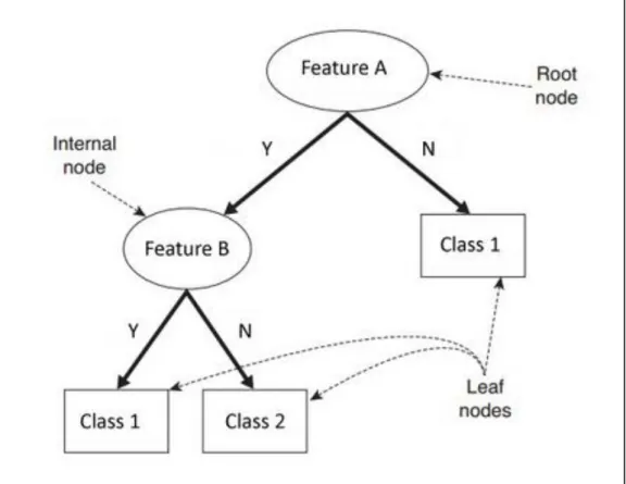
3.2.3 Decision (classification) Trees 43
3.2.4 Naïve Bayes 45
11 | P a g e
3.3 Experimental Data 47
3.4 Classifier Training Method 50
3.5 Performance Evaluation 52
3.6 Summary 55
Methodology... 56
4.1 Introduction 56
4.2 Design and Implementation 56
4.2.1 Feature Selection Approach 59
4.2.2 Stacked Generalisation 66
4.3 Summary 67
Results & Analysis ... 69
5.1 Introduction 69
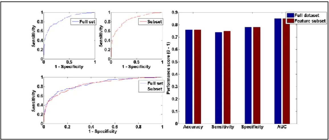
5.2 Base Level Performance with Full Training set 69 5.3 Feature selected subsets and performance 73 5.3.1 Naïve Bayes performance comparison 77
5.3.2 RBF performance comparison 78
5.3.3 SMO performance comparison 79
5.3.4 C4.5 performance comparison 80
5.3.5 RIPPER performance comparison 81
5.4 Ensemble Level Performances 83
5.4.1 Ensemble Vs Base Learner Performance 84 5.4.2 Impact of the Ensemble Method Implemented 86
5.5 Summary 92
Conclusions & Future Work ... 94
6.1 Introduction 94
6.2 Restatement of Research Purpose 94
12 | P a g e
6.4 Future Research 95
6.4.1 Variations of SMOTE Algorithm 96
6.4.2 Extended Research with different Weighted Vote 97 6.4.3 Base learner Optimisation and Further Experiments with External Dataset 99
6.4.4 Extended Research in Feature Search and Selection 100
6.5 Thesis Summary 100 Bibliography ... 103 Appendix A.1 ... 118 Appendix A.2 ... 120 Appendix A.3 ... 122 Appendix A.4 ... 126
13 | P a g e
L
ISTOFF
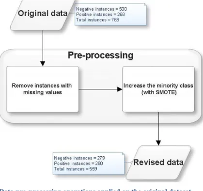
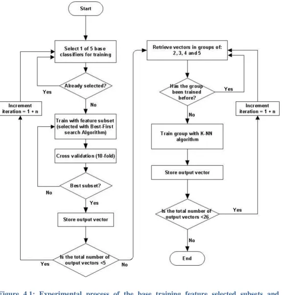
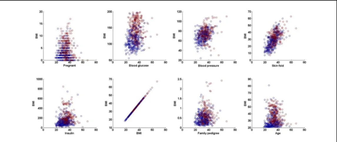
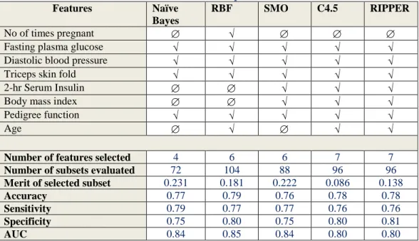
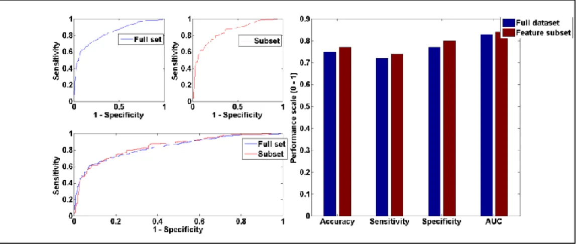
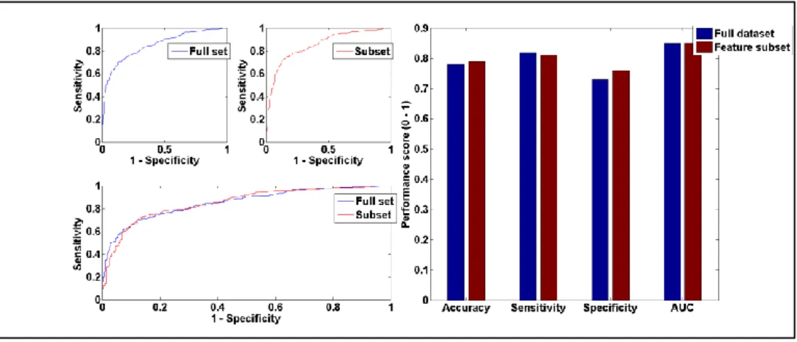
IGURESFigure 2.1: A guide for diabetes confirmatory test using HbA1c, FPG and/or OGTT (Source: [60]) ... 25 Figure 2.2: Statistical reason why good ensemble is possible (Source [28]) ... 29 Figure 2.3: Computational reason why good ensemble is possible (Source [28]) ... 30 Figure 2.4: Representational reason why good ensemble is possible (Source [28]) ... 30 Figure 3.1: Simple Decision tree structure showing the root, internal and leaf nodes. ... 44 Figure 3.2: RIPPER algorithm (adapted from [142]) ... 47 Figure 3.3: Data pre-processing operations applied on the original dataset ... 49 Figure 3.4: Visual representation of 10-fold cross validation method (Source: [154]) ... 51 Figure 3.5: Simple confusion matrix or contingency table... 53 Figure 3.6: Common performance metrics derived from a confusion matrix (Source: [157], [159]). ... 54 Figure 4.1: Experimental process of the base training feature selected subsets and ensemble training with K-NN algorithm. ... 57 Figure 4.2: Detailed diagram of feature selection (with Best-First search) and 10-fold cross validation ... 59 Figure 4.3: Best-First Algorithm with greedy step-wise and backtracking facility ... 62 Figure 4.4: A generic template for forward search (Source: [169]) ... 63 Figure 4.5: Illustration of forward and backward selection drawbacks with 3 features ... 64 Figure 4.6: A generic template for bi-directional search (Source: [169]) ... 65 Figure 4.7: Stacked generalisation using five base learners ... 66 Figure 5.1: Scatter plot showing class separation and distribution between BMI and other features of the experimental dataset. ... 70 Figure 5.2: Performance comparison between RBF and RIPPER models trained on full dataset ... 72 Figure 5.3: Naïve Bayes performance with full training set vs selected feature subset using Accuracy, Sensitivity, Specificity, AUC and Mc Nemar’s test. .. 77
14 | P a g e Figure 5.4: Graphic representation of Naïve Bayes performance trained on full dataset vs feature subset... 78 Figure 5.5: RBF performance with full training set vs selected feature subset using Accuracy, Sensitivity, Specificity, AUC and Mc Nemar’s test. ... 78 Figure 5.6: Graphic representation of RBF performance trained on full dataset vs feature subset ... 79 Figure 5.7: SMO performance with full training set vs selected feature subset using Accuracy, Sensitivity, Specificity, AUC and Mc Nemar’s test ... 79 Figure 5.8: Graphic representation of SMO performance trained on full dataset vs feature subset ... 80 Figure 5.9: C4.5 performance with full training set vs selected feature subset using Accuracy, Sensitivity, Specificity, AUC and Mc Nemar’s test ... 81 Figure 5.10: Graphic representation of C4.5 performance on full dataset vs feature subset ... 81 Figure 5.11: RIPPER performance with full training set vs selected feature subset using Accuracy, Sensitivity, Specificity, AUC and Mc Nemar’s test ... 82 Figure 5.12: Graphic representation of RIPPER performance on full dataset vs feature subset ... 83 Figure 5.13: Direct comparison of the 26 ensembles and RBF performance based on accuracy, sensitivity, specificity and AUC. ... 85 Figure 5.14: EN-mod1 vs RBF performance using Accuracy, Sensitivity, Specificity, AUC and Mc Nemar’s test ... 87 Figure 5.15: Graphic representation of EN-mod1 vs RBF model performance87 Figure 5.16: EN-mod2 vs RBF performance using Accuracy, Sensitivity, Specificity, AUC and Mc Nemar’s test ... 88 Figure 5.17: Graphic representation of EN-mod2 vs RBF model performance on AUC. ... 89 Figure 5.18: EN-mod1 vs EN-mod3 performance using Accuracy, Sensitivity, Specificity, AUC and Mc Nemar’s test ... 91 Figure 5.19: Graphic representation of EN-mod1 vs EN-mod3 model performance on AUC. ... 91 Figure A.2.0.1: SMOTE algorithm (source: [151]) ... 120 Figure A.3.0.1: Graphic representation of Naïve Bayes performance on balanced vs unbalanced dataset ... 122 Figure A.3.0.2: Graphic representation of RBF performance on balanced vs unbalanced dataset ... 123
15 | P a g e Figure A.3.0.3: Graphic representation of SMO performance on balanced vs unbalanced dataset ... 124 Figure A.3.0.4: Graphic representation of c4.5 performance on balanced vs unbalanced dataset ... 124 Figure A.3.0.5: Graphic representation of RIPPER performance on balanced vs unbalanced dataset ... 125 Figure A.4.0.1: Data cluster of ‘age’ and other features of the training dataset ... 126 Figure A.4.0.2: Data cluster of ‘family pedigree’ and other features of the training dataset ... 126 Figure A.4.0.3: Data cluster of ‘bmi’ and other features of the training dataset ... 126 Figure A.4.0.4: Data cluster of ‘insulin’ and other features of the training dataset ... 127 Figure A.4.0.5: Data cluster of ‘skin fold’ and other features of the training dataset ... 127 Figure A.4.0.6: Data cluster of ‘blood pressure’ and other features of the training dataset ... 127 Figure A.4.0.7: Data cluster of ‘blood glucose’ and other features of the training dataset ... 128 Figure A.4.0.8: Data cluster of ‘pregnant’ and other features of the training dataset ... 128 Figure A.4.0.9: Scatter plot of the experimental dataset showing class distribution and density... 128
16 | P a g e
L
ISTOFT
ABLESTable 2.1: Guidelines for Body Mass Index classification and associated diabetes risk (Source [59]) ... 24 Table 3.1: Five broad machine learning approaches and associated algorithms considered in this chapter. ... 41 Table 3.2: Characteristics of the Pima diabetes dataset from UCI database .... 48 Table 3.3: Characteristics of the revised dataset obtained from the Pima diabetes data... 50 Table 3.4: Comparing k-fold cross-validation to other methods ... 52 Table 5.1: Results of base learner training with full experimental data ... 69 Table 5.2: Contingency table produced at base level experiment with full training dataset ... 71 Table 5.3: A guide for classifying the Accuracy of a model using AUC (Source: [158]) ... 73 Table 5.4: Selected features for each classifier and performance based on the subsets ... 74 Table 5.5: Possible results of two classifier algorithms (Source: [189]) ... 76 Table 5.6: Performance at ensemble level involving base classifier training (with data manipulation) in all possible combinations. ... 84 Table 5.7: Performance at ensemble level involving base classifier training (without data manipulation) in all possible combinations. ... 90 Table 5.8: Research studies conducted with Pima Diabetes dataset ... 93 Table 6.1: Simple classification result from three classifiers, showing weighted predictions on each class ... 98 Table A.3.0.1: Tabular representation of Naïve Bayes performance on balanced vs unbalanced dataset ... 122 Table A.3.0.2: Tabular representation of RBF performance on balanced vs unbalanced dataset ... 123 Table A.3.0.3: Tabular representation of SMO performance on balanced vs unbalanced dataset ... 123 Table A.3.0.4: Tabular representation of C4.5 performance on balanced vs unbalanced dataset ... 124 Table A.3.0.5: Tabular representation of RIPPER performance on balanced vs unbalanced dataset ... 125
17 | P a g e
I
NTRODUCTION1.1
I
NTRODUCTIONThe research reported in this thesis is intended to explore methods through which health examination data generated in diabetes can be utilised to predict diabetes onset. Diabetes is a major cause of concern and its management is inherently a labour-intensive, complex and time-consuming task; requiring self-data tracking, medication and behaviour change from patients and a strong complementary component from clinicians who go through individual examination data to tailor therapy to patient needs [1]–[3]. Diabetes is caused by the malfunctioning of the pancreas, which secretes the hormone insulin, resulting in elevated glucose concentration in the blood. In some cases, the body cells fail to respond to the normal action of insulin.
Recent estimates suggest that around 3,333,069 adults are now living with diabetes in the United Kingdom (UK) [4]. This is an increase of more than 1.2 million adults compared with ten years ago when there were 2,086,041 diagnosed cases; and the number is estimated to rise to 5 million by 2025 [5]. This figure does not take into account the 549,000 adults estimated to have undiagnosed diabetes [5]. According to Diabetes UK [6], almost one in 70 people in the UK are living with undiagnosed diabetes. Several studies have revealed the potential to intervene and halt progression, if traces of diabetes are detected early [7]–[9]. Therefore, early identification of those at risk of developing the condition is vital so that prevention strategies can be initiated through lifestyle modifications and drug intervention [10]–[12].
On that note, several tools exist that use risk scores or questionnaire to identify people at risk of developing diabetes [13], [14]. One such tool is the ‘Know Your Risk’ [15] which is intended to help people identify their risk of developing Type 2 diabetes within the next ten years. The tool uses seven
18 | P a g e variables (gender, age, ethnicity, family diabetes history, waist circumference, body mass index (BMI) and blood pressure history) for prediction. However, Abbasi et al. [16] warns that such simplistic tool may be unreliable because prediction is based on superficial data that can be accessed non-invasively. Such features cannot be considered sufficient to predict diabetes onset due to lack of vital information related to diabetes such as blood glucose concentration. Conventional biomarkers such as fasting plasma glucose (FPG) [17], glycated haemoglobin (HbA1c) and/or oral glucose tolerance test (OGTT) [18] are key features in diabetes screening. Inclusion of such features would lead to robust predictive models that approach full understanding of the condition.
Further research into available predictive models for diabetes onset did reveal some tools that use these biomarkers [16] and there is evidence that they predict cases slightly better than their simplistic counterparts. However, it emerged that the majority of those models were developed based on self-reported data. This data collection method is commonly used in healthcare but has been shown to be affected by measurement error as a result of recall bias [19]. For instance, subjects may not be able to accurately recall past events [20], [21]. Another concern about such data focusses on response bias, a general term used to describe a wide range of cognitive biases that influence the accuracy of participants’ responses [22]. For instance, individuals tend to report what they believe the researcher expects to see and/or what reflects positively on their own abilities, knowledge, beliefs, or opinions [23]. According to Nederhof [24], responses of this sort are most prevalent in research studies that involve participant self-report. Response biases can have a big impact on the validity of data [22], [24]. Thus, the reliability of self-reported data is tenuous.
Medical health data obtained from health assessment programmes is a suitable alternative. For instance, the National Health Service (NHS) has rolled out a health screening programme aimed at identifying adults at high risk of developing diabetes [25]. Basically, adults aged 40 – 70 without pre-existing conditions are offered a health check to look for traces of five health conditions
19 | P a g e including diabetes. Treatment usually commence for those who tested positive and the rest are invited for re-test in the next 5 years. There is potential through advances in computer science, to utilise data from such healthcare programme such that they can be used to predict diabetes onset.
Machine learning is the subfield of computer science used to construct computer models (known as algorithms or classifiers) that learns from data in order to make predictions on new examples [26]. For example, a single classifier can be trained with data from NHS health check so that it can make prediction whether a person is likely to develop diabetes before a re-test is due. Furthermore, advances in machine learning have given rise to multiple classifier learning (also known as ensembles) [27], which is widely known to perform better than a single classifier [28]–[32]. An ensemble is constructed by training a pool of single classifiers on a given training dataset and subsequently combining their outputs with a function for final prediction [33]–[35]. Various methods have been proposed for selecting the best pool of classifiers [36]–[38], designing the combiner function [29], [31], [39], [40], pruning strategies to reduce the number of classifiers within the ensembles [41]–[50], or even performance optimisation through feature selection [51]. However, the general prerequisite for constructing good ensembles is to ensure that the individual base classifiers are both accurate and diverse in their predictions. [27].
The research reported in this thesis is intended to build on this knowledge. In particular, it examines the effects of feature selection and heterogeneous base classifiers on ensemble performance. Five different classifiers are employed for the experiment, namely: Sequential Minimal Optimisation (SMO), Radial Basis Function (RBF) network, C4.5 decision tree, Naïve Bayes and Repeated Incremental Pruning to Produce Error Reduction (RIPPER). The classifiers belong to five broad families of machine learning algorithms with different operational concepts. The training data is obtained from a health assessment programme (similar to the NHS health check). Each classifier is trained on a subset of the full dataset that leads to optimum accuracy; and it is expected that their operational differences would introduce diversity, ultimately leading to the construction of good ensembles. The experimental design follows the
20 | P a g e Bayesian theory [52] in which all possible probabilities in the search space are examined. Thus, all possible combinations of the five classifiers are explored and performance compared.
1.2
R
ESEARCHA
IMSThis thesis presents experiments conducted with historic health examination data, to train machine learning ensembles capable of predicting diabetes onset. The aim is to construct a model that is more accurate than similar research found within the literature.
1.3
R
ESEARCHO
BJECTIVESDiversity and accuracy of base learners have been identified as vital factors for constructing good ensembles. Therefore, the research objectives are:
1. To exploit diversity from heterogeneous classifiers with differing operational principles. Five machine learning classifiers would be employed as base learners for the ensemble.
2. To optimise the accuracy of prediction through feature subset selection. A search algorithm would be used to search the feature space of the training data in order to select a subset for each of the base classifiers that lead to optimum accuracy.
It is expected that the operational differences from the base classifiers would introduce diversity. In addition, the feature subset selected for each classifier is expected to optimise their individual accuracy. Predictions from the classifiers would be used in all possible combinations to train ensemble models.
1.4
O
UTLINE OF THEC
HAPTERSThe remainder of this thesis is organised as follows:
Chapter 2 LITERATURE REVIEW: This chapter provides an overview of
21 | P a g e features/variables required for screening. Furthermore, the chapter provides a concise review of generic ensemble methods and related research in the domain.
Chapter 3 TECHNICAL DESIGN COMPONENTS: This chapter presents a detailed description of the technical components used to design the ensemble method implemented in this thesis. The idea is to provide the reader with detailed information to aid full understanding of the methodology.
Chapter 4 METHODOLOGY: This chapter sets out the experimental design to achieve the research aims and objectives. Detailed procedure is presented on how diversity and accuracy can be exploited to construct a good ensemble model.
Chapter 5 RESULTS &ANALYSIS: This chapter sets out the findings from the
experiments conducted in Chapter 4. Graphical representations are used to present the results with in-depth analysis to highlight their meaning and relevance to the research aims and objectives.
Chapter 6 CONCLUSIONS AND LIMITATIONS: This chapter summarises the
entire research and reviews the findings. It also discusses the constraints on the implementation and outlines future work that can be undertaken to improve the research.
22 | P a g e
L
ITERATURES
URVEY2.1
I
NTRODUCTIONThis chapter provides a brief overview of diabetes, its screening process, management challenges and the importance of early detection. As the project is aimed at predicting diabetes onset using multiple classifier models in machine learning, the majority of this chapter describes early and recent research into ensembles. A review of generic ensemble methods is presented with highlights to previous studies comparing the methods. Some formulations are presented to uncover the reason that ensembles often perform better than single classifiers.
2.2
D
IABETES ANDS
CREENINGP
ROCESSDiabetes is a common life-long health condition where the amount of glucose in the blood is too high because the body cannot use it properly. This occurs as a result of low or no insulin production by the pancreas, to help glucose enter the body cells. In some cases, the insulin produced does not work properly (known as insulin resistance). There are 2 main types of diabetes – Type 1 and Type 2. However, it is important to note that the research presented in this research is focused on Type 2 diabetes among adults (≥ 18 years) only. Other types of diabetes include pre-diabetes (i.e., increased risk of developing type 2) and gestational diabetes (developed during pregnancy).
Type 1 is the least common, developed when the body cannot produce any insulin – a hormone that helps the glucose to enter the cells where it is used as fuel by the body. It is still unclear as to the exact cause of type 1 diabetes, but family history appears to be a factor. Onset of Type 1 diabetes is unrelated to lifestyle and currently cannot be prevented, although maintaining a healthy lifestyle is very important towards its management. This type of diabetes usually appears before the age of 40 and accounts for around 10 percent of all people with diabetes [53].
23 | P a g e Type 2 however develops when the body can still produce some insulin, but not enough. This type of diabetes is more common and accounts for around 90 percent of people with diabetes. Age is considered a risk in type 2, with most cases developing in middle or older age; although it may appear early among some high-risk ethnic groups. For instance, in South Asian people, it often appears after the age of 25 [53]. Evidence also shows that more children are being diagnosed with the condition, some as young as seven [53], [54]. Type 2 has a strong link with lifestyle (i.e., overweight/obesity, physical inactivity and unhealthy diet).
Unlike type 1, onset of type 2 diabetes can be prevented or delayed so early diagnosis is important so that treatment can be started as soon as possible. Even more important is the need to identify individuals at high risk of type 2 diabetes, because evidence suggests that lifestyle adjustments can help delay or prevent diabetes [1]–[3], [11], [55]. A 10 year research study, conducted by the Diabetes Prevention Program (DPP), showed that people at high risk of developing diabetes were able to quickly reduce their risk by losing five to seven percent of their body weight through dietary changes and increased physical activity [10], [56]. The study sample maintained a low-fat, low-calorie diet and engaged in regular physical activity, five times a week for at least 30 minutes. As a result, the onset of type 2 diabetes was delayed by an average of 4 years. The study also indicates that these strategies worked well regardless of gender, race and ethnicity.
With the conventional screening process, type 2 diabetes is often undetected until complications appear, and reports shows that undiagnosed cases amount to approximately one-third of the total people with diabetes [57]. These cases are mostly discovered during hyperglycaemic emergency when the individuals have already developed diabetes [58]. In some cases, screening is triggered by abnormal readings during health check examination such as the NHS health check [25]. For instance, type 2 diabetes is heavily linked to physical inactivity and/or being overweight/obese, so abnormal body mass index (BMI) or waist circumference during such examination may trigger further screening. The benchmark for assessing BMI and waist circumference is shown in Table 2.1.
24 | P a g e Waist circumference is often measured in centimetre (cm) with measuring tape and BMI is calculated using human weight and height as shown in the expression ( 1 ).
𝐵𝑀𝐼 = 𝑊𝑡 𝑖𝑛 𝑘𝑔 (𝐻𝑡 𝑖𝑛 𝑚)2 =
𝑊𝑡 𝑖𝑛 𝑙𝑏 × 703
(𝐻𝑡 𝑖𝑛 𝑖𝑛𝑐ℎ𝑒𝑠)2 ( 1 ) Table 2.1: Guidelines for Body Mass Index classification and associated diabetes risk (Source [59])
Further examination commences when an individual meets one or more of the above risk factors. Possible tests to assess for diabetes include urinalysis (urine test) and blood glucose concentration test, although the latter is the most widely used. Common blood-based diagnosis includes fasting plasma glucose (FPG) ≥126 mg/dL, 2-hr plasma glucose ≥200 mg/dL obtained during an oral glucose tolerance test (OGTT) or glycated haemoglobin test, commonly known as HbA1c > 6.5% [14]. The assessment criteria are shown much clearly in Figure 2.1.
The last couple of decades have seen enormous research in diabetes and an improved understanding of condition. The risk factors and bio markers are well researched and standardised recommendations exist for screening, diagnoses and management. However, this does not address the fact that a growing number of cases are still undetected. There is need for healthcare providers to transition from the current reactive screening process unto a model that is proactive so that individuals at high risk would be detected before onset. Fortunately, breakthroughs in research, information gathering, treatments and communications have provided new tools and fresh ways to practice and deliver healthcare.
25 | P a g e
Figure 2.1: A guide for diabetes confirmatory test using HbA1c, FPG and/or OGTT (Source: [60])
2.3
C
OMPUTERT
ECHNOLOGY ANDH
EALTHCAREThe use of computer technology in healthcare (commonly known as healthcare informatics) has a long and interesting history, thanks to Charles Babbage’s ideas on the first analytical computer system in the nineteenth century. It is very difficult to trace the origin of a major innovation, especially when it involves two or more disciplines (i.e., IT and healthcare). However, evidence suggests that healthcare informatics can be traced back to the twentieth century [61], [62], specifically in the early 1950s with the rise of computers [63]. This has since seen a series of revolutions from mere acquisition, storage and retrieval of data to more advanced models centred on patient needs and their contribution towards out-of-hospital care. Among the first published accounts is Einthoven’s in 1906, where electrocardiograph data were transmitted over telephone wires [64]. Other reports include the 1957 medical image transmission [65], 1961 two way telephone therapy [66], nursing interactions in 1978 [67], clinician interaction in 1965 [68], education and training in 1970 and 1973 [69], [70], tele-visits to community health workers in 1972 [71], self-care in 1974 [72] and other applications.
A report by the World Health Organisation (WHO) [73] suggests that modern applications of IT in healthcare started in the 1960s, driven largely by the military and space technology sectors, as well as a few end-user demands for
26 | P a g e readymade commercial equipment [62], [74]. For instance, the National Aeronautics and Space Administration (NASA) developed a manned space flight program to monitor and capture astronauts’ health status such as heart rate, blood pressure, respiration rate and temperature while aboard. Despite these advancements, healthcare informatics saw a huge decline by mid 1980s with only one of the early North American programs recorded as still running [75]. This was quickly rectified in the early 1990s with an increase in federal funding of rural healthcare informatics projects, especially in the United States of America [76]. Since then, growth in healthcare informatics has continued to encompass information systems designed primarily for physicians and other healthcare managers and professionals. With the advent of internet services, there is now increasing interest in advanced approaches that analyse and make inference using stored data/information.
2.3.1 DATA DRIVEN APPROACHES TO DI ABETES CARE
Two broad methods with data-driven capabilities in healthcare are heuristics based and model-based approaches [77]. The heuristics based approach works better with implicit knowledge [78]. Implicit knowledge is not directly expressed but inherent in the nature of the subject domain. It is mostly based on individual expertise and can be represented by non-standardised heuristics that even experts may not be aware of.
Simple case-based reasoning (CBR) is a good example of heuristics based approach for managing knowledge of the implicit nature [20],[39]. CBR utilises the specific knowledge of previous occurrences (commonly known as cases). Its operating principle is based on retrieving and matching historic cases that are similar to current ones, then applying the most successful previous case as the solution. To implement CBR, historic cases are structured into problems, solutions and outcomes based on the expert’s problem detection strategies, and then used to solve new cases. Each structure can be reused and the current case can be retained in a case repository for future use. The case repository enables one to keep track of the subject evolution, and can be easily upgraded through the addition of new cases and possibly the deletion of obsolete ones.
27 | P a g e That said, Lehmann and Deutsch [79] highlighted some limitations of heuristics based approaches, claiming that their role in patient care will be limited by the lack of, or incomplete information to develop a case. In agreement, Bichindaritz and Marling [80] argued that case-based reasoning systems require cooperation between the various information systems which may often be impractical or expensive. On that note, Lehmann and Deutsch [79] suggested that model-based approaches often based on explicit knowledge may be a useful alternative.
Explicit knowledge is well established, standardised, often available in books/research articles and can be represented by some formalism for developing knowledge-based systems [77]. Among the methods for representing and managing knowledge of the explicit type are the rule based reasoning (RBR) approach such as fuzzy logic; and the statistical/data mining approach such as machine learning. Model-based approaches have been applied successfully in diabetes management. For instance, Dazzi et al. [81] and San et al. [82] presented models aimed at diabetes management using neuro-fuzzy inference. Another example is the automated insulin dosage advisor (AIDA) – a mathematical model to simulate the effects of changes in insulin and diet, on blood glucose (BG) concentration [83],[84]. The authors declared the model insufficiently accurate for patient use in BG – insulin regulation, but believe there is value in its capability as an educational tool for carers and researchers. In fact, Robertson et al. [85] trained an artificial neural network (ANN) model for BG prediction with simulated data from AIDA. Based on the evidence present, it is fair to say that available knowledge about diabetes is of explicit nature and therefore lend itself to the (model-based) machine learning approach implemented in this thesis.
2.3.2 MACHI NE LEARNI NG ENSEMBLES
Ensembles are machine learning systems that combine a set of classifiers and use a vote of their predictions to classify new data points [28], [33], [86]. In a standard classification problem, the fundamental training concept is to approximate the functional relationship 𝑓(𝑥) between an input 𝑋 =
28 | P a g e
{𝑥1, 𝑥2, … , 𝑥𝑛} and an output 𝑌, based on a memory of data points {𝑥𝑖, 𝑦𝑖}
where i = 1, ..., N. Usually The 𝑥𝑖 is a vector of real numbers and the 𝑦𝑖 is a real numbers (scalar), drawn from a discrete set of classes. For instance, let p–
dimentional vector 𝑥 ∈ 𝑅𝑝 denote a pattern to be classified, and scalar 𝑦 ∈
{±1} denote its class label. Given a set of 𝑁 training samples {(𝑥𝑖, 𝑦𝑖), 𝑖 =
1,2, … , 𝑁} a classifier outputs a model ℎ that represents a hypothesis about the true function 𝑓(𝑥); so that when new 𝑥 values are presented, it predicts the corresponding 𝑦 values. An ensemble is therefore a set of classier models
ℎ1, … , ℎ𝑛 whose individual decisions are combined by weighted or unweighted vote to classify new examples.
The general benchmark for measuring ensembles performance is the accuracy of individual classifiers that make them up. According to Hansen and Salmon [27], a necessary and sufficient condition for an ensemble of classifiers to be more accurate than its constituent members lies within the individual accuracy and the diversity of their outputs. A classifier is said to be accurate if its error rate is better than random guessing on new 𝑥 values. On the other hand, two classifiers are said to be diverse if they make different errors on new data points [28]. For instance, consider the classification of a new value 𝑥 using an ensemble of three classifiers {ℎ1, ℎ2, ℎ3}. If the three classifiers are not diverse,
then when ℎ1(𝑥) is correct, ℎ2(𝑥) and ℎ3(𝑥) will also be correct. However, diverse classifiers will produce errors such that when ℎ1(𝑥) is wrong ℎ2(𝑥) and ℎ3(𝑥) may be correct, so that a majority vote will classify 𝑥 correctly. This informal depiction is fascinating but does not address the question of whether it is possible to construct good ensembles. Dietterich [28] addresses this question theoretically, using three fundamental reasons.
Statistical issue – Consider a single classifier searching a space 𝐻 of hypotheses to identify the best hypothesis. A statistical problem arises when the size of the hypotheses space 𝐻 is disproportionately bigger than the amount of training data available. Without sufficient data, the classifier is likely to identify many different hypotheses in 𝐻 with same accuracy on the training data. By constructing an ensemble out of all of these hypotheses, the model can
29 | P a g e average their votes and reduce the risk of choosing the wrong one as shown in Figure 2.2. The outer curve denotes the hypothesis space 𝐻 while the inner curve denotes the set of hypotheses that produced good accuracy on the training data. The point labelled 𝑓 is the true hypothesis and it is fair to say that averaging the accurate hypotheses would lead to a good approximation to 𝑓.
Figure 2.2: Statistical reason why good ensemble is possible (Source [28])
Computational issue: Assuming there is enough training data so that the statistical problem is absent, it may still be very difficult computationally for a classifier to find the best hypothesis within the search space. Many classifiers work by conducting some form of local search that may get stuck in local optima. For instance decision trees such as C4.5 grows the tree by using a greedy search rule that typically makes the local optimum choice at each stage with the hope of finding a global optimum [87]. An exhaustive search would be computationally difficult through this means. An ensemble constructed by running the local search from many different starting points (e.g., variations of the same classifier or even different classifiers) may provide a better approximation to the true unknown function than a single classifier as shown in Figure 2.3.
30 | P a g e
Figure 2.3: Computational reason why good ensemble is possible (Source [28])
Representational issue: It is possible that the true function 𝑓 cannot be represented by any of the hypotheses in 𝐻 as shown in Figure 2.4. However, this can be achieved through ensemble voting. Thus, by using a weighted or unweighted votes of hypotheses drawn from within 𝐻, it may be possible to arrive at the true function 𝑓.
Figure 2.4: Representational reason why good ensemble is possible (Source [28])
That said, it is important to note that 𝐻 does not always represent the space of hypotheses. For instance neural networks and decision trees classifiers perceive
𝐻 as a space of all possible classifier models rather than hypothesis. As such, many research studies have reported asymptotic representation for them [88]– [90]. This means that, they explore the space of all possible classifier models when given enough training data. With a modest training dataset however, they only explore a finite set of hypotheses (not classifier models) and stop searching when they find a hypothesis that fits the training data. The
31 | P a g e illustration in Figure 2.4 considers the space 𝐻 as the effective space of hypotheses searched by the classifier.
2.3.3 REVIEW OF ENSEMBL E MET HODS AND REL ATED RESEARCH
One of the most active areas of research in ensembles has been to study methods for constructing good pool of classifiers. The original ensemble method is Bayesian model averaging (BMA) which samples each model within the ensemble individually and predictions are averaged and weighted by how plausible they are [91], [92]. Several modifications to BMA has given rise to a number of ensembles, most notably Buntine’s work to refine Bayesian Networks [50], Bagging [36], Boosting algorithm [93], [94] and efforts by Hansen & Salamon to validate the Boosting algorithm [27]. This section presents an in-depth discussion about BMA and other general purpose ensemble methods applicable to other classifiers.
2.3.3.1 BAYESIAN MODEL AVERAGING
When presented with a training sample 𝑆, a standard ensemble outputs a set of classier models ℎ1, … , ℎ𝑛 that represents hypotheses about the true unknown function𝑓. In a Bayesian setting, each hypothesis ℎ defines a conditional probability distribution: ℎ(𝑥) = 𝑃(𝑓(𝑥) = 𝑦|𝑥, ℎ) where 𝑥 is the new sample to be predicted and 𝑦 is the class value. The problem of predicting the value of
𝑓(𝑥) can then be viewed as computing (𝑓(𝑥) = 𝑦|𝑆, 𝑥) . This can be rewritten as the weighted sum of all hypotheses in 𝐻 shown in equation ( 2 ).
𝑃(𝑓(𝑥) = 𝑦|𝑥, ℎ) = ∑ ℎ(𝑥) 𝑃(ℎ|𝑆)
ℎ ∈ 𝐻
( 2 )
This ensemble method can be said to consist of all the hypotheses in 𝐻, each weighted by its posterior probability 𝑃(ℎ|𝑆). According to Bayes rule the posterior probability is proportional to the product of prior probability of ℎ and the likelihood of the training data. This can be expressed as ( 3 ).
32 | P a g e Bayesian Model Averaging (BMA) primarily addresses the statistical characterisation of ensembles discussed earlier. When the training sample is small, many hypotheses ℎ will have significantly large posterior probabilities and the voting process can average these to diminish any remaining uncertainty about 𝑓. When the training sample is large, it is typical for only one hypothesis to produce substantial posterior probability. Thus, the ensemble effectively shrinks to contain only a single hypothesis. In complex situations where 𝐻 cannot be enumerated, it may be possible to approximate the voting process by drawing a random sample of hypotheses distributed according to the posterior
𝑃(ℎ|𝑆).
The most idealised aspect of the Bayesian rule is the prior belief 𝑃(ℎ). If 𝑃(ℎ) completely captures all the knowledge about 𝑓 before the training sample 𝑆 is known, by definition one cannot achieve better. In practice however, it is often difficult to construct a space 𝐻 and assign a prior 𝑃(ℎ) that captures all prior knowledge adequately. It is often the case that 𝐻 and indeed 𝑃(ℎ) are chosen for computational convenience and they are known to be inadequate. In such cases, the BMA is not optimal and other ensemble methods may produce better results. In particular, the Bayesian approach does not address the computational and representational problems in any significant way.
2.3.3.2 INPUT TRAINING DATA MANIPULATION
In this method, the training data is manipulated to generate multiple hypotheses. Basically, the classifier is run several times, each with a different subset of the input training samples. This method works particularly well for unstable classifiers whose output models undergo major changes in response to any change(s) in the input data. For instance, decision trees, neural networks and rule based classifiers are known to be unstable [95]–[97]. On the other hand, linear regressions, nearest neighbour and linear threshold algorithms are generally very stable [28].
A common and perhaps the most straightforward way of manipulating the input dataset is known as Bagging (derived from bootstrap aggregation [36]). On each classification run, Bagging presents the classifier with a training set
33 | P a g e that consists of a sample of 𝑚 training examples drawn randomly with replacement from the original training set of 𝑚 items. Such a training set is called a bootstrap replicate of the original training set and the technique is called bootstrap aggregation. On average, each bootstrap replicate contains approximately 63.2% of the original training set with several training samples re-used multiple times.
Another manipulation method is to construct the training sets by leaving out disjoint subsets of the overall data. For example the training set can be randomly divided into 10 disjoint subsets. Then 10 overlapping training sets can be constructed by dropping out a different one of the 10 disjoint subsets. This procedure is commonly employed to construct training datasets for 10 fold cross validation, so ensembles constructed in this way are sometimes called cross validated committees [98].
A more advanced method for manipulating the training set is illustrated by the AdaBoost algorithm [94]. Like Bagging, AdaBoost manipulates the training examples to generate multiple hypotheses. AdaBoost maintains a set of weights over the training samples. In each iteration 𝑙, the classifier is invoked to minimise the weighted error on the training set, and it returns a hypothesis ℎ𝑙 . The weighted error of ℎ𝑙 is computed and applied to update the weights on the training examples. The effect of the change in weights is to place more weight on training examples that were misclassified by ℎ𝑙 and less weight on examples
that were correctly classified. In subsequent iterations therefore, AdaBoost constructs progressively more difficult learning problems.
The ensemble classifier ℎ𝑓(𝑥) = ∑ 𝑤𝑙 𝑙ℎ𝑙(𝑥) is constructed by a weighted vote
of the individual classifiers. Each classifier is weighted by 𝑤𝑙 according to its accuracy on the weighted training set that it was trained on. AdaBoost is commonly applied as a stage wise algorithm for minimising a particular error function [99].
34 | P a g e Another general technique for constructing a good ensemble of classifiers is to manipulate the number of classes that are fed to the classifier. Dietterich and Bakiri [100] describe a technique for multi-class data called error-correcting output coding. Consider a multiclass classification problem where the number of classes 𝐾 is more than two (at least > 2). New learning problems can be constructed by randomly partitioning the 𝐾 classes into two subsets 𝐴𝑙 and 𝐵𝑙.
The input data can then be re-labelled so that any of the original classes in set
𝐴𝑙 are given the derived label 0 and the original classes in set 𝐵𝑙 are given the derived label 1. This re-labelled data is then used to constructs a classifier ℎ𝑙. By repeating this process 𝐿 times (i.e., generating different subsets 𝐴𝑙 and 𝐵𝑙)
one would obtain an ensemble of 𝐿 classifiers ℎ1, … , ℎ𝐿. Now given a new data point 𝑥, each classifier ℎ𝑙 classifier will produce a class value (0 or 1). If
ℎ𝑙(𝑥) = 0, then each class in 𝐴𝑙 receives a vote. If ℎ𝑙(𝑥) = 1 then each class in
𝐵𝑙 receives a vote. After each of the 𝐿 classifiers has voted, the class with the highest number of votes is selected as the prediction of the ensemble.
This technique was found to improve the performance of both the C4.5 decision tree algorithm and the backpropagation neural network algorithm on a variety of complex classification problems [100]. In fact, Schapire [101] combined AdaBoost with error-correcting output coding to produce an ensemble classification method called AdaBoost.OC. The performance of the method was found to be significantly better than the error-correcting output coding and Bagging methods but essentially the same as another quite complex algorithm called AdaBoost.M2. The good thing about AdaBoost.OC is its implementation simplicity as it can be applied to any classifier for solving binary class problems.
2.3.3.4 INJECTING RANDOMNESS
In the backpropagation algorithm for training neural networks, the initial weights of the network are set randomly. If the algorithm is applied to the same training examples but with different initial weights, the resulting classifier can be quite different [102]. This is perhaps the most common way of generating ensembles of neural networks. However, injecting randomness into the training
35 | P a g e set (rather than the classifier) may be more effective. This was proven in a comparative study conducted with one synthetic data set and two medical diagnosis data sets. Multiple random initial weights on neural network was compared to Bagging and 10-fold cross-validated ensembles [98]. The result shows that cross-validated ensembles worked best, Bagging second and multiple random initial weights third.
It is also easy to inject randomness into other classifiers such as the C4.5 decision tree [103][49]. The key decision of C4.5 is to choose a feature to test at each internal node in the decision tree. At each internal node C4.5 applies a criterion known as the information gain ratio to rank and order the various possible feature tests. It then chooses the top ranked feature-value test. For discrete-valued features with 𝑉 values, the decision tree splits the data into 𝑉 subsets depending on the value of the chosen feature. For real-valued features, the decision tree splits the data into two subsets, depending on whether the value of the chosen feature is above or below a chosen threshold.
Raviv and Intrator [104] injected noise into the features of bootstrapped training data to train an ensemble of neural networks. They drew training samples with replacement from the original training data during training. Basically, the 𝑥 values of each training sample are perturbed by adding Gaussian noise to the input features and this method led to some improvement.
2.3.3.5 INPUT FEATURE MANIPULATION
Another general technique for generating multiple classifiers is to manipulate the set of input features available for classification. The process (commonly known as feature selection) is a very important part of data pre-processing in machine learning [86], [105], [106] and statistical pattern recognition [107]– [110]. Researchers are often faced with data having hundreds or thousands of features, some of which are irrelevant to the problem at hand. Running a classification task with all the features can result in a deteriorating performance, as the classifier can get stuck trying to figure out which features are useful and which are not. Therefore, feature selection is often employed as a preliminary step, to select a subset of the input data that contain useful
36 | P a g e features. In addition, feature selection tends to reduce the dimensionality of the feature space, avoiding the well-known curse of dimensionality [108].
A major disadvantage of feature selection is that some features that may seem less important, and are thus discarded, may bear valuable information. It seems a bit of a waste to throw away such information that could possibly in some way contribute to improving classifier performance. This is where ensembles come into play by simply partitioning the input features among the individual classifiers in the ensemble. Hence, no information is discarded. Rather, all the available information in the training set are utilised whilst making sure that no single classifier is overloaded with unnecessary features.
Initial implementations of feature selected ensembles used random or grouped features for training classifiers. For instance, Liao and Moody [111] proposed a technique called Input Feature Grouping. The idea was to group the input features into clusters based on their mutual information, such that features in each group are greatly correlated to each other, and are as little correlated with features in other groups as possible. Each member classifier of the ensemble is then trained on a given feature cluster. Liao and Moody used a hierarchical clustering algorithm [112] to cluster the input features.
Tumer and Oza [113][114] presented a similar approach but the grouping was based on the class values. Basically, for a classification problem with 𝑦 class labels, it constructs 𝑦 classifier models. Each model is given a subset of the input features, such that these features are the most correlated with that class. The individual classifier model outputs are averaged to produce the ensemble results.
In an image analysis problem, Cherkauer [115] trained an ensemble of 32 neural networks of four different sizes, based on 8 different subsets out of 119 available input features. The input feature subsets were selected (by hand) to group together features that were based on different image processing operations. The resulting ensemble classifier was able to match the performance of human experts. Similarly, Stamatatos and Widmer [116] used
37 | P a g e multiple SVMs successfully, each trained using grouped feature subsets for music performer recognition.
On the contrary, Tumer and Ghosh [117] applied a similar technique to a sonar dataset with 25 input features. They grouped features with similar characteristics and discarded those that did not fit into any group. The results show that deleting a few of the input features hurt the performance of the individual classifiers so much that the voted ensemble did not perform very well. Obviously, this strategy only works when the discarded input features are highly redundant.
Subsequently, researchers started to implement the grouping strategy with random selection so that none of the input features is discarded. For instance, Ho [118][119] implemented a technique called Random Subspace Method using C4.5 decision trees [120] as the base classifier. Subsets of the features were randomly selected to train various C4.5 models. At each run, half of the total number of features was selected and a decision forest was grown up to100 decision trees. This technique produced better performance than bagging, boosting, and single tree prediction models.
Other researchers have implemented similar concepts with systematic manipulation to the input data. Among them, Bay [121] who applied random feature selection to nearest neighbour classifiers with two sampling functions: sampling with replacement and sampling without replacement. In sampling with replacement, a given feature can be replicated within the same classifier model. In sampling without replacement, however, a given feature cannot be assigned more than once to the same model.
It is very clear that the methods discussed so far are very similar in that they assign features to each individual classifier model randomly or through some form of grouping. However, further strategies have been developed that uses more sophisticated selection process. Among them, Alkoot and Kittler [122] who proposed three methodical approaches for building ensembles: the parallel system, the serial system, and the optimised conventional system. In the parallel system, the member classifiers are allowed in turns, to take one of
38 | P a g e many features such that the overall ensemble performance is optimised on a validation set. In the serial system, the first classifier is allowed to take all the features that achieve the maximum ensemble accuracy on the validation set. If some features remain, a second expert is used, and so on. The optimised conventional system builds each expert independently, and features are added and/or deleted from the ensemble as long as the ensemble increases performance.
Günter and Bunke [123] proposed an ensemble creation technique based on two well-known feature selection algorithms: floating sequential forward and backward search algorithms [124]. In this approach, each classifier is given a well performing set of features using any of the two feature selection algorithms. Opitz [125] implemented a similar concept using a genetic algorithm to search and select the most diverse sets of feature subsets for the ensemble. Other researcher who used a genetic algorithm include Guerra-Salcedo and Whitley [126] who applied the CHC genetic search algorithm [127] to two table-based classifiers, namely KMA [10] and Euclidean Decision Tables (EDT) [128]. Oliveira et al. [129] also used a genetic search algorithm with a hierarchical two-phase approach to ensemble creation. In the first phase, a set of good prediction models are generated using Multi-Objective Genetic Algorithm (MOGA) search [130]. The second phase searches through the space created by the different combinations of these good prediction models, again using MOGA, to find the best possible combination.
2.4
S
UMMARYThis chapter describes diabetes along with the various types, diagnosis and effects they have on patients. Traditional management strategies were explained with highlights to their weaknesses as well as the challenges involved in diabetes management. The middle section of the chapter presents an evidence based review about two broad methods with data-driven capabilities that can be adapted to develop healthcare tools. This looks at the type of data required to develop diabetes models and also their accessibility.
39 | P a g e Conclusions were drawn based on the evidence, that machine learning approach is more appropriate for the type of problem addressed in this thesis. Further discussions highlighted some fundamental reasons why single classifier models fail, and the potentials available through ensembles to eliminate the shortcomings. Precisely, single classifiers fail due to statistical, computational and representational problems discussed in section 2.3.2. Ensembles have the potential to overcome these problems if the constituent classifiers are diverse. Indeed, majority of the ensemble methods reviewed in this chapter had manipulated either input training data or the class label to train variations of a single classifier. The method proposed in this thesis is intended to probe further in this direction, by training heterogeneous classifiers rather than variations of a single classifier. To ensure optimum accuracy is achieved with each classifier, training would be conducted with a subset of the full dataset that leads to optimum performance. Feature selection would be used to select the subsets for each classifier. The descriptive part of the experiment is provided in Chapter 3 to aid full understanding of the method presented in Chapter 4.
40 | P a g e
T
ECHNICALD
ESIGNC
OMPONENTS3.1
I
NTRODUCTIONThis chapter presents a detailed description of the technical components used to design the ensemble method implemented in this thesis. The idea is to provide the reader with detailed information to aid full understanding of the methodology in Chapter 4. Concise descriptions of the ensemble member classifiers are presented in section 3.2 to highlight their o