| | | two-photon calcium imaging of neuronal populations enables
optical recording of spiking activity in living animals, but standard laser scanners are too slow to accurately determine spike times. here we report in vivo imaging in mouse neocortex with greatly improved temporal resolution using random-access scanning with acousto-optic deflectors. We obtained fluorescence measurements from 34–91 layer 2/3 neurons at a 180–490 hz sampling rate. We detected single action potential–evoked calcium transients with signal-to-noise ratios of 2–5 and determined spike times with near-millisecond precision and 5–15 ms confidence intervals. An automated ‘peeling’ algorithm enabled reconstruction of complex spike trains from fluorescence traces up to 20–30 hz frequency, uncovering spatiotemporal trial-to-trial variability of sensory responses in barrel cortex and visual cortex. By revealing spike sequences in neuronal populations on a fast time scale, high-speed calcium imaging will facilitate optical studies of information processing in brain microcircuits.
Neural circuits in the brain operate on the millisecond time scale via spatiotemporal patterns of neuronal spikes. Two-photon cal-cium imaging recently has enabled functional measurements from neuronal networks in vivo1, but its temporal resolution is limited
compared to that of electrical recordings. Standard laser scan-ning systems based on galvanometric mirrors typically sample neuronal populations at 10–15 Hz maximum rate2–6. Although
single spikes can be optically detected both with synthetic4,6–8
and genetically encoded9–11 calcium indicators, an accurate spike
time reconstruction from two-photon imaging data has not been possible so far.
Strategies to increase imaging speed include targeted path scanning12 or resonant scanning8 with galvanometric
mir-rors, scanless imaging using spatial light modulators13 and the
use of nonmechanical acousto-optic deflectors (AODs)14–16.
With AODs, the laser focus can be moved within microseconds between any two positions in a field of view. Such random-access scanning avoids wasting time on background regions and maximizes signal integration time on the structures of interest. Drawbacks of AODs are their relatively poor laser diffraction efficiency and their large optical dispersion, which necessitates correction of spatial and temporal laser beam distortions17,18.
Because of these difficulties, random-access AOD scanning has not yet been applied for in vivo imaging, although it has been used for multisite recordings from neuronal dendrites in brain slices14–16.
Here we demonstrate high-speed optical recording of spiking activity in the mouse neocortex using an AOD-based two-photon microscope optimized for in vivo application. A random-access pattern scanning mode provided a signal-to-noise ratio (SNR) sufficient to detect single spikes at low error rate and with near-millisecond precision. Moreover, analysis tools for automated reconstruction of spike trains from calcium measurements per-mitted us to extract bursts of spikes as well as complex sensory-evoked spiking patterns on a subsecond time scale. These methods will enable studies of the fast spatiotemporal network dynamics underlying neural computations.
results
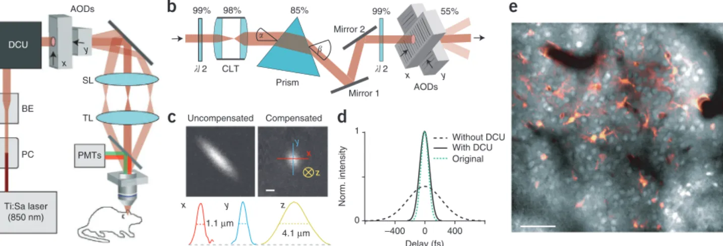
In vivo two-photon imaging using acousto-optic scanners Our first goal was to design an AOD-based two-photon scope suitable for in vivo application. We custom-built a micro-scope setup that uses a pair of crossed AODs for two-dimensional deflection of the laser beam (Fig. 1a). A critical issue in using AODs for two-photon excitation is that spatial and temporal dispersion cause laser focus deformation and pulse broadening, respectively. These effects can either be mitigated by using rela-tively long laser pulses (0.5–1.8 ps)14–16, albeit at the expense of
excitation efficiency, or they need to be compensated for with an additional diffractive element. Here we adopted a single-prism compensation approach17 and modified it to improve laser-beam
transmission and dispersion compensation over a large field of view (Fig. 1b). Compensation with the prism abolished elliptic deformation of the laser focus, as illustrated by imaging small fluorescent beads in the field of view center (Fig. 1c). Two half-wavelength (λ/2) waveplates before the prism and the first AOD, respectively, optimized laser beam polarization along the path-way and maximized transmission through prism (85%) and AOD pair (55%). In total, 45% of the incoming light was transmit-ted by the dispersion compensation unit (DCU) and the AODs. Additionally, a cylindrical telescope assured a round laser beam profile at the AOD aperture, compensating for the asymmetric light path through the prism (Online Methods).
Department of Neurophysiology, Brain Research Institute, University of Zurich, Zurich, Switzerland. Correspondence should be addressed to F.H. ([email protected]). Received 30 decembeR 2009; accepted 29 maRch 2010; published online 18 apRil 2010; doi:10.1038/nmeth.1453
high-speed
in vivo
calcium imaging reveals neuronal
network activity with near-millisecond precision
Benjamin F Grewe, Dominik Langer, Hansjörg Kasper, Björn M Kampa & Fritjof Helmchen
© 20 10 Nat ur e Amer ica, Inc. All r ights r eser ved.
We quantitatively characterized the spatial resolution by imaging 100-nm fluorescent beads (Supplementary Fig. 1). In the field of view center, lateral spatial resolution was uniform with 1.01 ± 0.14 µm and 1.01 ± 0.03 µm full-width at half- maximum (FWHM) in x and y direction, respectively; ellipti-city, defined as FWHM ratio along major and minor axis, was 1.0 (n = 4 beads, mean ± s.d.; ellipticity without compensation, 3.5). The resolution was limited by the resolvable number of spots of the AODs rather than the diffraction limit of the microscope objective (Online Methods). Axial resolution was 4.13 ± 0.14 µm FWHM (n = 4). As expected18, the focus was
elongated toward the field of view borders but ellipticity remained below 2 throughout the entire field of view (lateral and axial resolution remained below 2 µm and 6.5 µm FWHM, respectively; Supplementary Fig. 1). With the prism placed about 35 cm in front of the AODs, the DCU also compensated for the group delay dispersion in the entire optical path, restoring laser pulse width from ~570 fs without compensation to ~140 fs (130 fs original pulse width) (Fig. 1d). The total transmission efficiency of our microscope was ~25% at 850 nm wavelength, providing ample average laser power (up to 700 mW) below the microscope objective.
These optimizations rendered our system suitable for in vivo imaging and provided a field of view of up to 305 µm side length (40× objective). In living mice, we could readily image cell popu-lations in neocortical layer 2/3 (L2/3) down to 300 µm depth below the pia after multicell bolus loading2 with the fluorescent
calcium indicator Oregon Green BAPTA-1 (OGB-1) and counter-staining of astrocytes with sulforhodamine 101 (ref. 19) (Fig. 1e and Supplementary Movie 1).
high-speed calcium imaging from neuronal populations We next implemented a random-access scanning mode for fast calcium measurements. Although the 10-mm AOD aperture
size nominally supports point-to-point transitions within 15.4 µs (sound velocity 650 m s−1), the transition time could be
short-ened to 10 µs without any measurable effects15 (Online Methods).
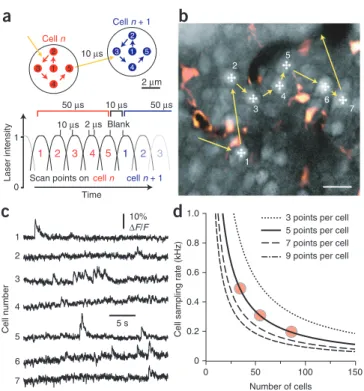
For frame scanning, we chose an additional 2-µs pixel dwell time, resulting in a frame acquisition time of 786 ms (256 × 256 pixel). For random-access scanning from cell populations, we used a longer signal integration time per neuron to increase fluorescence signals and improve SNR. To avoid stationary park-ing of the laser focus on the cell, which may cause photobleach-ing and cell damage15, we developed a random-access pattern
scanning (RAPS) mode, in which a predefined fixed spatial pat-tern of a few points is scanned on each neuron. In this study, we mainly used a five-point pattern that we scaled to match the cell size (Fig. 2a). After completing the pattern scan on one neuron, the laser focus jumped to the next neuron where again a pat-tern scan was started. On each cell, fluorescence signal was con-tinuously integrated during the pattern scan to maximize SNR. Signal integration was only blanked during the 10-µs transition period between individual neurons, resulting in a total effective dwell time of 50 µs per cell (Fig. 2a). Using five-point RAPS, we detected no signs of photodamage such as locally increased fluo-rescence15,20. Over cumulative scanning periods of up to 7 min,
neuronal morphologies were unaltered and basal fluorescence only slightly decreased by ~6%, comparable to galvanometric frame scanning (Supplementary Fig. 2).
Our RAPS mode enabled high-speed calcium imaging from neuronal populations. As an example, we measured spontane-ous calcium transients in 55 L2/3 neurons at 298 Hz (Fig. 2b). Spontaneous fluorescence transients with rapid onsets and amplitudes in the 5–20% range were clearly visible (Fig. 2c), suggesting that RAPS is well-suited to resolve action poten-tial–evoked calcium transients. In general, five-point RAPS can address 16,700 cell positions per second. Clearly, the number of sampled cells trades off against the effective sampling rate
a
c
PC SL TL PMTs Ti:Sa laser (850 nm) BE AODs DCU x y 1 0 400 0 –400 Delay (fs) Norm. intensity With DCU Without DCU Original Uncompensated Compensated y x z x y z 4.1 µm 1.1 µmb
Prism CLT �/ 2 AODs x y Mirror 1 Mirror 2 �/ 2 99% 98% 85% 99% 55%e
d
� �Figure 1 | AOD-based two-photon imaging of neocortical L2/3 neurons in vivo. (a) Schematic of the two-photon microscope setup. Laser intensity and beam size were adjusted with a Pockels cell (PC) and a variable beam expander (BE), respectively. After a DCU two orthogonal AODs were used for x–y scanning. (b) Schematic of the DCU consisting of a cylindrical lens telescope (CLT), two λ/2 waveplates and a single prism oriented at 45° angle to the AODs. Laser beam transmission percentage for each element is indicated. The CLT compensates for beam ellipticity caused by mismatch of the laser beam input and output angle (α and β). (c) Two-photon images of 500-nm fluorescent beads without (uncompensated) and with (compensated) the DCU. Intensity profiles along x, y and z direction are shown on the bottom with FWHM values indicated. Scale bar, 1 µm. (d) Laser pulse width measured with and without the DCU as well as the original pulse width at the laser output. (e) Two-photon image of a cell population stained with OGB-1 in L2/3 of mouse neocortex at 200 µm depth below the pia. Image of a astrocytes labeled with sulforhodamine 101 (red) is overlaid. Scale bar, 50 µm.
© 20 10 Nat ur e Amer ica, Inc. All r ights r eser ved.
| | | per cell (Fig. 2d): 16 neurons can be recorded at very high rate
(1 kHz), 30–40 cells at about 500 Hz, and groups of 100 cells at 167 Hz. Similar hyperbolic relationships between sampling rate and cell number hold for RAPS patterns with different numbers of points (Fig. 2d).
reliable spike detection with near-millisecond precision To directly examine whether single action potentials (1APs) can be detected and how precisely their timing might be inferred from the fluorescence traces, we combined RAPS with juxtacel-lular electrical recordings from individual neurons (Fig. 3a). We obtained simultaneous optical and electrical recordings from 10 L2/3 neurons in mouse barrel cortex using three different
cell sampling conditions (n = 3 at 181–228 Hz, groups of 72–91 cells sampled; n = 4 at 321–327 Hz, 51–55 cells sampled; n = 3 at 490 Hz, 34 cells sampled). In all cases 1AP-evoked calcium transients were clearly resolved (Fig. 3b,c). For a quantitative analysis of the reliability of spike detection, we developed an automated event detection algorithm based on a Schmitt trigger approach (Online Methods). From 293 total events that were mainly 1APs with a few doublets, 280 (95.5%) were correctly detected and 13 were missed (4.5% false negatives; 23 min cumu-lative recording time). Five events were incorrectly assigned (1.7% false positives). All action potential doublets (2–10 ms interspike interval) were detected, and 77% of them (17 out of 22) were correctly identified as doublets by the algorithm based on the expected integral of a 1AP-evoked calcium transient. The reliability of event detection was independent of whether spikes occurred spontaneously (1.5% false positives; 1/67 events) or whether they were evoked by air-puff whisker stimulation (1.8%; 4/221). To assess potential neuropil contamination of the somatic
a
c
1.0 0.8 0.6 0.4 0.2 0b
2 3 4 5 6 7 13 points per cell 5 points per cell 7 points per cell 9 points per cell
1 2 3 4 5 1 2 3 4 5 0 1 1 2 3 4 5 1 2 3 Cell n + 1 Cell n 10 µs 50 µs 2 µm Blank 2 µs
Scan points on cell n cell n + 1 Time
Cell sampling rate (kHz)
2 1 3 4 5 6 7 Cell number Number of cells 5 s 10% ∆F/F 100 50 0 10 µs 10 µs 50 µs Laser intensity 150
d
Figure 2 | Random-access pattern scanning from neuronal populations. (a) Principle of RAPS exemplified for a five-point pattern that is
sequentially scanned on two cell somata (top). Signal integration protocol for five-point RAPS (bottom). Cellular fluorescence signals are integrated over the entire five-point scan periods except for the 10 µs transition between cells. (b) Two-photon image of an L2/3 neuronal population labeled with OGB-1 (image of sulforhodamine 101–stained astrocytes (red) is overlaid; imaging depth, 198 µm). High-speed imaging (298 Hz sampling rate per cell) was performed using five-point RAPS targeted to 55 cells that were manually preselected from a reference image. RAPS transitions for seven example neurons are indicated. Scale bar, 20 µm. (c) Spontaneous fluorescence transients in the seven example neurons depicted in b. (d) Sampling rate per cell as a function of number of cells sampled and number of RAPS points per cell. Circles indicate the three regimes of sampling rates and cell numbers used in this study.
490 Hz n = 93 321–327 Hz n = 72 181–228 Hz n = 110 490 Hz 327 Hz 181 Hz 200 ms ∆t
b
c
d
a
2% 1.5 mV ∆F/F 5% ∆F/F 2 mV 5 s 5% 5 mV ∆F/F 2% 1.5 mV ∆F/F 5 ms 20 mse
f
0.2 s 2% ∆F/F CI = 15.6 ms CI = 10.4 ms CI = 4.8 ms –20 –10 0 10 20 Detection accuracy ∆t (ms)Figure 3 | Determining spike times from AOD-based optical recordings. (a) L2/3 cell population labeled with OGB-1 and sulforhodamine 101. A juxtacellular recording was obtained with a patch pipette (arrow) from the neuron marked with the five-point RAPS pattern (blue). Scale bar, 20 µm. (b) Simultaneous fluorescence measurement (top) and electrical recording (bottom) of one out of 51 neurons sampled at 327 Hz (neuron marked in a). Fluorescence trace was smoothed with a five-point box filter. (c) Example 1AP-evoked calcium transients for three different cells measured for 91 neurons sampled at 181 Hz (top), 51 neurons at 327 Hz (middle) and 34 neurons at 490 Hz (bottom; dashed box indicates the close-up shown in d). Blue traces are curve fits to the unfiltered raw fluorescence data. Dashed lines indicate zero lines. (d) Close-up of the initial phase of the calcium transient marked by the dashed box in c and the corresponding juxtacellular voltage recording (top). The onset of the fluorescence trace was fit with a rising exponential and an exponential decay (blue trace). Further zoom-in (bottom), with arrows marking the time difference, ∆t, between the spike time predicted from the onset fit and the actual spike time (0.85 ms in this case). (e) Average 1AP-evoked calcium transient pooled over all confirmed 1AP events independent of cell sampling rate (n = 250). (f) Summary histograms of the distribution of ∆t measured under the three sampling conditions. CI, 95% confidence intervals obtained from Gaussian fits (red curves; n is total number of events in each group).
© 20 10 Nat ur e Amer ica, Inc. All r ights r eser ved.
transients, we averaged failures to whisker stimulation, revealing small (~1%) fluo-rescence transients hidden in the noise (Supplementary Fig. 3). We confirmed a negligible neuropil contamination by direct comparison of fluorescence transients in somata and surrounding neuropil, demonstrating in particular apparent failures to evoke action poten-tials in the presence of large concomitant neuropil signals (Supplementary Fig. 3).
Each fluorescence transient detected was fitted in a two-step procedure with a model function composed of a single-exponential rise and a double-exponential decay. We chose two decay components because a rapid initial decay phase was apparent in the majority of transients (Fig. 3c,d and
Supplementary Fig. 4). In the first step, we
fitted the onset to determine the start of the event and the onset time constant. Then we fitted the entire calcium transient to obtain estimates of amplitudes and time constants for the two decay components (Online Methods). Results were independ-ent of cell sampling rate, and thus we pooled them. Onset time constant was on average 8.1 ± 0.5 ms (constrained to 2–30 ms,
n = 250 1AP events; mean ± s.e.m.).
Amplitudes (decay time constants) were 7.7 ± 0.2% (56 ± 3 ms) and 3.1 ± 0.1% (777 ± 80 ms) for the fast and slow component, respectively. The average peak amplitude of the fitted calcium transients was 7.2 ± 0.2%. Hence, our analysis revealed a stereo-typical 1AP-evoked calcium transient (Fig. 3e) that we used for subsequent analysis of spike trains. We defined the SNR as peak amplitude of the 1AP-evoked calcium transient divided by base-line noise. Basebase-line noise, defined as the s.d. of the fluorescence trace at rest, was low (2.1 ± 0.34% relative fluorescence change,
∆F/F) yielding SNR values of 2–5 (mean ± s.e.m., 3.5 ± 0.06;
Supplementary Fig. 4). We conclude that AOD-RAPS allows
reli-able detection of 1AP-evoked calcium transients.
Using the spike time estimate provided by the onset fit (Fig. 3d), we quantified how accurately spike times can be determined using RAPS. The time difference, ∆t, between the estimated and the actual spike time was 4.7 ± 0.6 ms, 1.1 ± 0.6 ms and 0.27 ± 0.35 ms for ~200 Hz, ~325 Hz and 490 Hz cell sampling rate, respectively (mean ± s.e.m.; n = 110, 72 and 93). The mean of the ∆t distribution thus reports spike time with an accuracy on the order of the sampling interval or better. To quantify the uncertainty in this spike time esti-mate, we constructed histograms of ∆t for all sampling conditions and determined the width of these distributions from Gaussian fits. The 95% confidence intervals (±2 s.d.) were 15.6, 10.4 and 4.8 ms for ~200 Hz, ~325 Hz and 490 Hz cell sampling rates, respectively (Fig. 3f). We conclude that AOD-RAPS reveals spike times with near-millisecond precision and 5–15 ms confidence intervals.
A peeling algorithm for automated spike-train reconstruction Calcium transients summate during higher-frequency spike trains (>1 Hz) because they last longer than action potentials.
Reconstruction of spike trains from noisy fluorescence traces thus is a chief goal of in vivo calcium imaging experiments1,21.
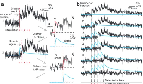
We developed a new spike-train reconstruction algorithm that is based on ‘peeling’ off 1AP-evoked calcium transients from the fluorescence trace until the entire spike train is uncovered (Online Methods). The principle of this automated algorithm is to (i) find the first event using the event detection algorithm, (ii) fit the onset to derive the timing of the first spike and (iii) subtract the stereotypical 1AP-evoked calcium transient placed at this time point from the fluorescence trace (Fig. 4a). These three steps are repeated until no additional events are found in the residual fluorescence trace (Fig. 4b and Supplementary
Movie 2). This procedure assumes an elementary 1AP-evoked
calcium transient and linear summation, which were reasonable approximations under our experimental conditions because dye saturation hardly affected even the largest transients analyzed (Supplementary Fig. 5).
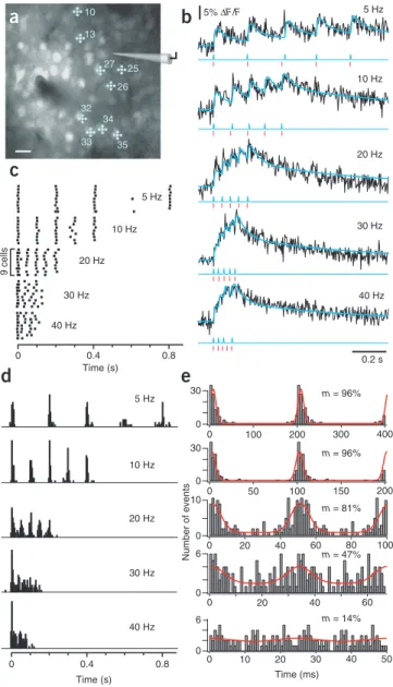
We first applied the peeling algorithm to investigate how well bursts of action potentials can be reconstructed from optical recordings using RAPS. To systematically induce spike trains in the 5–40 Hz frequency range, we directly stimulated neuronal populations with short electrical pulses22 through a patch-pipette
positioned in L2/3 (Fig. 5a). We increased stimulus intensity stepwise until a subpopulation of neurons reliably responded. At low frequencies, individual calcium transients were clearly discernible but they became increasingly harder to discriminate at higher frequencies (Fig. 5b). The largest fluorescence changes with 40 Hz stimulation were about 25–30%, which was still much lower than saturating fluorescence changes under our condi-tions (maximal relative fluorescence change (∆F/Fmax) = 93%;
a
200 ms Search event Detected spikes 5% ∆F/F 50 ms Fit onset Electrical stimulation 200 ms Search again Number of iteration 2 3 4 5 6 Number of iteration 1 2 3% ∆F/Fb
Subtract 1AP trace 3% ∆F/F Fit onset Subtract next 1AP trace Stimulation 1Figure 4 | Peeling algorithm for extracting spike trains from fluorescence transients. (a) Illustration of the automated peeling procedure. In the initial step, a first ‘event’ is detected using a customized Schmitt-trigger threshold routine. The onset of the detected calcium transient is fit within a short time window (red curve) in order to obtain a good estimate of the starting point of the event (red circle). Then a stereotypical 1AP-evoked calcium transient is placed with its start at this time point and is subtracted from the original fluorescence trace. Then the algorithm starts the next iteration on the resulting difference trace. (b) Example of the extraction of a train of five action potentials evoked by electrical stimulation at 10 Hz. For each iteration, the residual fluorescence trace as well as the accumulated trace of all 1AP-evoked calcium transients thus far extracted (blue trace) are depicted. After five iterations, no additional event was found in the residual fluorescence trace. At the bottom, detected spike times are shown together with the stimulus times.
© 20 10 Nat ur e Amer ica, Inc. All r ights r eser ved.
| | | Online Methods). For each trace, we used the peeling algorithm
to reconstruct a model trace of accumulated calcium transients and to extract a raster plot of the detected spike times. A sum-mary raster plot for one experiment (Fig. 5c) as well as cumula-tive spike time histograms for five experiments (Fig. 5d; n = 29 cells) indicate that the imposed burst frequency is well extracted up to 20 Hz, but it cannot be clearly resolved at higher frequen-cies. This finding was corroborated by an additional phase analy-sis, in which we generated histograms of the spiking phase within the stimulus cycles for all spikes in the train (Fig. 5e). The widths of Gaussian fits to these phase histograms were on the order of 5 ms and the modulation was high (>80%) up to 20 Hz stimulus frequency, 47% at 30 Hz, but strongly reduced at 40 Hz (Fig. 5e). We conclude that AOD-RAPS permits reconstruction of spike times for bursts of action potentials with frequencies up to 20 Hz and with confidence intervals on the order of 20 ms.
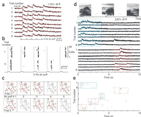
spatiotemporal dynamics of sensory-evoked spiking activity To directly determine whether the combination of AOD-RAPS and peeling analysis facilitates in vivo studies of neural coding
on a fast time scale, we measured population spiking dynamics in primary sensory areas of the neocortex. First, we recorded population response in the barrel cortex while repetitively stim-ulating the contralateral whiskers with a 5-Hz train of 5 air puffs (Fig. 6a). The sensory-evoked responses in individual neurons as well as in the sampled population showed trial-to-trial vari-ability with apparent failures to respond to particular stim-uli during the air-puff trains (Fig. 6b,c and Supplementary
Fig. 6). The cell sampling rate (298 Hz; 95% confidence
inter-val, 10.4 ms) was sufficient to resolve differences in global latency of population responses, which were in the range of 10–20 ms and may have originated from distinct states of ongoing activity at the time of stimulation (Fig. 6b). For example, the population response to the first stimulus was significantly delayed in trial 1 compared to the response in trial 5 (mean onset difference, 9.1 ms; P < 0.001). Notably, the spatial dynamics of population activity within a few tens of milliseconds after individual air puffs could be visualized in movies based on the automatically detected spike times and taking into account the confidence interval of spike time reconstruction (Supplementary Movie 3).
Second, we measured spiking activity in mouse primary vis-ual cortex in response to the presentation of a natural movie of 10 s duration. In three experiments we found several neu-rons that responded consistently during brief epochs (around 1–2 s duration) at particular time periods during the movie (Fig. 6d), which is in agreement with electrophysiological find-ings23. With the peeling algorithm, we extracted spike raster
plots, revealing within-epoch variability of spike numbers and spike timing (Fig. 6e). These examples demonstrate that AOD-RAPS resolves spatiotemporal dynamics of sensory-evoked spiking activity in neocortical neural networks on a subsecond time scale.
a
b
d
40 Hz 30 Hz 20 Hz 10 Hz 5 Hzc
0.2 se
40 Hz 30 Hz 20 Hz 10 Hz 5 Hz 9 cells m = 47% m = 14% m = 96% m = 81% m = 96% 30 0 30 0 10 Number of events 0 6 0 0 100 200 300 400 0 50 100 150 200 0 20 40 60 80 100 0 20 40 60 0 10 20 30 40 50 6 0 Time (ms) 5% ∆F/F 40 Hz 30 Hz 20 Hz 10 Hz 5 Hz 10 13 25 26 35 34 33 32 27 Time (s) Time (s) 0 0.4 0.8 0 0.4 0.8Figure 5 | Spike train reconstruction for bursts with different action potential frequency. (a) Two-photon image of a L2/3 neuronal population in mouse barrel cortex labeled with OGB-1. Trains of 5 electrical stimuli at variable frequency were applied extracellularly through a micropipette. In this example, 9 out of 40 neurons sampled at 416 Hz using five-point RAPS responded reliably to the electrical stimulation. Responding cells are marked with cell numbers and schematic scan pattern. Scale bar, 20 µm. (b) Example fluorescence transients for stimulus frequencies of 5–40 Hz from a neuron in another experiment. Blue traces are model traces reconstructed by the peeling algorithm. Extracted spike times (blue) are shown together with the stimulus times (red). (c) Raster plots of the spiking responses to stimulation at different frequencies for the nine neurons marked in a, extracted using the peeling algorithm. The length of individual ticks reflects the confidence interval of spike detection from 1AP-evoked calcium transients. (d) Summary histograms of reconstructed spiking responses to stimulation at different frequencies (n = 29 cells from three experiments; RAPS rates, 278–416 Hz). Note that the stimulus frequency is still apparent in the 20-Hz histogram. (e) Phase analysis of spiking responses to the burst stimulation. Spike times were recalculated modulo the duration of one stimulus cycle, and histograms were accumulated, revealing the phase relationship of detected spikes relative to the stimulus interval. For better visibility, two cycles containing the same datasets are shown side by side. Red traces are curve fits with a Gaussian function, revealing peak amplitude Amax and basal offset Amin. Values for the modulation, calculated as m = (Amax − Amin)/(Amax + Amin), are indicated.
© 20 10 Nat ur e Amer ica, Inc. All r ights r eser ved.
discussion
Here we overcame a major limitation of optical recordings from neuronal populations by demonstrating two-photon imaging of neural networks in the intact brain with unprecedented temporal resolution. Compared to previous in vivo experiments using galvanometer-based frame scanning at 1–30 Hz3,4,6,8, our
AOD-based scanning system achieved cell sampling rates up to 500 Hz, gaining a factor of 10–100 in temporal resolution. Previous AOD-based two-photon microscopes have achieved similar scan-ning speed but they were mainly used for calcium imaging of neuronal dendrites in brain slices14–16. Here our aim was to design
a relatively simple microscope that efficiently delivers short laser pulses to the intact brain and thus enables in vivo application. All main microscope components are readily available, and beam path alignment is straightforward, with the DCU prism and the AODs as key adjustable components. Alternatively, fast cell sam-pling might be achievable with special galvanometric line-scan techniques12,24. However, these techniques still waste some scan
time on background areas and lack the flexibility to scan arbitrary patterns; it is currently unclear whether they can provide suffi-cient SNR for measuring population activity in vivo.
Our AOD-RAPS mode extends previous random-access scan-ning modes14,15. By scanning a small point pattern on each
individual neuron, we achieved a high SNR while minimizing photobleaching and photodamage. The resulting SNR of about 3.5 for 1AP-evoked calcium transients enabled us to detect spikes with high reliability (>95%) and with near-millisecond preci-sion. Our ability to simultaneously attain high SNR and high cell sampling rates is explained by the fact that the effective dwell times per cell are similar to those of slower frame scanning systems4,6–8,25.
The high temporal resolution was particularly beneficial for
characterizing 1AP-evoked calcium transients in detail. We con-firmed peak amplitudes of 7–8% for 1AP-evoked somatic calcium transients4,8 but also found that their decay typically consisted of a
fast and a slow component. The initial fast component (<100 ms) might be undersampled with low-speed systems, which could partially explain difficulties to detect 1APs.
Various methods have been explored for inferring spike trains from calcium indicator fluorescence measurements, including deconvolution techniques26, template matching6,7, model-based
fitting25 and sequential Monte Carlo methods27. With our new
iterative ‘peeling’ algorithm, we could resolve spike times for spikes spaced as close as 40–50 ms apart. The peeling algorithm is generally applicable and computationally simple. In its simplest version described here the algorithm assumes a stereotype cal-cium transient and neglects dye saturation. Various extensions are possible though; for example, different 1AP transient waveforms are likely to apply for different cell types and for large calcium changes the reduction in the fluorescence transient amplitude with increasing dye saturation could be incorporated.
Although in this work we collected in vivo measurements in two dimensions, our approach should be extendable to three dimen-sions using either mechanical z-dimension scanning5 or chirped
acoustic waves in a series of AODs16,28. We expect that high-speed
measurements could be especially beneficial for analyzing spike sequences in specific neuronal subsets after slower screening of large populations for relevant subensembles. Retrograde labeling techniques and transgenic mice with fluorescent protein expres-sion could be particularly helpful for guiding measurements to specific cell types. Moreover, the use of genetically encoded cal-cium indicators9–11,29 with high-speed calcium imaging opens new
opportunities for repeated long-term functional interrogation
a
b
Time 20% ∆F/F . . . .d
0.1 s Cellsc
5 Hz air puff 5 Hz air puff Trial number Trial number 0.2 s Trial number Trial number 1 5 0 5 10 Trial 1 Trial 5 Air puff # 1 2 3 4 5 0 5 10e
10% ∆F/F 1 56 Cell 25 4 6 8 2 1 3 5 7 8 1 8 1 8 1 Time (s) Time (s) Figure 6 | Subsecond trial-to-trial variability ofsensory-evoked responses in mouse neocortex. (a) Example calcium transients in an L2/3 neuron of mouse barrel cortex in response to stimulation with a 5-Hz train of air puffs (five-point RAPS at 298 Hz, 56 neurons sampled, eight consecutive trials). Model traces reconstructed by the peeling algorithm (red) indicate detected action potentials, including putative evoked doublets and triplets. (b) Population raster plots for two selected trials (all trials are shown in supplementary Fig. 6). Vertical dashed lines indicate air-puff stimulation triggers. Tick length reflects confidence interval for spike reconstruction (red ticks indicate spikes for the neuron shown in a). (c) Snapshots of the subpopulations activated by an air-puff train for trial 1 and 5. Active cells that elicited at least one spike within a 50-ms time window after a stimulus are marked in red (arrow points to example cell in a). (d) Three chronological scenes from a 10-s natural movie that was repeatedly presented to the contra-lateral eye (top). Example fluorescence transients from two L2/3 neurons in mouse visual cortex evoked by eight consecutive presentations of the movie (two different five-point RAPS experiments at 278 Hz and 309 Hz). Response epochs are indicated
by a blue and a red box. Overlaid colored traces in boxes are model traces reconstructed by the peeling algorithm. (e) Raster plots of reconstructed spiking responses to eight repeats of the movie presentation for five neurons that showed reliable activation during specific epochs of the movie (indicated by boxes).
© 20 10 Nat ur e Amer ica, Inc. All r ights r eser ved.
| | | of neuronal networks. A particular challenge will be to perform
high-speed AOD-based calcium imaging in awake animals, where motion artifacts need to minimized or corrected for30,31.
The combination of fast optical recording and automated spike train reconstruction will facilitate studies of various aspects of neural coding. First, a better characterization of bursting behav-ior of cortical neurons should be possible, which appears to be enhanced during wakefulness25,32. Second, phase-relationship
studies of action potential firing with respect to global neuronal oscillations such as hippocampal 4–10 Hz theta oscillations33
should be feasible. Third, high-speed imaging should enable detailed analysis of the variability of absolute (in a cell) and relative (between cells) spike timing, addressing the question of temporal versus rate coding34. Finally, recording a few neurons
at highest speed (0.5–1 kHz) may allow optical investigation of network plasticity that is likely to be ruled by relative spike timing differences on the order of a few ten milliseconds35,36. AOD-based
in vivo imaging thus is likely to become a versatile technique for studying fundamental principles of neural information process-ing in microcircuits of the brain.
methods
Methods and any associated references are available in the online version of the paper at http://www.nature.com/naturemethods/. Note: Supplementary information is available on the Nature Methods website. AcknoWledgments
We thank H. Lütcke, D. Margolis and H. Grewe for comments on the manuscript. This work was supported by a Forschungskredit of the University of Zurich (B.F.G.), and by grants to F.H. from the Swiss National Science Foundation (3100A0-114624), the EU-FP7 program (SPACEBRAIN project 200873) and the Swiss SystemsX.ch initiative (project 2008/2011-Neurochoice).
Author contriButions
B.F.G. and F.H. designed and optimized the AOD-based microscope system; B.F.G. built the microscope; B.F.G. and D.L. designed the data acquisition software; B.F.G. and H.K. designed the AOD control electronics; B.F.G. performed all in vivo
experiments; F.H. developed the peeling algorithm for spike train reconstruction; B.M.K. helped with animal preparation and in vivo experiments; B.F.G. and F.H. analyzed the data and wrote the manuscript.
comPeting FinAnciAl interests
The authors declare no competing financial interests.
Published online at http://www.nature.com/naturemethods/.
reprints and permissions information is available online at http://npg.nature. com/reprintsandpermissions/.
1. Grewe, B.F. & Helmchen, F. Optical probing of neuronal ensemble activity.
Curr. Opin. Neurobiol.19, 520–529 (2009).
2. Stosiek, C., Garaschuk, O., Holthoff, K. & Konnerth, A. In vivo two-photon calcium imaging of neuronal networks. Proc. Natl. Acad. Sci. USA100, 7319–7324 (2003).
3. Ohki, K., Chung, S., Ch’ng, Y.H., Kara, P. & Reid, R.C. Functional imaging with cellular resolution reveals precise micro-architecture in visual cortex.
Nature433, 597–603 (2005).
4. Kerr, J.N.D., Greenberg, D. & Helmchen, F. Imaging input and output of neocortical networks in vivo. Proc. Natl. Acad. Sci. USA102, 14063–14068 (2005).
5. Göbel, W., Kampa, B.M. & Helmchen, F. Imaging cellular network dynamics in three dimensions using fast 3D laser scanning. Nat. Methods4, 73–79 (2007).
6. Sato, T.R., Gray, N.W., Mainen, Z.F. & Svoboda, K. The functional microarchitecture of the mouse barrel cortex. PLoS Biol.5, e189 (2007). 7. Kerr, J.N. et al. Spatial organization of neuronal population responses in
layer 2/3 of rat barrel cortex. J. Neurosci.27, 13316–13328 (2007).
8. Rochefort, N.L. et al. Sparsification of neuronal activity in the visual cortex at eye-opening. Proc. Natl. Acad. Sci. USA106, 15049–15054 (2009). 9. Wallace, D.J. et al. Single-spike detection in vitro and in vivo with a
genetic Ca2+ sensor. Nat. Methods5, 797–804 (2008).
10. Tian, L. et al. Imaging neural activity in worms, flies and mice with improved GCaMP calcium indicators. Nat. Methods6, 875–881 (2009). 11. Lütcke, H. et al. Optical recording of neuronal activity with a
genetically-encoded calcium indicator in anesthetized and freely moving mice. Front. Neural Circuits4, 9 (2010).
12. Lillis, K.P., Eng, A., White, J.A. & Mertz, J. Two-photon imaging of spatially extended neuronal network dynamics with high temporal resolution. J. Neurosci. Methods172, 178–184 (2008).
13. Nikolenko, V. et al. SLM Microscopy: Scanless two-photon imaging and photostimulation with spatial light modulators. Front. Neural Circuits2, 5 (2008). 14. Iyer, V., Hoogland, T.M. & Saggau, P. Fast functional imaging of single
neurons using random-access multiphoton (RAMP) microscopy. J. Neurophysiol.95, 535–545 (2006).
15. Otsu, Y. et al. Optical monitoring of neuronal activity at high frame rate with a digital random-access multiphoton (RAMP) microscope. J. Neurosci. Methods173, 259–270 (2008).
16. Reddy, G.D., Kelleher, K., Fink, R. & Saggau, P. Three-dimensional random access multiphoton microscopy for functional imaging of neuronal activity.
Nat. Neurosci.11, 713–720 (2008).
17. Zeng, S. et al. Simultaneous compensation for spatial and temporal dispersion of acousto-optical deflectors for two-dimensional scanning with a single prism. Opt. Lett.31, 1091–1093 (2006).
18. Kremer, Y. et al. A spatio-temporally compensated acousto-optic scanner for two-photon microscopy providing large field of view. Opt. Express16, 10066–10076 (2008).
19. Nimmerjahn, A., Kirchhoff, F., Kerr, J.N. & Helmchen, F. Sulforhodamine 101 as a specific marker of astroglia in the neocortex in vivo. Nat. Methods1, 31–37 (2004).
20. Koester, H.J., Baur, D., Uhl, R. & Hell, S.W. Ca2+ fluorescence imaging
with pico- and femtosecond two-photon excitation: signal and photodamage. Biophys. J.77, 2226–2236 (1999).
21. Göbel, W. & Helmchen, F. In vivo calcium imaging of neural network function. Physiology (Bethesda)22, 358–365 (2007).
22. Histed, M.H., Bonin, V. & Reid, R.C. Direct activation of sparse, distributed populations of cortical neurons by electrical microstimulation.
Neuron63, 508–522 (2009).
23. Goard, M. & Dan, Y. Basal forebrain activation enhances cortical coding of natural scenes. Nat. Neurosci.12, 1444–1449 (2009).
24. Göbel, W. & Helmchen, F. New angles on neuronal dendrites in vivo.
J. Neurophysiol.98, 3770–3779 (2007).
25. Greenberg, D.S., Houweling, A.R. & Kerr, J.N. Population imaging of ongoing neuronal activity in the visual cortex of awake rats. Nat. Neurosci.11, 749–751 (2008).
26. Yaksi, E. & Friedrich, R.W. Reconstruction of firing rate changes across neuronal populations by temporally deconvolved Ca2+ imaging. Nat.
Methods3, 377–383 (2006).
27. Vogelstein, J.T. et al. Spike inference from calcium imaging using sequential Monte Carlo methods. Biophys. J.97, 636–655 (2009). 28. Vucinic, D. & Sejnowski, T.J. A compact multiphoton 3D imaging system
for recording fast neuronal activity. PLoS One2, e699 (2007).
29. Mank, M. et al. A genetically encoded calcium indicator for chronic in vivo
two-photon imaging. Nat. Methods5, 805–811 (2008).
30. Dombeck, D.A., Khabbaz, A.N., Collman, F., Adelman, T.L. & Tank, D.W. Imaging large-scale neural activity with cellular resolution in awake, mobile mice. Neuron56, 43–57 (2007).
31. Greenberg, D.S. & Kerr, J.N. Automated correction of fast motion artifacts for two-photon imaging of awake animals. J. Neurosci. Methods176, 1–15 (2009). 32. de Kock, C.P. & Sakmann, B. Spiking in primary somatosensory cortex
during natural whisking in awake head-restrained rats is cell-type specific.
Proc. Natl. Acad. Sci. USA106, 16446–16450 (2009).
33. Hartwich, K., Pollak, T. & Klausberger, T. Distinct firing patterns of identified basket and dendrite-targeting interneurons in the prefrontal cortex during hippocampal theta and local spindle oscillations. J. Neurosci. 29, 9563–9574 (2009).
34. Kostal, L., Lansky, P. & Rospars, J.P. Neuronal coding and spiking randomness. Eur. J. Neurosci.26, 2693–2701 (2007).
35. Caporale, N. & Dan, Y. Spike timing-dependent plasticity: a Hebbian learning rule. Annu. Rev. Neurosci.31, 25–46 (2008).
36. Kampa, B.M., Letzkus, J.J. & Stuart, G.J. Dendritic mechanisms controlling spike-timing-dependent synaptic plasticity. Trends Neurosci.30, 456–463 (2007). © 20 10 Nat ur e Amer ica, Inc. All r ights r eser ved.
pair of AODs. Optical components were mounted on a vertical X95 profile column (X95-750; Linos) attached to an x-y motorized stage (KT 310; Feinmess) to permit lateral movements of the microscope. Laser pulses of about 130-fs width at 850 nm wavelength were pro-vided by a Ti:sapphire laser system (>3 W maximum average power; Chameleon Ultra II; Coherent). Laser intensity was modulated with a Pockels cell (model 350-80; Conoptics) and the laser beam was 3× expanded with a variable beam expander (S6ASS2075, Silloptics). Owing to its intrinsic divergence, the laser beam further expanded along the 4.5-m optical path to a beam diameter of 7.9 mm at the AOD aperture (full 1/e2 width). Scan lens (achromatic, f
SL = 300 mm,
NIR coating; Thorlabs) and tube lens (achromatic, fTL = 180 mm; Olympus) were chosen to realize a maximum scanning field of 305 µm × 305 µm under a 40× objective. All experiments were performed with a water-immersion objective (40× LUMPlanFl/IR, numerial aperture (NA) 0.8, back aperture 7.2 mm; Olympus). The 0.6× demagnification of scan- and tube-lens telescope resulted in a beam diameter of 4.9 mm at the objective’s back aperture, which hence was underfilled. The microscope objective and the fluores-cence detection system were mounted on a motorized z-dimension stage (PMT 160 DC; Feinmess). Green and red fluorescence signals were detected in two emission channels using photomultipliers (R6357; Hamamatsu), digitized at 20 MHz and digitally integrated using an FPGA board (PXI-8713R; National Instruments). Scan signals for the AODs, including the RAPS mode, and data acquisi-tion were controlled with software custom-written in the LabView environment (National Instruments).
We chose two orthogonally mounted AODs (DTSXY-A12-850, AAoptoelectronics) optimized for high transmission and an adequate resolution over a large field of view (FOV) (10 mm active aperture, 47 mrad total scan angle Q, ~55% transmission at λ = 850 nm). For a Gaussian laser beam with full 1/e2 width D the maximum number
of resolvable spots per axis is given by N = π/4 × Q × D/λ (see, for example, ref. 18). With slightly underfilled AOD aperture (D = 7.9 mm), we calculate 342 resolvable spots, and given our FOV of 305 µm, a theoretical focal spot size of about 0.9 µm, in close agree-ment with the results from the bead measureagree-ments (Suppleagree-mentary
Fig. 1). We thus conclude that the small scan angle of the AODs
rather than the diffraction limit of the underfilled objective, which would yield about 0.5 µm resolution, is the major limiting factor for spatial resolution in our microscope. Because efficient in vivo imag-ing of cell bodies over a substantial FOV size was our primary goal, this spatial resolution was adequate for our purposes.
As reported in another study15, the transition time of AODs can
be substantially shortened compared to the theoretical value. The reason is that within about 66% of the nominal transition time (given by the passage time of the sound wave across the full beam diameter at the AOD aperture) more than 90% of the laser power is redirected to the new position, meaning that <1% excitation remains at the original position. We adopted this approach and used a 10-µs transition time between scan angles, which is 82% of the nominal transition time for our 7.9-mm beam size at the AOD aperture (12.2 µs; sound velocity 650 m s−1) and 66% of the
nominal transition time for the fully filled AOD aperture (15.4 µs). In agreement with the previous report15, we did not observe any
measurable effect on image quality.
the first AOD17,37. By tuning the laser beam’s incident angle on
the prism to the theoretical value of 53°, we could counterbalance spatial dispersion effect nearly perfectly for the center of the FOV (Supplementary Fig. 1). The appropriate distance of the prism from the first AOD for minimizing laser pulse width after the AODs was about 35 cm, as determined by pulse length measurements with a frequency-resolved optical gating (FROG) device (Grenouille; Swamp Optics; the beam profiler option of the FROG was also used for measurement of the beam diameter along the optical path). Two λ/2 waveplates (RZ-1/2-850; Thorlabs/OFR) were used to appropriately turn laser beam polarization for maximizing light transmission. A cylindrical lens telescope composed of two plano-convex cylindrical lenses (f1 = 100 mm, f2 = 50 mm, achromatic, N-BK7, near-infrared (NIR) coating; Thorlabs) was necessary to counterbalance the unidirectional demagnification caused by the asymmetric beam pathway of the laser beam through the prism (beam ellipticity of 0.61 if not corrected).
Mouse preparation and fluorescence labeling. All animal
proce-dures were carried out according to the guidelines of the Center for Laboratory Animals of the University of Zurich and were approved by the Cantonal Veterinary Office. Wild-type mice (16–28 days old) were anesthetized with urethane (1.2-1.5 g kg−1 of body weight,
intraperitoneally) or isoflurane (1–2% in oxygen). A craniotomy above the somatosensory cortex was prepared as described previ-ously4,19. The dura was carefully removed, and the exposed cortex
was superfused with normal rat Ringer (NRR) solution (135 mM NaCl, 5.4 mM KCl, 5 mM Hepes, 1.8 mM CaCl2; pH 7.2 with NaOH). To dampen heartbeat- and breathing-induced motion, the cranial window was filled with agarose (type III-A, Sigma; 1% in NRR) and covered with an immobilized glass cover slip.
Cell populations were labeled in superficial neocortical layers with the calcium indicator Oregon Green BAPTA-1 (Molecular Probes, Invitrogen) using the multicell bolus loading technique2,38.
Briefly, 50 µg of the membrane-permeant acetoxymethyl (AM) ester form of OGB-1 were dissolved in DMSO plus 20% Pluronic F-127 (BASF) and diluted in NRR to a final concentration of about 1 mM. This solution was pressure-ejected into neocortical layer 2/3 in barrel cortex or visual cortex using a micropipette4.
Brief (10 min) application of sulforhodamine 101 (50 µM in NRR) to the exposed neocortical surface resulted in labeling of the astrocytic network19.
Calcium imaging and electrophysiology. Frame scanning with
10-µs pixel-to-pixel transition time and 2-µs pixel dwell times was used to obtain overview images of neuronal populations in L2/3. Groups of cell somata in the focal plane were manually selected for random-access scanning, and cell positions were saved. Fluorescence signals were recorded using RAPS to maximize SNR while minimizing bleaching effects. In this study, we used a cross-like five-point pattern with point-to-point distance of 1.5 µm so that all points were contained within the somatic area. The total scan time per cell was 60 µs with an effective on-cell signal integration time of 50 µs (Fig. 2). The stability of fluorescence levels during five-point RAPS was evaluated by measuring the baseline fluorescence from neurons that were imaged in 21 imaging
© 20 10 Nat ur e Amer ica, Inc. All r ights r eser ved.
3 measurements; Supplementary Fig. 2). Neighboring control neurons, which were not included in the RAPS recording but only rarely imaged using frame scans every 30 s, showed stable fluo-rescence intensity (97.4 ± 2.5%, n = 10 cells). The observed fluo-rescence decrease was not specific to five-point RAPS as a similar decrease was seen for neurons that were imaged using galvanomet-ric frame scanning with a standard two-photon microscope using similar laser power and total dwell time per cell (decrease to 91.3 ± 0.9%; n = 25 cells from 3 measurements; Supplementary Fig. 2). To evaluate potential contamination of somatic fluorescence transients by neuropil signals21, we performed five-point RAPS
recordings of air-puff–evoked fluorescence transients from cell somata and simultaneously from the surrounding neuropil (Supplementary Fig. 3). Somatic and neuropil signals were inde-pendent from each other, showing all possible combinations of evoked signals and apparent failures. Notably, apparent failures to evoke action potentials were found in cases of large activation of the surrounding neuropil indicating a rather small contamination by neuropil. This conclusion was supported by identified failure events (no action potential evoked with air-puff stimulation) that could be identified in our combined electrical and optical recording dataset. Averaging fluorescence traces for these failures revealed signals with 1.2 ± 0.3% amplitude that might represent small contamination by neuropil (Supplementary Fig. 3). Because these events are typically buried in noise and their integral is far below 50% of the expected integral for a 1AP-evoked transient, they will not be recognized by the peeling algorithm or discarded (see below).
Juxtacellular recordings were obtained from OGB-1–loaded L2/3 neurons. Cells were visually targeted in the frame scan mode of the AOD two-photon microscope. Borosilicate glass pipettes with open tip resistances of 4–8 MΩ were filled with extracellular solu-tion containing Alexa Fluor 594 (50 µM) for pipette visualization. Electrical signals were recorded with an Axoclamp 2-B amplifier (Axon Instruments) and digitized at 10 kHz with a PXI-6229 data acquisition card (National Instruments). For electrical stimulation experiments 200-µs pulses (0.1–1 mA) were delivered through patch pipettes placed within the imaging area22. Sensory stimulation of the
barrel cortex and the visual cortical areas was performed by 30-ms air puffs to the whiskers on the contralateral side of the face and by presenting a 10-s natural contrast movie to the mouse’s contralateral eye (movie 161 from a published database39), respectively. Data analysis. Somatic fluorescence signals were expressed as
relative fluorescence changes (∆F/F) after subtraction of the back-ground, which was determined from a position inside a blood vessel lumen. All fluorescence traces in the figures are unfiltered except for the trace in Figure 3b, which was filtered with a five-point box filter to improve visibility of the compressed trace. Fluorescence traces and electrophysiological signals were analyzed with IGOR Pro software (Wavemetrics Inc.). Below we describe in detail the automated analysis routines that we developed for event detection, onset and decay fitting, and reconstruction of spike trains from superimposed fluorescence transients.
Event detection. Events were detected using a Schmitt trigger
approach with additional criteria. A Schmitt trigger searches point
implementation we used +2 s.d. of the baseline noise (4.2%) as high threshold, −1 s.d. (−2.1%) as low threshold and typically 70 ms as minimum event length. To render our algorithm less sensitive to drifts in the baseline, we applied the Schmitt trigger in a sliding window approach in which a baseline was fit with a linear regression in a 0.4-s window before the current position. Offset and slope of this baseline were taken into account for the Schmitt trigger evaluation. An event detected by the Schmitt trig-ger had to fulfill two additional criteria to be accepted. First, the integral of the baseline-corrected fluorescence trace in the event window (from passing high threshold to falling below low thresh-old) was calculated and compared to the integral of a reasonable expectation of a 1AP-evoked calcium transient. The event was only accepted if the ratio of these two integrals was above 0.5, indicating a high probability that at least one action potential has occurred. The rounded ratio number was also used to estimate the number of nearly simultaneously occurring action potentials, that is, a ratio of between 1.5 and 2.5 indicated the occurrence of a doublet. As last criterion, a similar integral comparison was performed on a shorter time window (within 40–60 ms after high-threshold crossing) to ensure that only events with rather sharp onset, as expected for action potential-evoked calcium transients40, were
selected. For accepted events, the routine returned the time point of high-threshold crossing as an initial guess of the event start.
Onset fit. Onsets of detected events were fitted within a window
of ± 40 ms (±60 ms for ~200 Hz cell sampling rate) around the initial guess t0 from the event detection routine with the follow-ing function: f t A t t f t t t t t onset onset ( ) = (1 e e for > ( ) = on 0 − ( (− − 0)/t ) ( (− − 0)/ )t1 00 fort t≤ 0
Before fitting, baseline offset and linear drift were subtracted from the trace segment. An exponentially decaying component (τ1 set to a fixed value of 70 ms) was included because fluorescence traces typically already started to decay within the chosen time window. The free parameters were t0, τon and A. t0 was constrained to the fit window and τon was constrained to 2–30 ms to avoid artificially steep or shallow onsets. The major goal of onset fitting was to obtain a good estimate of t0.
Fitting of entire 1AP-evoked fluorescence transients. The
high-speed measurements revealed that the decay of action potential– evoked somatic calcium transients in most cases could not be well described with a single-exponential curve. Several decay components may be expected as the spatiotemporal dynamics of intracellular cal-cium concentration in the soma is governed by multiple processes, including calcium diffusion and buffering in the cytosol and in the nucleus as well as uptake and extrusion mechanisms41. We therefore
used a calcium transient waveform with sharp exponential onset and a slower double-exponential decay to fit the fluorescence trace:
fCa( )t = 1−e− −(t t0)tonA1e− −(t t0)t1+A2e− −(t t0)t2foor for Ca t t f t t t > = ≤ 0 0 0 ( ) (1) (1) (2) (2) © 20 10 Nat ur e Amer ica, Inc. All r ights r eser ved.
0
For the juxtacellular recordings, spike times ts were determined as the time point of the positive peak of the extracellular spike, which coincides with the steepest rise in membrane potential during the action potential. As the evoked calcium influx occurs during the repolarizing action potential phase42, which is about
1 ms after the steepest rise in neocortical pyramidal neurons43,
we calculated the time difference between optical estimate and actual spike time as ∆t = t0 − (ts + 1 ms).
Peeling algorithm for automated spike train reconstruction.
To reconstruct complex spike trains, we developed a generalized approach for automatically extracting spike times from arbitrary fluorescence traces. We assumed that each fluorescence trace represents the linear summation of 1AP-evoked calcium tran-sients with a stereotypical waveform. This assumption is justi-fied because the largest transients under our conditions (25–30%
∆F/F) were little affected by dye saturation (see below). The
prin-ciple of the algorithm is to iteratively subtract (‘peel off ’) an 1AP-evoked calcium transient waveform at the detected event times from the fluorescence trace until a model trace of the compound calcium transients is reconstructed and a noisy residual trace remains (Fig. 4 and Supplementary Movie 2). In our implemen-tation we always used the estimate of the 1AP-evoked calcium transient waveform from the combined electrical (juxtacellular) and optical recordings for subtraction (Fig. 3e). To accommodate slight cell-to-cell variations in calcium transient amplitude, this waveform was scaled in some experiments (0.7–1.3 scale factor). To prevent subtraction of erroneous events we performed an ‘integral check’: subtraction of the 1AP-evoked calcium transient was only accepted if it did not produce a negative integral in the residual trace (more than 50% of the negative of the integral of a 1AP-evoked transient); otherwise the subtraction was undone and the procedure moved on to the next event found. For accepted events the algorithm ‘jumped back’ on the trace (typically 200 ms) after waveform subtraction and started the search for the next event. The peeling algorithm is computationally simple and can be implemented effectively as a fast procedure. We used a macro implementation in the IGOR software (Wavemetrics).
Modeling of summation of [Ca2+]
i transients. To assess the
amount of dye saturation during repetitive electrical stimula-tion (Fig. 5), we first experimentally determined the maximal relative fluorescence change, ∆F/Fmax, under our experimental conditions. After the usual OGB-1 staining procedure we deliber-ately destroyed L2/3 neurons by applying strong electrical shocks through a local micropipette while simultaneously monitoring fluorescence changes. Analysis of neurons, for which cell damage was obvious as a sudden fluorescence increase to a stable ceiling value, yielded an average ∆F/Fmax value of 93 ± 15% (n = 10 cells; mean ± s.d). Together with reasonable assumptions of 50 nM for the resting intracellular calcium concentration, [Ca2+]
rest44,45 and of 200 nM for the dissociation constant Kd of
OGB-1 (ref. 45), we thus could convert the average 1AP-evoked
∆F/F transient into an intracellular concentration transient of free
calcium, [Ca2+]
i transient using the standard single-wavelength
conversion equation:
max
1−
( )
(∆F F/ )
The calculated 1AP-evoked [Ca2+]
i transient had a peak
amplitude of about 10 nM, which is consistent with previous calibrated [Ca2+]
i measurements from neocortical neurons46
(Supplementary Fig. 5). We then calculated [Ca2+]
i elevations
during burst stimulation at different frequency by assuming lin-ear superposition of the individual [Ca2+]
i transients. Despite
the linear summation, compound [Ca2+]
i traces seemed to show
some degree of saturation; however, this misleading impression was due to the combination of the finite onset of the transient and the fast initial decay component (Supplementary Fig. 5a). The [Ca2+]
i accumulations were then converted back into expected
∆F/F changes according to:
∆F F ∆F F K
(
)
=(
)
− + + + + max ( ] ] ) ( ] ) [Ca [Ca [Ca i rest i d 2 2 2The ∆F/F traces qualitatively looked similar to the linearly
summed [Ca2+]
i traces and an analysis of the ∆F/F change
evoked by the last stimulus in a burst revealed that the elementary ∆F/F was reduced only little, even for the strongest stimulus (maximal reduction 20%; Supplementary Fig. 5b). The simulated model traces also were very similar to actual experimental data (Supplementary Fig. 5c). From this analysis we conclude that even with 40 Hz stimulation the observed fluorescence can be well approximated by a linear summation of elementary transients (see results of the peeling algorithm in Supplementary Fig. 5d).
(3) (3)
(4) (4)
37. Lechleiter, J.D., Lin, D.T. & Sieneart, I. Multi-photon laser scanning microscopy using an acoustic optical deflector. Biophys. J.83, 2292–2299 (2002). 38. Garaschuk, O., Milos, R.I. & Konnerth, A. Targeted bulk-loading of
fluorescent indicators for two-photon brain imaging in vivo. Nat. Protocols 1, 380–386 (2006).
39. van Hateren, J.H. & Ruderman, D.L. Independent component analysis of natural image sequences yields spatio-temporal filters similar to simple cells in primary visual cortex. Proc. Biol. Sci.265, 2315–2320 (1998). 40. Markram, H., Helm, P.J. & Sakmann, B. Dendritic calcium transients
evoked by single back-propagating action potentials in rat neocortical pyramidal neurons. J. Physiol. (Lond.)485, 1–20 (1995).
41. Berridge, M.J., Bootman, M.D. & Roderick, H.L. Calcium signalling: dynamics, homeostasis and remodelling. Nat. Rev. Mol. Cell Biol.4, 517–529 (2003).
42. Borst, J.G. & Helmchen, F. Calcium influx during an action potential.
Methods Enzymol.293, 352–371 (1998).
43. Waters, J. & Helmchen, F. Background synaptic activity is sparse in neocortex. J. Neurosci.26, 8267–8277 (2006).
44. Helmchen, F., Imoto, K. & Sakmann, B. Ca2+ buffering and action
potential-evoked Ca2+ signaling in dendrites of pyramidal neurons.
Biophys. J.70, 1069–1081 (1996).
45. Maravall, M., Mainen, Z.F., Sabatini, B.L. & Svoboda, K. Estimating intracellular calcium concentrations and buffering without wavelength ratioing. Biophys. J.78, 2655–2667 (2000).
46. Schiller, J., Helmchen, F. & Sakmann, B. Spatial profile of dendritic calcium transients evoked by action potentials in rat neocortical pyramidal neurones. J. Physiol. (Lond.)487, 583–600 (1995).
© 20 10 Nat ur e Amer ica, Inc. All r ights r eser ved.