POLITECNICO DI TORINO
Repository ISTITUZIONALE
Subclass Discriminant Analysis of Morphological and Textural Features for HEp-2 Staining Pattern Classification / S. Di Cataldo; A. Bottino; I. Ul Islam; T. F. Vieira; E. Ficarra. In: PATTERN RECOGNITION. ISSN 00313203. STAMPA. -47(2014), pp. 2389-2399.
Original
Subclass Discriminant Analysis of Morphological and Textural Features for HEp-2 Staining Pattern Classification Publisher: Published DOI:10.1016/j.patcog.2013.09.024 Terms of use: openAccess Publisher copyright
(Article begins on next page)
This article is made available under terms and conditions as specified in the corresponding bibliographic description in the repository
Availability:
This version is available at: 11583/2515099 since: Elsevier
Post print (i.e. final draft post-refereeing) version of an article published onPattern Recognition. Beyond the journal formatting, please note that there could be minor changes from this document to the final published version. The final published version is accessible from here:
http://dx.doi.org/10.1016/j.patcog.2013.09.024
This document has made accessible through PORTO, the Open Access Repository of Politecnico di Torino (http://porto.polito.it), in compliance with the Publisher’s copyright policy as reported in the SHERPA-ROMEO website:
http://www.sherpa.ac.uk/romeo/issn/0031-3203/
Subclass Discriminant Analysis of Morphological
and Textural Features for HEp-2 Staining Pattern
Classification
Santa Di Cataldo1∗, Andrea Bottino1, Ihtesham Ul Islam,1
Tiago Figueiredo Vieira1,2, Elisa Ficarra1
1 Department of Control and Computer Engineering, Politecnico di Torino, Corso Duca Degli Abruzzi 24, 10129 Torino, Italy
1 Dept. of Electronics and Systems, Universidade Federal de Pernambuco, Recife, Brazil
∗ Corresponding author, E-mail: [email protected]
Keywords Indirect Immunofluorescence, Fluorescence Pattern Classification, Sub-class Discriminant Analysis, Morphological Analysis, Textural Analysis
Abstract Classifying HEp-2 fluorescence patterns in Indirect Immunofluorescence (IIF) HEp-2 cell imaging is important for the differential diagnosis of autoimmune diseases. The current technique, based on human visual inspection, is time-consuming, subjective and dependent on the operator’s experience. Automating this process may be a solution to these limitations, making IIF faster and more reliable. This work proposes a classification approach based on Subclass Discriminant Analysis (SDA), a dimensionality reduction technique that provides an effective representation of the cells in the feature space, suitably coping with the high within-class variance typical of HEp-2 cell patterns. In order to generate an adequate characterization of the fluorescence patterns, we investigate the individual and combined contributions of several image attributes, showing that the integration of morphological, global and local textural features is the most suited for this purpose. The proposed approach provides an accuracy of the staining pattern classification of about 90%.
1
INTRODUCTION
Indirect Immunofluorescence (IIF) is a widespread microscopy imaging technique for the detection of antinuclear auto-antibodies (ANA), which can reveal the presence of important autoimmune pathologies such as systemic rheumatic diseases, multiple sclerosis and diabetes [1]. The ANA-screening is typically performed by visually inspecting cultured cells with a fluorescence microscope. The patient’s serum is first dispensed on a HEp-2 cell substrate and then diluted and incubated. The auto-antibodies of the serum selectively bond with specific antigens on the substrate and are finally revealed by a fluorescence tag.
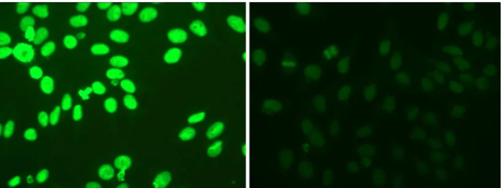
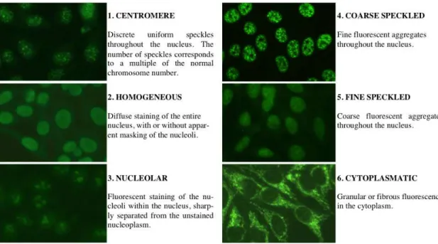
The specialists usually perform a three-step analysis. First, the slide is validated by checking the presence of at least one fluorescence mitotic cell. Second, the in-tensity of fluorescence signal is evaluated according to three levels: negative (i.e. absence of fluorescence), intermediate or positive. Finally, the cells of the interme-diate and positive slides (Figure 1) are classified on the basis of the pattern of the fluorescence signal, which in turn reveals the auto-antibody type. According to lit-erature, the different staining patterns can be classified into six main groups, namely centromere, homogeneous, nucleolar, coarse speckled, fine speckledandcytoplasmatic (Figure 2).
Figure 1: HEp-2 IIF images with positive (left) and intermediate (right) fluorescence intensity.
The accurate classification of the staining patterns is very important for dif-ferential diagnosis, since different patterns are associated with different types of autoimmune diseases. Nevertheless, in the standard practice this process suffers from intrinsic limitations related to the visual evaluation performed by human sub-jects. The analysis of large volume of images is a tedious and time-consuming task and requires highly trained and specialized personnel. Moreover, human evaluation for this type of screening is affected by very high inter laboratory variability (up to 24%, as reported in [2, 3]). This has tremendous impact on the reliability and reproducibility of the obtained results.
Computer-Aided Diagnosis (CAD) systems may overcome these limitations and effectively support the decision of the specialists. In particular, the automation of the staining pattern classification process may considerably reduce the time and effort required by the analysis and, at the same time, improve its repeatability. This would make IIF analysis easier, faster and more reliable.
Figure 2: HEp-2 staining patterns that are considered relevant to diagnostic pur-poses.
Triggered by the growing demand for reliable CAD systems, recent research has proposed solutions for all the major steps of IIF analysis, including methods for (i) the automated segmentation of the HEp-2 cells [4, 5, 6], (ii) the recognition of the mitotic cells in the slides [7,8], (iii) the quantification of fluorescence intensity [9] and (iv) the automated classification of the staining patterns [10,11,12,13,14,15,16]. In particular, most of the recent efforts are focused on the latter task and the proposed classification schemes span the entire spectrum of machine learning (e.g., learning vector quantization [10], decision tree induction algorithms [11,12], support vector machines [15], random forests [16], self-organizing maps [14] and multi-expert systems [13]). The image attributes used to characterize the fluorescent patterns include several types of descriptors, with special focus on morphological and textural features [17, 18].
In spite of the recent extensive research, the accurate classification of the stain-ing patterns still remains a challenge. Moreover, the comparison of the solutions presented in the literature is extremely difficult because they are based on different datasets and different experimental protocols. Conversely, the recent availability of a public dataset of HEp-2 cell images that bounds the researchers to a standardized experimental procedure enables the direct comparability of different approaches [19]. In this paper we describe a new technique for the automated characterization of the staining patterns in HEp-2 IIF images. Our contribution is twofold:
• we propose a set of features to characterize cell images that are highly discrim-inative with respect to their fluorescence patterns. Such feature set is obtained through a detailed analysis of single image attributes, as well as of their integra-tion, and of the selection of the most relevant feature variables. In particular, we investigated image attributes derived from morphological, global and local texture analysis. For each of these categories, we first performed experiments
with different formulations of features to evaluate their individual accuracy. Then, we combined attributes of different categories showing that the aggrega-tion of descriptors of different nature provides a more comprehensive soluaggrega-tion to characterize the HEp-2 fluorescence patterns;
• we propose a Subclass Discriminant Analysis (SDA, [20]) based strategy to remap the cell representations into a novel feature space that provides a better separation of the classes aimed at simultaneously improving the intra-class similarities and inter-class dissimilarities and, thus, at making the classification task easier and more accurate.
A preliminary version of this technique was presented in [21], where we first analysed the use of SDA to approach the staining pattern classification problem, using textural descriptors based on Gray-Level Co-occurrence Matrices (GLCM) and Discrete Cosine Transform (DCT). Here we present a deeper insight into the problem aimed at obtaining a better characterization of the staining patterns and a larger set of experiments supporting our findings.
The rest of the paper is organized as follows. After providing a full characteri-zation of the HEp-2 image dataset in Section 2, in Section 3 we present the main steps of our proposed solution. In Section 4 we describe the experimental protocol and in Section 5 we show and discuss our experimental results. Finally, Section 6 concludes the paper.
2
MATERIALS
The samples used in our experiments were obtained from the MIVIA HEp-2, an annotated database of Indirect Immunofluorescence (IIF) images that is publicly available at [19]. The database was firstly adopted and described in [7] and later used in the 2012 HEp-2 Cells Classification Contest [3]. It contains 28 images of different patients (one image per patient), which were obtained with the following protocol. Each image was acquired with a fluorescence microscope coupled with a 50W mercury vapour lamp and a digital camera having a CCD with square pixels of size 6.45 µm. The microscope observed, with a 40-fold magnification, a slide of HEp-2 substrate prepared with a fixed dilution of 1:80, as recommended in [22]. The size of the IIF images is 1388x1038 pixels and their color bit depth is 24.
Specialists manually segmented and annotated each cell in the IIF images. All the segmentations were reviewed by medical doctors specialized in immunology, which also provided information related to fluorescence intensity, mitotic phase and staining pattern of the cells. Thus, the database provides for each image its fluo-rescence intensity (intermediate or positive) and, for each object in an image, (i) its seed point and bounding box, (ii) a binary mask describing its region of interest (ROI), (iii) the object type (cell, mitotic cell or artifact due to the slide’s preparation process) and, if the object is a non-mitotic cell, (iv) the label of its staining pattern, i.e. one of the six classes reported in Figure2.
The dataset used for training and testing our method contains all and only the normal cells (i.e., neither artifacts nor mitotic cells) of the 28 IIF images included
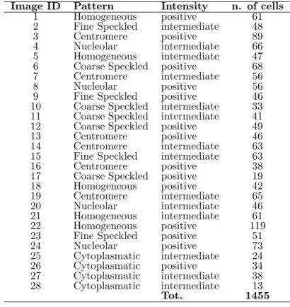
in the MIVIA HEp-2 database. A full characterization of this dataset is reported in Table1.
Table 1: HEp-2 cell dataset characterization, grouped by image ID. Image ID Pattern Intensity n. of cells
1 Homogeneous positive 61 2 Fine Speckled intermediate 48
3 Centromere positive 89
4 Nucleolar intermediate 66 5 Homogeneous intermediate 47 6 Coarse Speckled positive 68 7 Centromere intermediate 56
8 Nucleolar positive 56
9 Fine Speckled positive 46 10 Coarse Speckled intermediate 33 11 Coarse Speckled intermediate 41 12 Coarse Speckled positive 49 13 Centromere positive 46 14 Centromere intermediate 63 15 Fine Speckled intermediate 63 16 Centromere positive 38 17 Coarse Speckled positive 19 18 Homogeneous positive 42 19 Centromere intermediate 65 20 Nucleolar intermediate 46 21 Homogeneous intermediate 61 22 Homogeneous positive 119 23 Fine Speckled positive 51
24 Nucleolar positive 73 25 Cytoplasmatic intermediate 24 26 Cytoplasmatic positive 34 27 Cytoplasmatic intermediate 38 28 Cytoplasmatic intermediate 13 Tot. 1455
3
METHOD
In the recent literature several formulations of image descriptors have been ap-plied to the automated classification of HEp-2 staining patterns. These descriptors are derived from either morphological or textural analysis. However, the relevance of these different types of attributes and their mutual contribution are still open issues.
In several works it has been found that the integration of information of different nature provides a substantial improvement of the classification accuracy [17, 18]. Furthermore, the combination of local and global descriptors has been claimed to generate a more robust mechanism of texture representation [23,24].
Based on these considerations, in our work we performed a detailed analysis of different formulations of morphological, global and local texture characteristics and we investigated, through their integration at different levels, their reciprocal impact on the classification problem.
The outline of the proposed staining pattern classification algorithm is the fol-lowing. For each cell: (i) we normalise its image and (ii) we extract different feature vectors, one for each considered attribute type. When combining different attributes
to characterize a cell image, the corresponding feature vectors are concatenated. Then, for each individual attribute or concatenation of attributes, we select its most relevant feature variables and apply SDA to remap the cell representation into a novel feature space that provides a better class separation. Finally, we train a clas-sifier on a sample set and apply it to a separate test set of samples.
3.1
Image normalisation
Size and intensity normalisation of the samples is a necessary preprocessing step. In fact, small differences in the dimensions of the cell images are normal, and these differences are completely uncorrelated with their staining pattern. On the other hand, there are considerable variations of fluorescence intensity between intermedi-ate and positive samples, and, in a smaller scale, even within cells of the same image (see Figure 1). Reducing such variability helps to decrease the noise in the classi-fication process and avoids as well the necessity of training two separate classifiers for intermediate and positive samples.
In our work, all the cell images were resized to 128x128 pixels. As for the intensity, since the images are produced by green fluorescence, the samples were first converted to grayscale by taking into account only the green channel. Then, intensity normalisation was obtained by linearly remapping all the intensities so that the bottom 1% and the top 1% of all pixel values are saturated at, respectively, the lowest and highest intensities.
3.2
Feature Extraction
In the following, we will use interchangeably the terms “feature set” and “attribute” to refer to the elements used to characterize a cell image according to a specific technique.
As already explained, we took into consideration different image attributes be-longing to three main categories:
1. morphological features, focusing on shape attributes of the fluorescent signal of the cells or of specific regions within the cells;
2. global texture descriptors, which summarize the overall appearance or general distribution of the gray-levels in the cell image;
3. local texture descriptors, which summarize the isolated contribution of small regions or pixel neighbourhoods.
For each of these categories, several approaches have been described in the lit-erature. However, performing an exhaustive analysis of all of them is extremely difficult and out of the scope of this work. Here we focused on the ones that, based on preliminary experiments that we do not report for the sake of brevity, appear to be the most promising for HEp-2 cell characterization. The list of these attributes can be seen in Table 2.
Table 2: Image attributes considered in this work.
Image Attributes size
Morphological Features MORPH 43
Global Texture Features
Gray-Level Co-occurrence Matrices [25,26,27] GLCM 44 Edge Orientation Histograms [28] EOH 80 Rotation-Invariant Gabor features [29] RIGF 32 Modified Zernike moments [30] ZERN 55
Local Texture Features
Rotation-Invariant Uniform Local Binary Patterns [31] LBPriu2
42 Completed Local Binary Patterns [32] CLBP 42 Co-occurrence of adjacent LBPs [33] CoALBP 3072 Rotation-invariant Co-occurrence of adjacent LBPs [34] RIC-LBP 408
3.2.1 Morphological features (MORPH)
Several morphological features have been used to characterize the cell images. The first feature derives from the following consideration. As it is shown in Figure 2, for all the staining patterns except the cytoplasmatic, the fluorescence signal is localized into the nucleus of the cell. Therefore, in these cases, the cell ROI is round or elliptical. On the contrary, the shape of cytoplasmatic patterns is generally more irregular. These differences can be summarized by the ROI circularity, defined asArea/P erimeter2.
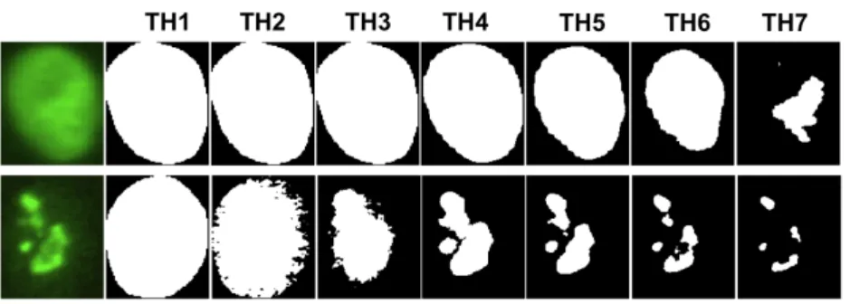
Figure 3: Examples of binary masks obtained from seven progressive thresholding levels (TH1-TH7) applied to images of cells with homogeneous (top) and nucleolar (bottom) staining patterns.
Other morphological measurements are extracted from the binarization of the cell image at increasing intensity thresholds. For each of these thresholds a dif-ferent binary mask is obtained, which isolates the structuring elements of the cell pattern at that specific intensity level. As it can be seen in Figure 3, the shape changes of these masks show a very characteristic behaviour for distinct staining patterns. Therefore, the concatenation of morphological parameters measured at the increasing thresholding levels appears to be effective in characterizing the HEp-2 cell patterns [17].
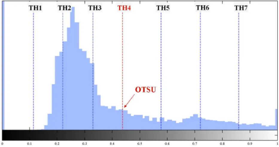
As for the binarization, we used seven progressive thresholds. A first reference value (TH4, in Figure4) is obtained applying the Otsu’s method [35] to the intensity histogram of the cell. The two intervals of the intensity histogram defined by TH4 are further divided intro three equal segments to obtain the other six thresholds, namelyTH1-3andTH5-7for, respectively, the lower and upper parts of the intensity
distribution (see Figure 4).
Figure 4: The seven progressive thresholds computed from a cell intensity histogram. For each binary mask, we then extracted the following morphological properties: 1. proportion of the ROI area covered by foreground pixels;
2. number of connected regions of the foreground;
3. proportion of the connected regions of the foreground which have circular shape (i.e. with circularity >= 0.8);
4. average area of the foreground’s connected regions divided by the total area of the cell ROI;
5. average circularity of the connected regions of the foreground;
6. average solidity of the foreground, where the solidity of each connected region is computed as the percentage of the pixels in the convex hull that also belong to that region.
All the measurements (i.e. the circularity of the ROI, and the six properties ex-tracted at the seven thresholding levels) are finally concatenated, obtaining a de-scriptor of size 43.
Some of the aforementioned properties can be more discriminative for some classes and less for others. For example, features 1 and 4 provide the same val-ues when the foreground contains only one connected region (e.g. the homogeneous pattern in the first row of Figure3) and very different ones in other cases (e.g. the nucleolar pattern in the second row of Figure 3). However, as we will show in the following, the application of a Feature Selection process helps to discard the less relevant variables.
3.2.2 Global textural features (GTF)
Gray-Level Co-occurrence Matrices (GLCM)Several types of global texture descriptors can be computed from Gray-Level Co-occurrence Matrices. These ma-trices report the distribution of co-occurring values between neighbouring pixels
according to different distances and directions [25]. More specifically, each GLCM element (i, j)d,θ contains the probability for a pair of pixels located at a distance d
and direction θ to have gray levels i and j, respectively. In our work, we first com-puted four GLCMs for a fixed unitarian d and a varying θ = 0o,45o,90o,135o after
grouping intensity values into 16 levels. The use of 4 different directions makes the method less sensitive to image rotations. Then, we extracted from each GLCM a to-tal of 22 statistical measures, whose full characterization can be found in [25,26,27]. Finally, we computed the meanM and the range valueR(i.e. maximum-minimum) over the 4 GLCMs for each of these measures, obtaining a total of 44 GLCM features.
Modified Zernike moments (ZERN) Zernike radial polynomials can serve as basis functions to extract image moments, capable of describing the shape and textural characteristics of an object. However, they are strongly affected by changes in scale and position of the objects in the image. An effective descriptor overcoming this limitations and invariant to rotation, translation and scaling, has been presented in [30]. Its invariance properties are obtained computing modified Zernike moments on the normalised power spectrum of the image. In our case, for each cell we extracted a descriptor of 55 elements.
Edge Orientation Histograms (EOH) The general idea of Edge Orientation Histograms (EOH, [28]), as the name suggests, is to represent an image by a his-togram obtained from the predominant gradient orientations of its edge pixels. More specifically, EOH applies a Canny operator to obtain contour pixels from the image, and then it constructs a histogram of directions, counting for each bin the number of contour pixels whose gradient falls within its specific orientation interval. In our work, we computed a 80-dimensional EOH feature vector for each cell image.
Rotation-Invariant Gabor features (RIGF) Gabor filters are widely used for edge detection and texture analysis. Although not rotation invariant, Gabor features can be modified to gain this property by computing their Discrete Fourier Transform (DFT). In this way, the circular shift caused in the Gabor feature vector by an image rotation is converted into a phase shift in the Fourier domain. This phase shift does not affect the magnitude of the DFT coefficients which, therefore, can be used as a rotation-independent representation of textural data. In our work we used the formulation of RIGF proposed in [29], obtaining for each cell a feature vector of dimension 32.
3.2.3 Local textural features (LTF)
In the context of local textural features, one of the most used descriptors is based on local binary patterns (LBPs) [36]. This approach has been found to be very promising also for the characterization of HEp-2 fluorescence patterns [17, 34].
The basic idea behind this descriptor is to represent the texture of the image as a histogram of LBPs,i.e. binary patterns representing the intensity relations between a pixel and its neighbours. For each image pixel, an LBP is obtained by binarizing its neighbouring region using the intensity of the pixel as threshold, and then by converting the resulting binary pattern to a decimal number. Finally, a histogram is generated by taking into account the occurrences of all the LBPs in the image. This is a very simple yet powerful textural descriptor, whose main advantage is the invariance to changes of illumination over the image.
Recent literature reports different descriptors that are supposed to extend and improve the descriptive capabilities of classical LBPs. In our work, we considered the following major formulations.
Rotation-Invariant Uniform Local Binary Patterns (LBPriu2
) A binary pattern is called uniform if it contains not more than two bitwise transitions from 0 to 1 or vice versa when the bit pattern is transversed circularly. Uniform patterns were found to be predominant with respect to other patterns for texture description. Therefore, in [31] they are used to produce compact rotation-invariant LBP feature vectors. In our work we concatenated three histograms with different scales of LBP neighbourhood, as suggested in [31], obtaining a feature vector of dimension 42.
Completed Local Binary Patterns (CLBP) The classical formulation of LBP uses the intensity of the center pixel as threshold for its neighbours. Hence, only the sign of the difference between the center and the neighbour gray values is relevant. The key idea of Completed Local Binary Patterns (CLBP [32]) is to represent each neighbourhood by its center pixel and a local difference sign-magnitude transform (LDSMT) that computes both the sign and the magnitude of the difference between the central pixel and its neighbours. Using the same scale and neighbourhood of LBPriu2, we obtained a 42-dimensional CLBP feature vector.
Co-occurrence of Adjacent LBPs (CoALBP)The original expression of LBPs lacks structural information among different binary patterns. In order to provide them, [33] introduced a novel formulation which measures the co-occurrence among multiple LBPs (and in particular, among adjacent LBPs). This formulation provides a high-dimensional feature vector that has been found to provide a better texture characterization compared to previous LBPs. Concatenating three CoALBP his-tograms with the parameters suggested in [34], the resulting feature vector has size 3072.
Rotation-Invariant Co-occurrence of Adjacent LBPs (RIC-LBP)The CoALBP features can vary significantly depending on the orientation of the target object. In order to cope with this problem, [34] extends the concept of rotation equivalence class ofLBPriu2 to the CoALBPs. This is achieved by attaching a rotation invariant
label to each LBP pair, so that all CoALBPs corresponding to different rotations of the same LBPs have the same value. For each cell image, we extracted and concate-nated three RIC-LBP histograms as suggested by [34], obtaining a feature vector of dimension 408.
3.3
Classification based on Subclass Discriminant Analysis
The categorization of the cell staining patterns is a multiclass classification problem. Our classifier is based on Subclass Discriminant Analysis (SDA), an algorithm that has been recently proposed in [20].
SDA belongs to the family of Discriminant analysis (DA) algorithms, which have been used for dimensionality reduction and feature extraction in many applications. Given a set of samples X = (x1, x2, . . . , xn), where each xi is a vector in ℜD and
has an associated class label ∈ [1, C], DA algorithms compute a mapping of X
to a subspace in ℜd, with d≪D, where the data can be more easily separated
V = (v1, v2, . . . , vd), with vi ∈ ℜD, which, in most DA algorithms, is found by
maximizing the so-called Fisher-Rao’s criterion: J(V) = VTAV |VTBV| (1)
where A and B are symmetric and positive-defined matrices, so that they define a metric. The solution to this problem is given by the generalized eigenvalue decom-position:
AV =BVΛ (2)
where Λ is the diagonal matrix of eigenvalues corresponding to the column-vectors of V.
Linear Discriminant Analysis (LDA) is probably the most well-known DA al-gorithm. It assumes that the C classes the data belong to are homoscedastic, i.e. that their underlying distributions are Gaussian with common variance and different means. In equation (1), LDA uses A = SB, the between-class scatter matrix, and
B =SW, the within-class scatter matrix, which are defined as follows:
SB = C X i=1 (µi−µ)(µi−µ)T (3) SW = 1 n C X i=1 ni X j=1 (xij −µi)(xij −µi)T (4)
wheren is the number of the samples in X, ni the number of samples in class i, µi
is the sample mean for classi, µis the global mean and xij is the jth sample of class
i.
The mapping provided by LDA maximizes the between-class variance and mini-mizes the within-class variance in any particular data set. In other words, it guaran-tees maximal class separability of the training samples and, possibly, optimizes the accuracy in later classification. The main drawback of LDA is that the dimension of the reduced space is bounded by the rank ofSB, which is in turn equal or lower
thanC−1. This means that each sample in the original space is represented by at mostC−1 features. As a consequence, LDA works well for problems that are linear in the origin space, i.e. those for which C−1 features are sufficient to discriminate C classes, but fails to provide optimal subspaces for inherently non-linear structures in data.
To cope with this problem, several extensions of LDA have been introduced in literature [37] and SDA is one of the most effective. The main idea of SDA is to approximate the underlying distribution of each class using a mixture of Gaussians. This is achieved by dividing the classes into a set of subclasses, capable of describing for each class the variance of the data in a more subtle way. Therefore, the main problem to be solved in SDA is to find the optimal number of subclasses for each class.
Once the number of subclasses is known, the transformation matrix V is found by assigning to A in equation (1) the between-subclass scatter matrix defined as:
SB= C−1 X i=1 Hi X j=1 C X k=i+1 Hk X l=1 pijpkl(µij −µkl)(µij −µkl)T (5)
where Hi is the number of subclasses of class i, µij and pij are the mean and prior
probability of the jth subclass of class i, respectively. The priors are estimated as
pij = nij/n, where nij is the number of samples in the jth subclass of class i. With
this formulation of SB, equation (1) works towards the contemporary
maximiza-tion of the distance between the class means and of the one between the means of subclasses of the same class. The objective is, again, to maximize the classification accuracy in the reduced space.
In order to select the optimal number of subclasses, two different methods are proposed in [20] . The first is based on a stability criterion described in [38]. However, as pointed out in [39], the minimization of the metric used in this criterion is not guaranteed when data have a Gaussian homoscedastic subclass structure (and probably even for heteroscedastic). The second selection criterion is based on a leave-one-object test. In practice, a leave-one-out cross validation is applied for each subdivision, and the optimal subdivision is the one maximizing the recognition rate. The problem with this strategy is its very high computational costs, especially with large datasets and high number of classes as in our case. Therefore, in our work we use a slightly different formulation of this criterion, which is based on a stratified 5-fold cross validation of the training set and on the accuracies obtained with a k-Nearest Neighbour (k-NN) classifier.
Our implementation differs from the original SDA formulation for two other details. The first concerns the clustering method. In [20] data are assigned to sub-classes by first sorting the class samples with a Nearest-Neighbour based algorithm and then by dividing the obtained list into a set of equal-sized clusters. However, this method does not allow to model effectively the non-linearity present in the data, as in the case under analysis of HEp-2 staining patterns. Therefore, we used theK-means algorithm, which partitions the samples intoK clusters by minimizing iteratively the sum, over all clusters, of the within-cluster sums of sample-to-cluster-centroid distances.
The second difference is that, instead of increasing at each iteration the number of subclasses of all groups of the same amount, we first choose a maximal number of subclasses for each class, based heuristically on the number of samples per class. Then, all the possible permutations of class subdivisions are tested, halting the subdivision process of a specific class r if the minimal number of samples in any of its current Hr clusters drops below a predefined threshold. In order to reduce
the computational burden, the clusters created for each class and each number of subclasses are computed only once and cached for further use.
Once the optimal number of subclasses have been found and the feature vectors of the samples have been obtained by projecting them on the sub-space defined by SDA, the classification is performed with k-NN. A value of 8 for k has been heuristically found to provide good classification results.
3.4
Feature Selection
Feature selection (FS) is a data preprocessing step that is frequently applied in machine learning. FS extracts the subset of features used to describe the data that improves the classification accuracy. The main purposes of FS are two. First, it reduces the dimensionality of the input data, removing irrelevant information and improving their comprehension by telling which are the most important features and how they are correlated. Second, it improves the chances of avoiding overfitting, whose probability increases with the dimension of the feature space.
In our work, a reduction of the dimensionality of the feature space is already pro-vided by SDA. However, decreasing the initial number of parameters representing the data in order to include only the features that are the most relevant for the con-sidered task improves the separability of the samples in the reduced space computed by SDA and, hence, the classification accuracy (as we will show in Section 5).
We applied a robust feature selection method based on the minimum-Redundancy-Maximum-Relevance (mRMR) algorithm, whose better performance over the con-ventional top-ranking methods has been widely demonstrated in literature [40]. mRMR sorts the features that are most relevant for the characterization of the clas-sification variable, pointing at the contemporaneous minimization of their mutual similarity and maximization of their correlation with the classification label.
However, mRMR provides a mere ranking of the features with no information on the size of the optimal feature set. Therefore, heuristically, we looked for this optimal size by iteratively increasing the number of candidates in the feature set until the global optimum is found. The candidates are selected in order of relevance and, given the computational burden of the classification algorithm, at each itera-tion their number is increased by a factor 10. The initial number of candidates is chosen according to the following consideration. The rank of matrixSB and,
there-fore, the dimensionality d of the reduced subspace obtained with SDA, is given by min(H −1, rank(SX)), where H is the total number of subclasses, SX is the
ma-trix concatenating the representative vectors of the samples in the training set and rank(SX) is equal (or minor) to the number of features characterizing each sample.
Since the data in our problem present high non-linearities, we set as reasonable lower bound ford the value 40.
4
EXPERIMENTAL PROTOCOL
All experiments shown in this paper were run on the HEp-2 cell dataset described in Section 2using the following protocol.
The first experiment applies the leave-one-out technique over all the 28 IIF im-ages composing the dataset. For each image, an instance of the classifier is trained with the cells of the remaining 27 images and then used to classify the cells of the image left out. The classification evaluates each cell individually, without using information on the other cells belonging to the same image. The classification ac-curacy is evaluated (i) on acell-level basis, in terms of percentage of cells correctly classified for each class over all the 28 leave-one-out runs, and (ii) on animage-level basis, in terms of percentage of images correctly classified, using as the predicted
image label the class most frequently assigned to its cells. In both cases, the ac-curacy is obtained by adding the classification counts of the 28 leave-one-out runs (i.e. the number of cells of classi assigned to classj are evaluated by summing the corresponding numbers in each run, and then percentages are computed), and not by averaging the percentages relative to each run.
The leave-one-out method over the images ensures a complete separability and independence of training and test set and it is the experimental protocol that maxi-mizes the number of independent samples (i.e. cells belonging to different patients) used for training. Therefore, it is particularly suited to the HEp-2 cell dataset, that is characterized by a very low number of independent samples per class. Moreover, the execution of several training/test runs with different images allows to assess the robustness and generalization capabilities of the classifier.
A second additional experiment is performed by dividing the images into two sep-arate training and test setsin exactly the same way as it was done in the2012 HEp-2 Cells Classification Contest [3]. The classifier is trained with the cells included in the training set, which contains only 14 of the images of the entire dataset, and the performance of the classifier is assessed on the test set (i.e. the cells belonging to the remaining 14 images). As for the previous experiment, cell-level and image-level accuracies are computed.
5
RESULTS AND DISCUSSION
Our experiments were aimed at answering the following research questions:
• how do the different attributes described in Section3.2contribute to the classi-fication of the HEp-2 staining patterns and how can these individual attributes be combined to improve the classification accuracy? (Section5.1)
• how does SDA strategy cope with the high within-class variance that is typical of HEp-2 staining patterns? (Section5.2)
5.1
Assessing the classification accuracy
For clarity, we briefly recall the main idea behind our feature extraction approach. Morphological, global and local textural descriptors have been found to be the most suitable features for characterizing HEp-2 fluorescence patterns. However, the rel-evance of each of this kind of attributes and their mutual contribution is still an open issue. In this work we postulate that the integration of information of differ-ent nature improves the capabilities of a classifier of recognizing differdiffer-ent staining patterns. To this end, we defined a set of morphological features and we identified different textural descriptors that appeared promising for the task considered.
In the first tests, we computed the classification accuracy (on a cell-level ba-sis) obtained with each individual feature set described in Section 3.2, using the leave-one-out experiment described in Section 4. Then we analysed the accuracies obtained with different groups of attributes.
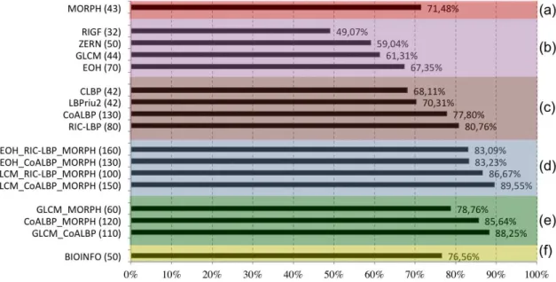
The experimental results are summarized in Figure 5, where we report for dif-ferent feature sets the classification accuracy and (within parentheses) the number of optimal features selected by the FS algorithm.
Figure 5: Cell-level accuracy obtained by different sets of features (leave-one-out experiment). The sections of the graph describe the results of: a) morphological features, b) global textural features, c) local textural features, d) best combinations of the three attribute categories, e) sub-groups of attributes of the best solution, f) our previous approach [21].
Figure 5 is divided into sections showing the accuracies of the individual at-tributes (a-c) and of different combinations of them (d-e). For the sake of brevity, we report only those combinations, between all the ones tested, providing the highest accuracies. For comparison, we also report, in section (f), the accuracy obtained by our previous approach to the problem [21] (feature set named BIOINFO). It should be noted that FS was not applied to attributes whose size was close to, or lower than, 40, which is the limit value for our FS process (Section 3.4).
The following initial remarks can be drawn from the results of Figure 5:
• the single attribute providing the highest accuracy was RIC-LBP (80.76%), followed by CoALBP (77.80%) and MORPH (71.48%);
• considering the categories of individual attributes, local textural features (LTF) performed much better than morphological features, which were in turn better than global textural features (GTF);
• in general, groups of feature sets consistently achieved better results than their single components;
• the integration of morphological and both local and global textural features provided the most comprehensive solution to characterize fluorescence pat-terns. That is, the more heterogeneous the information, the better the accu-racies. The best result (89.55%) was obtained by the combination of GLCM,
CoALBP and MORPH. The accuracy obtained by this optimal group was higher than any partial combination of its composing attributes (shown in figure5(e));
• the proposed method outperformed our previous approach to the problem, which obtained a 76.56% accuracy.
These results require a more detailed discussion. First, while LTF are effective in characterizing the cells, as also found in [3], GTF do not perform equally well. In other words, GTF are less capable of capturing the differences between the various staining patterns, differences that, on the contrary, are more suitably described in terms of local variations of the intensity patterns. The relevance of local information is supported by the results obtained by morphological features, which, in a way, en-code local characteristics into the description of the morphological properties of the cells and of the changes of these properties as a function of the intensity thresholds used to compute them.
Second, the combination of global and local texture descriptors consistently gen-erates a more robust mechanism of texture representation (for example, this is shown in Figure 5 by comparing the accuracy of GLCM-CoALBP, 88.25%, with the ac-curacy of the single attributes, 61.31% and 77.80% respectively). This result is consistent with the findings of previous works [23, 24].
Third, the combination of different attributes generates a completely new mech-anism of image representation compared to the one provided by the same attributes considered individually. Thus, the feature sets best performing individually are not necessarily the ones that will give the best performance when combined together. Indeed, the best GTF and LTF attributes (respectively, EOH with 67.35% and RIC-LBP with 80.76%) are not included into the group that obtained the highest accuracy and, for instance, much better accuracies are obtained with groups based on GLCM as GTF and on CoALBP as LTF. This could be explained as follows:
• the integration with other features helps to soften the major limitations of specific attributes (e.g., the dependence from texture rotations of CoALBP);
• Feature Selection contributes to this scenario by selecting a compact set of features that helps to reduce the noise and by strengthening the mutual con-tribution of specific attributes.
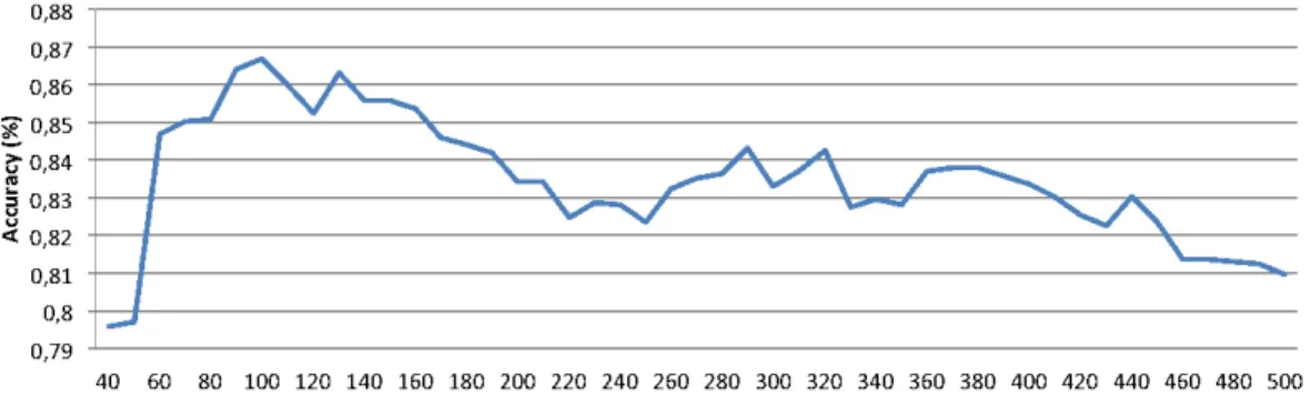
Feature Selection deserves another detailed discussion. As expected, FS always significantly improves the accuracy. As an example, in Figure 6 we show, for the group GLCM-RIC-LBP-MORPH, the behaviour of the accuracy against the number of features used by the classifier. As it can be seen, the accuracy reaches a global maximum for 100 features improving of more than 5% the accuracy obtained with all the 495 feature variables. Another interesting result is that the total accuracy around the optimal set size is rather stable (i.e. less than 2% in the range between 60 and 160), indicating that the performance of the proposed approach is not strictly tied to a precise identification of the optimal size. For other attributes and attribute groups, including the optimal GLCM-CoALBP-MORPH group, we obtained similar results that we omit for brevity. We simply underline the fact that with very large
feature sets (e.g. those including CoALBP), the performance drop between the optimal set and the full feature set is significantly higher than the one shown in the example of Figure 6. As a matter of facts, in these cases, since the classifiers are based on a number of features largely greater than the number of observations, results with no FS are likely to be affected by overfitting. We believe that these results highlight as well the capabilities of FS to prevent this problem.
Figure 6: Cell classification accuracy vs. size of the feature set (features set GLCM-RIC-LBP-MORPH,leave-one-out experiment).
The analysis of the features surviving the FS pruning can provide some insights into the cell characteristics that are more relevant for the classification of the staining patterns. In general, in all groups all types of features are present, with a slight preference for local texture descriptors. If we consider, as an example, the optimal combination GLCM-CoALBP-MORPH, we have that, of the 150 features selected, 16 come from GLCM (out of a total of 44), 106 from CoALBP (3072) and the remaining 28 from MORPH (43). This is another evidence of the fact that features with different nature are effectively combined to provide a substantial improvement of the accuracy.
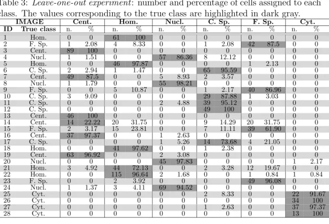
Concluding this section, we present the detailed results of the optimal solution found for this first experiment (GLCM-CoALBP-MORPH). In Table 3 we show for each of the 28 IIF images its true class and the number and the percentage of the image cells labelled with each of the six staining patterns. Table 4 shows on the left the confusion matrix and the total accuracy of cell classification (89.55%) and, on the right, the image-level confusion matrix and the total accuracy of image classification (96.43%).
5.2
Discriminative capabilities of SDA
Another interesting subject of analysis is the discriminative capability of our SDA-based classification approach. For the discussion of this issue, we will also make use of the results obtained with the second experiment described in Section 4, which is based on two separate training and test sets. For the sake of conciseness, we do not report the detailed results of this experiment, which basically confirmed the main findings of theleave-one-out experiment:
Table 3: Leave-one-out experiment: number and percentage of cells assigned to each class. The values corresponding to the true class are highlighted in dark gray.
IMAGE Cent. Hom. Nucl. C. Sp. F. Sp. Cyt.
ID True class n. % n. % n. % n. % n. % n. % 1 Hom. 0 0 61 100 0 0 0 0 0 0 0 0 2 F. Sp. 1 2.08 4 8.33 0 0 1 2.08 42 87.5 0 0 3 Cent. 89 100 0 0 0 0 0 0 0 0 0 0 4 Nucl. 1 1.51 0 0 57 86.36 8 12.12 0 0 0 0 5 Hom. 0 0 46 97.87 0 0 0 0 1 2.13 0 0 6 C. Sp. 2 2.94 1 1.47 0 0 65 95.59 0 0 0 0 7 Cent. 49 87.5 0 0 5 8.93 2 3.57 0 0 0 0 8 Nucl. 1 1.79 0 0 55 98.21 0 0 0 0 0 0 9 F. Sp. 0 0 5 10.87 0 0 1 2.17 40 86.96 0 0 10 C. Sp. 3 9.09 0 0 0 0 29 87.88 1 3.03 0 0 11 C. Sp. 0 0 0 0 2 4.88 39 95.12 0 0 0 0 12 C. Sp. 0 0 0 0 0 0 49 100 0 0 0 0 13 Cent. 46 100 0 0 0 0 0 0 0 0 0 0 14 Cent. 14 22.22 20 31.75 0 0 9 14.29 20 31.75 0 0 15 F. Sp. 2 3.17 15 23.81 0 0 7 11.11 39 61.90 0 0 16 Cent. 37 97.37 0 0 1 2.63 0 0 0 0 0 0 17 C. Sp. 0 0 0 0 1 5.26 14 73.68 4 21.05 0 0 18 Hom. 0 0 41 97.62 0 0 1 2.38 0 0 0 0 19 Cent. 63 96.92 0 0 2 3.08 0 0 0 0 0 0 20 Nucl. 0 0 0 0 45 97.83 0 0 0 0 1 2.17 21 Hom. 3 4.92 44 72.13 0 0 2 3.28 12 19.67 0 0 22 Hom. 0 0 115 96.64 2 1.68 0 0 1 0.84 1 0.84 23 F. Sp. 0 0 2 3.92 0 0 0 0 49 96.08 0 0 24 Nucl. 1 1.37 3 4.11 69 94.52 0 0 0 0 0 0 25 Cyt. 0 0 0 0 0 0 2 8.33 0 0 22 91.67 26 Cyt. 0 0 0 0 0 0 0 0 0 0 34 100 27 Cyt. 0 0 0 0 0 0 1 2.63 0 0 37 97.37 28 Cyt. 0 0 0 0 0 0 0 0 0 0 13 100
Table 4: Leave-one-out experiment: confusion matrices (%).
CELL CLASSIFICATION IMAGE CLASSIFICATION
class Cent. Hom. Nucl. C. Sp. F. Sp. Cyt. Cent. Hom. Nucl. C. Sp. F. Sp. Cyt. Cent. 83.47 5.60 2.24 3.08 5.60 0 83.33 16.67 0 0 0 0 Hom. 0.91 93.03 0.61 0.91 4.24 0.30 0 100 0 0 0 0 Nucl. 1.25 1.24 93.78 3.32 0 0.41 0 0 100 0 0 0 C. Sp. 2.38 0.48 1.43 93.33 2.38 0 0 0 0 100 0 0 F. Sp. 1.44 12.5 0 4.33 81.73 0 0 0 0 0 100 0 Cyt. 0 0 0 2.75 0 97.25 0 0 0 0 0 100
Total accuracy = 89.55% Total accuracy = 96.43%
• the combination of morphological, global and local textural information guar-antees the highest accuracies;
• the optimal solution is provided, again, by the GLCM-CoALBP-MORPH group (with 100 features), although in this experiment other groups perform in a comparable way at both cell and image-level.
• the performance around the optimal set size is, again, rather stable, indicating that the accuracy is not strictly tied to a precise identification of the optimal number of features.
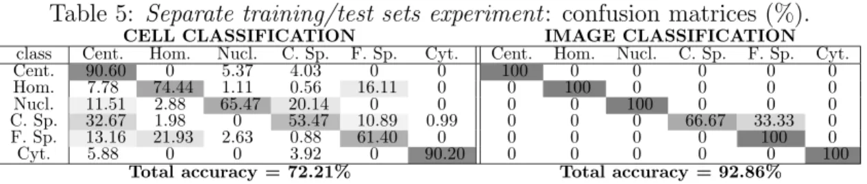
For completeness, we detail the best result achieved in Table 5, where as before we show the confusion matrix and classification accuracy at cell-level (on the left) and at image-level (on the right). As it can be seen, the cell-level accuracy drops drastically from the 89.55% of the first experiment to the current 72.21%, while the accuracy at image level is similar (92.86% vs. 96.43% of the leave-one-out experiment, both corresponding to a single misclassified image).
This difference can be easily explained in terms of the characteristics of the training and test sets. In the second experiment, the availability of only 14 differ-ent images for training, coupled with the high within-class variance presdiffer-ent in the HEp-2 cell patterns, translates into very few independent samples per class. As a consequence, the manifolds of the various staining patterns in the feature space are likely to be under-sampled, thus hampering the SDA capabilities to model them in a suitable manner and, consequently, reducing the cell-level classification accuracy of the whole method. The better performance at image-level can be simply explained analysing in details the results of theleave-one-out experiment (Table 3), where the per class correct accuracies are most of the times greater than 85%. Therefore, even if more cells are misclassified in the second experiment, the ones maintaining the correct label are still sufficient, in most of the cases, to assign the correct image label.
Table 5: Separate training/test sets experiment: confusion matrices (%).
CELL CLASSIFICATION IMAGE CLASSIFICATION
class Cent. Hom. Nucl. C. Sp. F. Sp. Cyt. Cent. Hom. Nucl. C. Sp. F. Sp. Cyt. Cent. 90.60 0 5.37 4.03 0 0 100 0 0 0 0 0 Hom. 7.78 74.44 1.11 0.56 16.11 0 0 100 0 0 0 0 Nucl. 11.51 2.88 65.47 20.14 0 0 0 0 100 0 0 0 C. Sp. 32.67 1.98 0 53.47 10.89 0.99 0 0 0 66.67 33.33 0 F. Sp. 13.16 21.93 2.63 0.88 61.40 0 0 0 0 0 100 0 Cyt. 5.88 0 0 3.92 0 90.20 0 0 0 0 0 100
Total accuracy = 72.21% Total accuracy = 92.86%
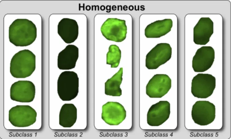
The protocol of the second experiment let us also inspect in more details the strategy used by SDA in dividing class samples into subclasses. In fact, differently from the leave-one-out method, where the optimal class subdivision is likely to vary at each fold, the use of a single training set translates into a single optimal partition of subclasses. If we consider as an example the best solution shown in Table 5, the number of subclasses is two for nucleolar and centromere classes, three for cytoplasmatic class, four for coarse and fine speckled and five for homogeneous class.
For nucleolar and centromere classes, SDA performs a straightforward subdivi-sion between cells with intermediate and positive fluorescence intensity. For other classes (e.g. the homogeneous pattern) the subdivision splits the cells in a more subtle way, grouping cells of similar appearance in the same subclass (Figure 7), which is obviously of major help for the classification process.
Finally, in order to further assess the discriminative capabilities of our SDA-based approach, we compared our method with Support Vector Machines (SVM), a state-of-the-art classifier that is widely recognized for its classification performance by computer scientists and machine learning researchers. For the classification, we used SVM with a radial basis kernel, optimizing its parameters by means of a grid search as suggested in [41]. Then, we applied the two-step FS process described in [15]: we first chose for each single/composite attribute a candidate feature set of size 200 with mRMR, or directly the whole feature set if its size was lower than 200, and then we reduced it to an optimal size applying a Sequential Forward Selection scheme (more details in [15]).
We repeated with SVM all the tests in the two experiments obtaining, on average, classification accuracies lower than SDA-based approach by about 10% in the
leave-Figure 7: Sample images from the five homogeneous subclasses obtained in the optimal solution shown in Table5.
one-out experiment and about 3% in the separate training-test set experiment. Concluding, we think that all these results further support our hypothesis that SDA, being particularly suited to deal with the high within-class heterogeneity of HEp-2 cell images, is a promising approach for staining pattern classification.
6
CONCLUSIONS AND FUTURE WORKS
In this paper we described an automated solution for HEp-2 staining pattern clas-sification in IIF images based on Subclass Discriminant Analysis approach.
The main findings of our work are two. First, after investigating the contribu-tion of several types of attributes, individually and grouped, we obtained an optimal set of features that combines morphological descriptors with global and local tex-tural analysis based on, respectively, GLCM and CoALBP features. With this set of attributes we achieved a classification accuracy close to 90%, showing that the integration of information of different nature provides an effective representation of the fluorescence patterns. Furthermore, the classification accuracy was stable in a neighborhood of the optimal set size, indicating a good robustness of the proposed approach. Second, we verified that the proposed SDA-based strategy can effectively cope with the high within-class variance of HEp-2 samples and, coupled with a Fea-ture Selection process, can provide a compact set of image attributes that is highly discriminative and effective for the classification task.
As future works, we are planning to implement a complete solution tackling all the steps of an automated IIF analysis, including the quantification of the staining intensity, the cell segmentation and the recognition of the mitotic cells. Further improvements of the SDA-based solution will be also investigated, e.g. by experi-menting different types of classifiers other thank-NN.
References
[1] K. Egerer, D. Roggenbuck, R. Hiemann, M. Weyer, T. Buettner, B. Radau, R. Krause, B. Lehmann, E. Feist, G. Burmester, Automated evaluation of au-toantibodies on human epithelial-2 cells as an approach to standardize cell-based immunofluorescence tests., Arthritis Res Ther 12 (2) (2010) R40.
[2] N. Bizzaro, R. Tozzoli, E. Tonutti, A. Piazza, F. Manoni, A. Ghirardello, D. Bassetti, D. Villalta, M. Pradella, P. Rizzotti, Variability between meth-ods to determine ana, anti-dsdna and anti-ena autoantibodies: a collaborative study with the biomedical industry, Journal of Immunological Methods 219 (12) (1998) 99 – 107.
[3] P. Foggia, G. Percannella, P. Soda, M. Vento, Benchmarking HEp-2 Cells Clas-sification Methods, Medical Imaging, IEEE Transactions on, (2013).
[4] Y.-L. Huang, Y.-L. Jao, T.-Y. Hsieh, C.-W. Chung, Adaptive automatic seg-mentation of hep-2 cells in indirect immunofluorescence images, in: Proceedings of the 2008 IEEE International Conference on Sensor Networks, Ubiquitous, and Trustworthy Computing (sutc 2008), SUTC ’08, 2008, pp. 418–422.
[5] C. Creemers, K. Guerti, S. Geerts, K. Van Cotthem, A. Ledda, V. Spruyt, Hep-2 cell pattern segmentation for the support of autoimmune disease diagnosis, in: Proceedings of the 4th International Symposium on Applied Sciences in Biomedical and Communication Technologies, ISABEL ’11, 2011, pp. 28:1– 28:5.
[6] G. Percannella, P. Soda, M. Vento, A classification-based approach to segment hep-2 cells, in: Computer-Based Medical Systems (CBMS), 2012 25th Interna-tional Symposium on, 2012, pp. 1–5.
[7] P. Foggia, G. Percannella, P. Soda, M. Vento, Early experiences in mitotic cells recognition on hep-2 slides, in: Computer-Based Medical Systems (CBMS), 2010 IEEE 23rd International Symposium on, 2010, pp. 38–43.
[8] G. Percannella, P. Soda, M. Vento, Mitotic hep-2 cells recognition under class skew, in: Image Analysis and Processing ICIAP 2011, Vol. 6979 of Lecture Notes in Computer Science, Springer Berlin Heidelberg, 2011, pp. 353–362. [9] P. Soda, G. Iannello, M. Vento, A multiple expert system for classifying
flu-orescent intensity in antinuclear autoantibodies analysis, Pattern Anal. Appl. 12 (3) (2009) 215–226.
[10] T.-Y. Hsieh, Y.-C. Huang, C.-W. Chung, Y.-L. Huang, Hep-2 cell classification in indirect immunofluorescence image, in: Proceedings of the 7th international conference on Information, communications and signal processing, ICICS’09, 2009, pp. 211–214.
[11] P. Perner, H. Perner, B. Mller, Mining knowledge for hep-2 cell image classifi-cation, Artificial Intelligence in Medicine 26 (2002) 161–173.
[12] U. Sack, S. Knoechner, H. Warschkau, U. Pigla, F. Emmrich, M. Kamprad, Computer-assisted classification of hep-2 immunofluorescence patterns in au-toimmune diagnostics, Autoimmunity Reviews 2 (5) (2003) 298 – 304.
[13] P. Soda, G. Iannello, A hybrid multi-expert systems for hep-2 staining pattern classification, in: Proceedings of the 14th International Conference on Image Analysis and Processing, 2007, pp. 685–690.
[14] Y.-C. Huang, T.-Y. Hsieh, C.-Y. Chang, W.-T. Cheng, Y.-C. Lin, Y.-L. Huang, Hep-2 cell images classification based on textural and statistic features using self-organizing map, in: Proceedings of the 4th Asian conference on Intelligent Information and Database Systems - Volume Part II, ACIIDS’12, 2012, pp. 529–538.
[15] S. Di Cataldo, A. Bottino, E. Ficarra, E. Macii, Applying textural features to the classification of hep-2 cell patterns in iif images, in: Proceedings of the 21st International Conference on Pattern Recognition, ICPR 2012, 2012.
[16] P. Strandmark, J. Ulen, F. Kahl, Hep-2 staining pattern classification, in: Pat-tern Recognition (ICPR), 2012 21st InPat-ternational Conference on, Nov., pp. 33–36.
[17] I. Theodorakopoulos, D. Kastaniotis, G. Economou, S. Fotopoulos, Hep-2 cells classification via fusion of morphological and textural features., in: IEEE 12th International Conference on Bioinformatics and Bioengineering (BIBE), 2012, pp. 689–694.
[18] G. Thibault, J. Angulo, Efficient statistical/morphological cell texture charac-terization and classification, in: Pattern Recognition (ICPR), 2012 21st Inter-national Conference on, 2012, pp. 2440 –2443.
[19] http://mivia.unisa.it/datasets/biomedical-image-datasets/hep2-image-dataset
(Last accessed: march 2013).
[20] M. Zhu, A. M. Martinez, Subclass discriminant analysis, IEEE Trans. Pattern Anal. Mach. Intell. 28 (8).
[21] I. Islam, S. Di Cataldo, A. Bottino, E. Ficarra, E. Macii, Classification of hep-2 staining patterns in immunofluorescence images - comparison of support vector machines and subclass discriminant analysis strategies, in: Proceedings of the International Conference on Bioinformatics Models, Methods and Algorithms, 2013, pp. 1–9.
[22] R. Tozzoli, N. Bizzaro, E. Tonutti, D. Villalta, D. Bassetti, F. Manoni, A. Pi-azza, M. Pradella, P. Rizzotti, Guidelines for the laboratory use of autoantibody tests in the diagnosis and monitoring of autoimmune rheumatic diseases., Am J Clin Pathol 117 (2) (2002) 316–24.
[23] Y. Xu, S. B. Huang, H. Ji, Integrating local feature and global statistics for texture analysis, in: Image Processing (ICIP), 2009 16th IEEE International Conference on, 2009, pp. 1377 –1380.
[24] J. A. Montoya-Zegarra, J. Beeck, N. Leite, R. Torres, A. Falc˜ao, Combining global with local texture information for image retrieval applications, in: Pro-ceedings of the 2008 Tenth IEEE International Symposium on Multimedia, ISM ’08, 2008, pp. 148–153.
[25] R. M. Haralick, K. Shanmugam, I. Dinstein, Textural Features for Image Clas-sification, Systems, Man and Cybernetics, IEEE Transactions on SMC-3 (6) (1973) 610–621.
[26] L. kiat Soh, C. Tsatsoulis, Texture analysis of sar sea ice imagery using gray level co-occurrence matrices, IEEE TRANSACTIONS ON GEOSCIENCE AND REMOTE SENSING (1999) 780–795.
[27] D. Clausi, An analysis of co-occurrence texture statistics as a function of grey level quantization, Can. J. Remote Sensing 1 (28) (2002) 45–62.
[28] A. Pinheiro, Image descriptors based on the edge orientation, in: Semantic Me-dia Adaptation and Personalization, 2009. SMAP ’09. 4th International Work-shop on, 2009, pp. 73–78.
[29] F. Bianconi, A. Fern´andez, A. Mancini, Assessment of rotation-invariant tex-ture classification through Gabor filters and discrete Fourier transform, in: Proceedings of the 20th International Congress on Graphical Engineering (XX INGEGRAF), Valencia, Spain, 2008.
[30] D.-G. Sim, H.-K. Kim, R.-H. Park, Invariant texture retrieval using modified Zernike moments, Image and Vision Computing 22 (4) (2004) 331–342.
[31] T. Ojala, M. Pietik¨ainen, T. M¨aenp¨a¨a, Multiresolution gray-scale and rotation invariant texture classification with local binary patterns, IEEE Trans. Pattern Anal. Mach. Intell. 24 (7) (2002) 971–987.
[32] Z. Guo, D. Zhang, D. Zhang, A completed modeling of local binary pattern operator for texture classification, Image Processing, IEEE Transactions on 19 (6) (June) 1657–1663.
[33] R. Nosaka, Y. Ohkawa, K. Fukui, Feature extraction based on co-occurrence of adjacent local binary patterns., in: Lecture Notes in Computer Science, Vol. 7088, Springer, 2011, pp. 82–91.
[34] R. Nosaka, C. H. Suryanto, K. Fukui, Rotation invariant co-occurrence among adjacent lbps, in: Proceedings of the ACCV2012 Workshop LBP2012, 2012, pp. 1–11.
[35] N. Otsu, A threshold selection method from gray-level histograms, IEEE Trans-actions on Systems, Man and Cybernetics 9 (1) (1979) 62–66.
[36] T. Ojala, M. Pietik¨ainen, D. Harwood, A comparative study of texture measures with classification based on featured distributions, Pattern Recognition 29 (1) (1996) 51–59.
[37] N. Boulgouris, K. N. Plataniotis, E. Micheli-Tzanakou, Discriminant analysis for dimensionality reduction: An overview of recent developments, Biometrics: Theory, Methods, and Applications, Wiley.
[38] A. M. Martinez, M. Zhu, Where are linear feature extraction methods applica-ble?, IEEE Transactions on Pattern Analysis and Machine Intelligence 27 (12) (2005) 1934–1944.
[39] N. Gkalelis, V. Mezaris, I. Kompatsiaris, Mixture subclass discriminant analy-sis, IEEE Signal Process. Lett. 18 (5) (2011) 319–322.
[40] H. Peng, F. Long, C. Ding, Feature selection based on mutual information: criteria of max-dependency, max-relevance, and min-redundancy, IEEE Trans-actions on Pattern Analysis and Machine Intelligence 27 (2005) 1226–1238. [41] C. C. Chang, C. J. Lin, LIBSVM: A library for support vector machines, ACM