O
pen
A
rchive
T
OULOUSE
A
rchive
O
uverte (
OATAO
)
OATAO is an open access repository that collects the work of Toulouse researchers and
makes it freely available over the web where possible.
This is an author-deposited version published in :
http://oatao.univ-toulouse.fr/
Eprints ID : 12719
To link to this article
: DOI :10.1109/TNNLS.2013.2286696
URL :
http://dx.doi.org/10.1109/TNNLS.2013.2286696
To cite this version
: Laporte, Léa and Flamary, Rémi and Canu,
Stéphane and Déjean, Sébastien and Mothe, Josiane
Non-convex
Regularizations for Feature Selection in Ranking with Sparse SVM
.
(2014) IEEE Transactions on Neural Networks, vol. 25 (n° 6). pp.
1118-1130. ISSN 1045-9227
Any correspondance concerning this service should be sent to the repository
administrator:
[email protected]
Nonconvex Regularizations for Feature Selection in
Ranking With Sparse SVM
Léa Laporte, Rémi Flamary, Stéphane Canu, Sébastien Déjean, and Josiane Mothe Abstract— Feature selection in learning to rank has recently
emerged as a crucial issue. Whereas several preprocessing approaches have been proposed, only a few have focused on integrating feature selection into the learning process. In this paper, we propose a general framework for feature selection in learning to rank using support vector machines with a sparse regularization term. We investigate both classical convex regularizations, such asℓ1or weightedℓ1, and nonconvex
regu-larization terms, such as log penalty, minimax concave penalty, or
ℓp pseudo-norm with p<1. Two algorithms are proposed: the
first, an accelerated proximal approach for solving the convex problems, and, the second, a reweighted ℓ1 scheme to address
nonconvex regularizations. We conduct intensive experiments on nine datasets from Letor 3.0 and Letor 4.0 corpora. Numerical results show that the use of nonconvex regularizations we propose leads to more sparsity in the resulting models while preserving the prediction performance. The number of features is decreased by up to a factor of 6 compared to theℓ1regularization. In addition, the software is publicly available on the web.1
Index Terms— Feature selection, forward–backward splitting algorithms, learning to rank, nonconvex regularizations, regularized support vector machines, sparsity.
I. INTRODUCTION
L
EARNING to rank is a crucial issue in the field of information retrieval (IR). The main goal of learning to rank is to learn automatically ranking functions using a machine learning algorithm, in order to optimize the ranking of documents or web pages. Several algorithms have been proposed during the past decade [1], which can combine a very large number of features to learn ranking functions.Whereas the number of features that can be used by algo-rithms has increased, the issue of feature selection in learning to rank has emerged, for two main reasons.
Manuscript received December 17, 2012; accepted October 1, 2013. Date of publication November 13, 2013; date of current version May 15, 2014. This work was supported in part by CALMIP under Grant 2012-32, in part by the FR3424 Research Federation FREMIT, and in part by the Conseil Général of Midi-Pyrénées under Project 10009108.
L. Laporte is with the Institut de Recherche en Informatique de Toulouse CNRS UMR 5505, Université de Toulouse, Toulouse Cedex 9 31062, France and is also with Nomao SA, Toulouse 31500, France
R. Flamary is with the Laboratoire Lagrange, Université de Nice-Sophia, Nice 06108, France (e-mail: [email protected]).
S. Canu is with LITIS, INSA de Rouen and Normandie Université, Saint-Etienne-du-Rouvray 76800, France (e-mail: [email protected]).
S. Déjean is with the Institut de Mathématiques de Toulouse CNRS UMR 5219, Université de Toulouse, Toulouse Cedex 9 31062, France
J. Mothe is with the Institut de Recherche en Informatique de Toulouse CNRS UMR 5505, ESPE Académie de Toulouse, Université de Toulouse, Toulouse Cedex 9 31062, France
First, as more and more features are incorporated into algorithms, not only do the models become more difficult to understand but they also potentially have to deal with more and more noisy or irrelevant features. As feature selection is well known in machine learning to deal with noisy and irrelevant features, it is seen as a quite natural way to solve this problem in learning to rank.
Second, the amount of training data used in learning to rank is substantial. As a consequence, learning a ranking function using algorithms is generally costly and can be time consuming. Reducing the number of features, and thus the dimensionality of the problem, is a promising way to handle the issue of high computational cost.
Recent works have focused on the development of feature selection methods dedicated to learning to rank, which can be either preprocessing steps such as filter [2]–[4] and wrapper approaches [4]–[7], or integrated to the learning algorithm, such as embedded approaches [8]–[10]. In the latter case, the learning algorithm is called a sparse algorithm. In this paper, we consider an embedded approach for feature selection in learning to rank. We propose a general framework for feature selection in learning to rank using support vector machines (SVMs) and a regularization term to induce sparsity. We investigate both convex regularizaions such asℓ1[11] and nonconvex regularizations such as minimax concave penalty (MCP) [12], log or ℓp, p < 1 [13]. To the best of our knowledge, this is the first work that investigates the use of nonconvex penalties for feature selection in learning to rank. We first propose an accelerated forward–backward split-ting (FBS) algorithm to solve the ℓ1-regularized problem. Then, we propose a reweighted ℓ1 algorithm to handle the nonconvex penalties, which benefits from the first algorithm. We conduct intensive experiments on the Letor 3.0 and 4.0 corpora. Our convex algorithm leads to a similar per-formance as the state-of-the-art methods. We show that the second algorithm, which uses nonconvex regularizations, is a very competitive feature selection method since it provides as good results as convex approaches but is much more per-forming in terms of sparsity. Indeed, it provides similar values of evaluation measures while using half as many features on average.
This paper is organized as follows. Section II presents the state of the art for learning to rank algorithms, feature selection methods, sparse SVM, and FBS approaches. We formulate the optimization problem in Section III. Section IV intro-duces the algorithms used to solve the optimization problems. We fully describe the datasets used and the experimental protocol in Section V. In Section VI, we first analyze the
ability of our approach to induce sparsity into models. We then evaluate the performance of our framework in terms of mean average precision (MAP) and normalized discounted cumulative gain (NDCG)@10. We compare these results with those obtained with two recent embedded feature selection methods.
II. RELATEDWORKS
This paper focuses on feature selection in learning to rank. We begin this section by presenting existing learning-to-rank algorithms. We provide an overview of feature selection methods dedicated to learning to rank and introduce feature selection using sparse regularized SVMs.
A. Learning-to-Rank Algorithms
The learning-to-rank process consists of a training phase and a prediction phase. In IR, the training data are com-posed of query–document pairs represented by feature vectors. A relevance judgment between the query and the document is given as ground truth. The purpose of the training phase is to learn a model that provides the optimum ranking of documents according to their relevance to the query. The ability of the model to correctly rank documents for new queries is then evaluated during the prediction phase, on test data. The following is a short overview of learning-to-rank approaches and algorithms. A more complete introduction to learning to rank for IR can be found in [1].
Three approaches, called pointwise, pairwise, and listwise, have been proposed to solve the learning-to-rank problem. In the pointwise approach, each instance is a vector of features
xi, which represents a query–document pair. The ground truth can be either a relevance scores∈R or a class of relevance (such as “not relevant,” “quite relevant,” “highly relevant”). When dealing with a relevance score, learning to rank is seen as a regression problem. Some algorithms such as subset ranking [14] have been proposed to solve it. When dealing with classes of relevance, learning to rank is considered as a classification problem or as an ordinal regression problem, depending on whether there is an ordinal relation between the classes of relevance. Some algorithms based on SVMs [15] or on boosting [16] deal with the classification problem. Crammer and Singer [17] proposed an algorithm for ordinal regression. In the pairwise approach, also referred to as preference learning [18], each instance is a pair of feature vectors(xi,xj)for a given queryq. The ground truth is given as a preference y ∈ {−1,1} between the two documents. For a given couple (xi,xj), if xi is preferred to xj, we note
xi ≻q xj and then y is set to 1. On the contrary, if xj is preferred to xi, we note xj ≻q xi and then y is set to −1. It is thus a classification problem. Many algorithms have been developed to deal with this problem, such as RankNet [19] based on neural networks, RankBoost [20] based on boosting, or RankSVM-Primal [21] and RankSVM-Struct [22] based on SVMs. Finally, the listwise approach considers the whole ranked list of documents as the instance of the algorithm. Most works have focused on the proposal of new specific loss
TABLE I
CLASSIFICATION OFFEATURESELECTIONALGORITHMS FORLEARNING TORANKINTOFILTER, WRAPPER,ANDEMBEDDEDCATEGORIES
functions, based on the optimization of an IR metric or on permutations count to solve this kind of problem [23], [24].
These approaches have been shown to be both efficient and effective to learn functions that ensure high ranking performance in terms of IR measures. Nevertheless, they may be suboptimal for use in real life with large-scale data. Ranking functions deal with a very large amount of features, which raises three critical issues. First, as features may take time to compute, preprocessing steps such as the creation of training data may become time consuming. Second, due to the high dimensionality of training data, algorithms may not be scalable or they may take too much time for computation. Finally, there may be a significant amount of redundant or irrelevant features used by models, which can lead to suboptimal ranking performance. Thus, how to reduce the number of features to be used by algorithms has emerged as a crucial issue. Nevertheless, only a few attempts have been made to solve this problem. In the following section, we propose an overview of the existing feature selection methods in classification and learning-to-rank.
B. Feature Selection Methods in Learning to Rank
In classification, there are three kinds of feature selec-tion methods, called filter, wrapper, and embedded. In filter methods, a subset of features is selected as a preprocessing step, independently of the predictor used for learning. In wrapper methods, the machine learning algorithm is used as a black box to score subsets of features according to their predictive power. The subset with the highest score is then chosen. Finally, in embedded methods, feature selection is performed within the training phase and incorporated to the algorithm. Embedded methods are generally specific to a given machine learning algorithm. A broad introduction to feature selection for classification is presented in [25]. Feature selection methods for learning to rank have been developed in a similar way as in classification. We propose an overview of feature selection methods for learning to rank in the following section, and classify them into filter, wrapper, and embedded categories in Table I.
To the best of our knowledge, the first proposal of a feature selection method dedicated to learning to rank is the work of Geng et al. [2]. Their method is called the greedy search
algorithm for feature selection (GAS) and belongs to the filter approaches. For each feature, they first define its importance score: they rank instances according to feature values and
evaluate the performance of the ranking list with a measure such as MAP or NDCG. This evaluation measure is then used as the importance score for the feature. For each pair of fea-tures, they also define a similarity score, which is the value of the Kendall’sτ between the rankings induced by the features
of the pair. Kendall’sτ is defined as follows: ifxandyare two
features andDthe number of document pairs, thenτ (x,y)=
(#{(ds,dt)∈D|dt ≻x ds anddt≻y ds}/#{(ds,dt)∈D}), where
dt ≻x ds indicates that the document dt is ranked above the documentds according to the value of featurex. An optimiza-tion problem is then formulated to select features by simulta-neously maximizing the total importance score and minimizing the total similarity score. This optimization problem is solved by a greedy search algorithm. They show that the GAS algorithm can significantly improve the performance in terms of MAP or NDCG while reducing the number of features.
Huaet al. [3] later proposed a two-phase feature selection
strategy. In a first step, they define the similarity between features in the same way as in the GAS algorithm. Features are then clustered into groups according to their similarity, by using a k-means approach. The number of clusters to
be used is chosen according to a quality measure defined by the authors. In a second step, they propose to select a single representative feature from each cluster to learn the model. They use two delegation strategies for this purpose: a filter one based on evaluation measure (BEM) and a wrapper one implied by the learning-to-rank method used (ILTR). The BEM delegation method selects the feature whose ranking has the best evaluation score. The ILTR delegation method learns a linear model using a learning-to-rank algorithm. For each cluster, the representative feature is then the one with the highest weight in the ranking function. They show that BEM and ILTR techniques can significantly improve the performance in terms of NDCG@10 compared to models with no feature selection.
Some other works have focused on the development of wrapper approaches for feature selection on learning to rank. Panet al.[5] proposed a method using boosted regression
trees. In a method similar to [2], they define an importance score for each feature and a similarity score for each pair of features. The importance score is the relative importance score as defined in [26] for regression-boosted trees. The similarity score is defined by the Kendall’s τ between the vectors of values for the features of the pairs. The authors investigate three optimization problems: 1) to maximize the importance score; 2) to minimize the similarity score; and 3) to simultaneously maximize the importance score and minimize the similarity score. These optimization problems are solved by a greedy approach. Experiments show that better results are obtained when only using the importance score than when using the importance and similarity scores. Moreover, they point out that a 30-features model achieves similar performance in terms of NDCG@5 than the complete model with 419 features. In a second approach, they propose a randomized feature selection with a feature-importance-based backward elimination. In practice, they create subsets of features, then iteratively train boosted trees, and remove a per-centage of features according to their NDCG@5 performance.
The experimental results show that these methods achieve comparable performance to that of the complete model by using only 30 features.
Yuet al.[4] proposed two effective feature selection
meth-ods for ranking based on relief algorithms [27]. Relief algo-rithms are iterative methods that update the feature weights at each iteration based on their importance. The authors propose RankWrapper, a wrapper approach for training data with rela-tive orderings, and RankFilter, a filter approach from training data with multilevel relevance classes. They also define new updating rules for the weights for each algorithm. Experiments on synthetic and benchmark datasets show that their method outperforms the GAS algorithm and can be used with large-scale datasets.
Dang and Croft [6] proposed a feature selection technique based on the wrapper approach defined in [28]. They use a best-first search procedure to create subsets of features. For each subset, they train a model with a ranking algorithm. The output is defined as a new feature. A new feature vector is then created with the output of each subset and contains fewer features than the initial dataset. Models are trained using this vector with four well-known learning-to-rank algorithms: RankNet, RankBoost, AdaRank, and coordinate ascent. Their experiments on the Letor datasets show that they produce comparable performance in terms of NDCG@5 by using the smaller feature vector.
Finally, Pahikkala et al. [7] proposed an algorithm called
greedy RankRLS, which is a wrapper approach based on the existing RankRLS algorithm. Subsets of features are created on which a leave-query-out cross-validation is performed by using the RankRLS algorithm. Results on the Letor 4.0 distribution show that the performance in terms of MAP and NDCG@10 are comparable to state-of-the-art algorithms with all the features.
Recently, embedded methods have been proposed to deal with the problem of feature selection. These approaches introduce a sparse regularization term in the formulation of the optimization problem. Although sparse regularizations are widely used in classification to deal with feature selection, only a few attempts have been made to propose sparse-regularized learning-to-rank methods. Sun et al. [8]
imple-mented a sparse algorithm called RSRank to directly optimize the NDCG. They propose a framework to reduce ranking to importance-weighted pairwise classification. To achieve sparsity, they introduce a ℓ1-regularization term and solve the optimization problem using truncated gradient descent. Experiments on Ohsumed and TD2003 datasets show that only about a third of features remained after the selection. Moreover, the performance of the learned model is comparable to or significantly better than the baselines, depending on the dataset and the measure used.
A more recent work [9] proposes a primal-dual algorithm for learning-to-rank called FenchelRank. The authors formu-late the sparse learning to rank problem as an SVM problem with anℓ1-regularization term. They use the properties of the Fenchel duality to solve the optimization problem. Basically, FenchelRank is an iterative algorithm that works in three steps. At each iteration, it first checks whether the stopping criterion
is satisfied. If not, the algorithm then greedily chooses a feature to update according to its value. Finally, it updates the weights of the ranking model. Experiments were conducted on several datasets from the Letor 3.0 and Letor 4.0 collections. The authors show that FenchelRank leads to a good sparsity with sparsity ratios from 0.1875 to 0.5. It also provides comparable or significantly better results in terms of MAP and NDCG than state-of-art algorithms and RSRank. Finally, Lai et al.
[10] recently proposed a new embedded algorithm for feature selection based on sparse SVMs. This algorithm solves a joint convex optimization problem in order to learn ranking functions while automatically selecting the best features. They use a Nesterov approach to ensure fast convergence. They show that FSMRank can learn efficiently ranking models that outperform the GAS algorithm.
In classification, a large panel of embedded methods has been developed to learn sparse models with SVMs. As far as we know, FenchelRank and FSMRank are the only ones to use sparse SVMs for feature selection in learning-to-rank. Sparse SVMs could widely and efficiently be adapted in this purpose. In this paper, we focus on SVM methods with a sparse-regularized term for which we propose a short overview in the following section.
C. Learning as Regularized Empirical Loss Minimization
The structural risk minimization is a useful and widely used induction principle in machine learning. It states that the learning task can be defined as the following optimization problem (for a given positive constantC)
min w,b C n ! i=1 L(x⊤i w+b,yi)+(w). (1) The loss function L(·,·) is the data-fitting term measuring the discrepancy for all training examples{xi,yi}between the predicted value f(x) = x⊤w+b and the observed value y. The second term(·)is a penalty providing regularization and
controlling generalization ability through model complexity. Note that the training examples may also be expressed as a matrix X = [x1, . . . ,xn]⊤ ∈ Rn×d and a vector y =
[y1, . . . ,yn]⊤∈Rn containing the output objective values. Many choices are possible for the loss functionL(., .)such
as the hinge loss, the squared hinge loss, or the logistic loss for classification problems or the ℓ2-loss or the Hubert loss for a regression problem. Similarly, the regularization term
(·) can be the usual ℓ2-regularization, also known as ridge regularization (2(w)= ||w||22), or theℓ1-regularization term, also known as lasso with 1(w) = ||w||1 = "j|wj|. The latter has been proposed in the context of linear regression by Tibishirani [11] in order to promote automated feature selection.
D. Feature Selection via Penalization
When dealing with feature selection, the structural mini-mization principle still holds. In this case, the relevant penalty from the statistical point of view is theℓ0regularization term. It is defined as 0(w) = kwk0 = "dj=11{wd
j=1>0}, i.e.,
the number of nonzero components in vector w. But the
minimization of such functional suffers severe drawbacks for optimization: it is nonconvex, noncontinuous, or nondifferen-tiable (in zero).
A way to tackle these issues is to relax theℓ0constraint by replacing0(w) by another penalty. A popular choice is the
ℓ1-regularization term. It has several advantages such as being convex and thus providing tractable optimization problems.
However, while theℓ1lasso penalty alleviates the optimiza-tion issues raised by theℓ0penalty, it brings some statistical concerns since it has been shown to be, in certain cases, inconsistent for variable selection and biased [29]. A simple way to obtain nice statistical properties while preserving the computational efficiency of the ℓ1 minimization is to use a weighted lasso penalty by assigning different weights to each coefficient. This leads to the weightedℓ1 regularization
β(w) = "dj=1βj|wj|, where the βj > 0 are the data-dependent weights of each variable. The next step is proposing a suitable choice for these weights.
For regression problems, [29] proposed to useβj =1/wLSj , wherewLSj is the nonregularized least-squares estimator. This
approach cannot be applied in our framework because the com-putation of the unpenalized solution is intractable. Instead, we propose to derive these weights from a nonconvex relaxation theℓ0pseudo-norm of the form
(w)=
d
!
j=1
g(|wj|) (2) where g(·) are nonconvex functions. Indeed, when it is well
chosen, the nonconvex nature of functiongwill provide good
statistical properties such as unbiasedness and oracle inequal-ities [12], while the use of a weighted ℓ1 implementation scheme will ensure nice computational behavior. This can be obtained because the associated problem has been shown to be part of a more general optimization framework that can be solved using a simple reweighed ℓ1 scheme with βj =
g′(|w∗
j|), as presented in Section IV-C, whereg′ denotes the derivative ofgandw∗j is a previously computed solution [30].
Among all possible choices forg, we can cite theℓp pseudo-norm with p < 1 proposed by [31] and used more recently
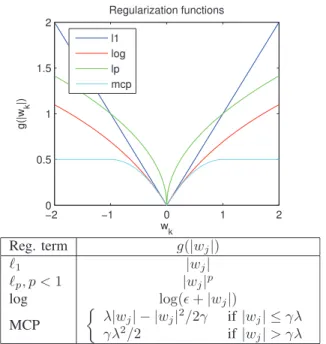
in compressed sensing applications [32]. Another well-known approximation of the ℓ0 penalty is the log penalty that has been introduced in [33] in the context of variable selection. The MCP has been proposed in [12] in order to minimize the bias introduced by classical ℓ1 regularizations. The smoothly clipped absolute deviation is another popular choice. These regularization terms are plotted in Fig. 1, while their definition is recalled in the associated table.
In Section III, we formulate the sparse regularized prob-lem. In Section IV, we propose two algorithms to solve this nondifferentiable problem.
III. PROBLEMSTATEMENT
A. Preference Learning With SVM
We consider a learning-to-rank problem in IR for which the document ranking according to queries is to be optimized.
Fig. 1. Comparison of several nonconvex regularization terms.ǫ=1 and
γ=1 are the parameters, respectively, for the log and MCP regularizations.
LetQbe the total number of queries andDthe total number of
documents in the training dataset T. Then,Q= {qk}k=1,...,Q is the set of all queries, and D= {di}i=1,...,N is the set of all documents. Each (query, document) pair is represented by a vector of featuresφ(qk,di) ∈Rd, where d is the number of features. Let w∈Rd be the vector of weights of the learned model. We also define rk= {(i,j)i,j=1,...,N|di ≻qk dj}as the
subset of all the indices (i,j)i,j=1,...,N for which there is a preference betweendi anddj for the queryqk.
The optimization problem to be solved in pairwise SVM for ranking is defined as in [22] min w∈Rd,ξi,j,k 1 2kwk 2 2+C ! i,j,k ξi,j,k (3) under the constraints
∀(di,dj)∈r1,wT(φ(q1,di)−φ(q1,dj)) >1−ξi,j,1 .. . ∀(di,dj)∈rQ,wT(φ(qQ,di)−φ(qQ,dj)) >1−ξi,j,Q and ∀i,∀j,∀k, ξi,j,k ≥0.
We can reduce this problem to a classification problem. Let Ik = {ik}
i=1,...,Nand((i,.)or(.,i))∈rk) be the subset of indices of
documents that take part of a preference relation for queryqk. We can then define the following vectors:
D = [{i ∈I1}. . .{i ∈IQ}] Q= [1' () *. . .1 card{I1} . . .k' () *. . .k card{Ik} . . .Q. . .Q ' () * card{IQ} ]
where D ∈ R"kQ=1card{Ik}, and Q ∈ R"kQ=1card{Ik}. Then, the
subset P ∈ Rn×n of all preference relations in the training
dataset T is defined as
P = {(s,t)s=1,...,n;t=1,...,n|(D(s),D(t))∈rQ(s)=Q(t)}.
Each feature vector can be written as φ(., .) = xs,s = 1, . . . ,n, and X ∈ Rn×d is the matrix of all xs vectors. The pairwise optimization problem is defined as
min w,ξp 1 2kwk 2 2+C P ! p=1 ξp (4) under the constraints
+
˜
xpw≥1−ξp
ξp≥0 ∀p=1, . . . ,P
where x˜p = xsT − xtT corresponds to a unique pair and
,
X = [˜x1, . . . ,x˜1]⊤ ∈ RP×d is thus the matrix of all prefer-ences pairs. Problem 4 is then equivalent to problem 3 and is written as a classification problem. By using the square hinge loss such asξp=max(0,1− ˜x⊤pw)2, the pairwise optimization problem finally is min w 1 2kwk 2 2+C P ! p=1 max(0,1− ˜x⊤pw)2. (5) The use of the square hinge loss in this context, as proposed in [21], is for differentiability reasons when solving the pairwise problem in the primal.
B. Sparse Regularized SVM for Preferences Ranking
To achieve feature selection in the context of SVM, a common solution is to introduce a sparse regularization term. We propose in the following to consider the Lasso formulation for feature selection, which combinesℓ1-sparsity term and a square loss.
In classification, the Lasso SVM solves the following opti-mization problem: min w kwk1+C n ! i=1 max(0,1−yix⊤i w) 2 . (6)
According to (5) and (6), we directly formulate the pairwise Lasso SVM by replacing theℓ2-term by aℓ1-term, as
min w kwk1+C P ! p=1 max(0,1− ˜x⊤i w)2. (7) The optimization problem for pairwise learning to rank with Lasso SVM is thus reduced to a Lasso classification problem on the matrix of preferences. One critical issue may arise when using this formulation. Indeed, as the ℓ1-norm is not differentiable, this problem might be quite difficult to solve. However, a large number of methods and algorithms have been proposed in classification in order to solve it. Thus, we argue that considering pairwise sparse SVMs is perfectly well suited to select features in learning to rank, for two reasons.
First, contrary to several proposed approaches such as GAS, sparse regularized SVM methods do not require extra developments of similarity and importance measures dedicated
to learning-to-rank. Indeed, the feature selection is only based on the properties of the regularization term, so no additional assumptions are needed. Second, as they follow the SVM framework for classification, methods and algorithms used in classification can easily be adapted and applied to learning-to-rank with a few implementation efforts. In this paper, we propose to use an adaptation of a fast iterative shrinkage tresholding algorithm in order to solve the sparse regularized optimization problem and to proceed to feature selection. We present this algorithm in the following section. We also propose to use nonconvex regularization instead ofℓ1-penalty in order to counter the statistical issues that may arise. We propose a second algorithm in the following section to deal with the nonconvex regularizations.
IV. LEARNINGPREFERENCESWITHSPARSESVM In this section, we discuss the proposed methods for learn-ing preferences with sparse SVM. First, we introduce the FBS algorithm, which is a well-known approach for solving the nondifferentiable weighted-ℓ1 regularized problem. Sec-ond, this algorithm is adapted to the problem of preference learning and its convergence is proved. Finally, we propose a general approach for solving the learning problem with nonconvex regularization terms.
A. Forward–Backward Splitting Algorithm for Feature Selection
FBS algorithms were proposed initially to solve nondiffer-entiable optimization problems such as ℓ1-norm regularized learning problems. A good introduction to this kind of algo-rithm is given in [34]. When minimizing a problem of the form
min
w∈Rd J1(w)+λ(w) (8)
where J1(·) is a differentiable objective function with a
Lipschitz-continuous gradient and (·) is a convex regular-ization term having a closed-form proximity operator, the proximity operator of regularizationµ(·)is defined as
Proxµ(z)=arg min
w
1
2kz−wk 2
2+µ(w). (9) FBS algorithms are iterative methods that compute at each iteration the proximity operator of the regularization term on a gradient descent step with respect to the differentiable function, thus leading to the following update:
wk+1=Proxλ L -wk− 1 L∇J1(w k) . (10) where 1/L is a gradient step and L has to be a
Lip-schitz constant of ∇J1 in order to ensure convergence. Note that one can easily compute the proximity operator of the
ℓ1-regularization, which is of the following form:
Proxλk·k1(w)j =max -0,1− λ |wj| . wj =sign(wj)(|wj| −λ)+ ∀j∈1, . . . ,d. (11)
Algorithm 1Accelerated FBS Algorithm 1:Initializew0
2:Initialize L as a Lipschitz constant of∇J1(·)
3:k =1,z1=w0,t1=1 4:repeat 5: wk←Prox λ L(z k− 1 L∇J1(zk)) 6: tk+1← 1+ √ 1+4(tk)2 2 7: zk+1←wk+/tk−1 tk+1 0 (wk−wk−1) 8: k ←k+1 9:untilConvergence
The weighted ℓ1 regularization has a similar proximity oper-ator Proxλβ(w)j =max -0,1− λβj |wj| . wj =sign(wj)(|wj| −λβj)+ ∀j ∈1, . . . ,d. (12) This algorithm, also known as iterative shrinkage thresholding algorithm (ISTA), has been proposed to solve linear inverse problems withℓ1-regularization, as presented in [35]. In their paper, Beck and Teboulle also address one limitation of this kind of approach: the speed of convergence. Although these algorithms are able to deal with large-scale data, they may converge slowly. Beck and Teboulle proposed to use a multi-step version of the algorithm called fast iterative shrinkage thresholding algorithm (FISTA) which will converge more quickly to the optimal objective value. This algorithm can be seen in Algorithm 1.
B. FBS for Sparse Preference Learning
In this section, we discuss how we adapted the FISTA algorithm to the problem of preference learning withℓ1 and weightedℓ1-regularized SVMs.
First, we note that (7) is a sum of a differential function, the data fitting loss, and a nondifferentiableℓ1-regularization. We then solve the equivalent problem as in (8) with
(w)= ||w||1,λ=1/C, and J1(w)="Pp=1max(0,1− ˜x⊤pw)2. In order to ensure convergence of the algorithm, the cost function J1(w) must have a Lipschitz-continuous gradient.
Then, we just have to prove the following proposition.
Proposition 1: Let J1(w) the square Hinge loss
J1(w)=
P
!
p=1
max(0,1− ˜x⊤pw)2.
Then its gradient
∇J1(w)= −2 P ! p=1 ˜ xpmax(0,1− ˜x⊤pw) is Lipschitz and continuous.
Proof: The squared Hinge loss is gradient-Lipschitz if
there exists a constant L such that
The proof essentially relies on showing that x˜imax(0,1−
˜
x⊤
i w)is Lipschitz itself, i.e., there exists L′∈Rsuch that
k˜ximax(0,1− ˜xi⊤w1)− ˜ximax(0,1− ˜x⊤i w2)k
≤L′kw1−w2k.
Now let us consider different situations. For a given w1and
w2, if 1− ˜xiTw1≤0 and 1− ˜xTi w2≤0, then the left-hand side (LHS) is equal to 0 and any L′ would satisfy the inequality.
If 1− ˜xT
iw1≤0 and 1− ˜xTi w2≥0, then the LHS is lhs= k˜xik2(1− ˜x⊤i w2)
≤ k˜xik2(x˜i⊤w1− ˜x⊤i w2)
≤ k˜xik22kw1−w2k2.
A similar reasoning yields the same bound when 1− ˜xTiw1≥0
and 1− ˜xT
i w1≤0 and 1− ˜xiTw2≥0 and 1− ˜xiTw2≥0. Thus,
˜
ximax(0,1− ˜xi⊤w)is Lipschitz with a constantk˜xik2. Now, we can conclude the proof by stating that ∇wJ is Lipschitz
as it is a sum of Lipschitz function and the related constant is "n
i=1k˜xik22.
We thus have proved than J1(w)has a Lipschitz-continuous
gradient, which ensures the convergence of the algorithm. The gradient of J1(w) is easy to compute and can be used as it in the FISTA algorithm. We thus can use the FISTA algorithm to solve the ℓ1 and weighted-ℓ1-regularized SVM problems. We called this algorithm RankSVM-ℓ1.
C. Algorithm for Nonconvex Regularization
When using a nonconvex regularization term as presented in equation (2), the previous algorithm cannot be used. We propose in this case to adapt a general-purpose framework that has been proposed in [30]. The main idea behind this framework is to cast the regularization term as a difference of two convex functions. Convergence to a stationary point has been proven on this particular class of problems when performing a primal/dual optimization [36].
The approach introduced in [30] can also be seen as a majorization minimization method [37]. Indeed, one can clearly see in Fig. 1 that all of the proposed regularization terms are concave in their positive orthant. This implies that for a fixed pointu0>0
∀u>0, g(u)≤g(u0)+g′(u0)(u−u0).
The algorithm consists in minimizing iteratively the majoration of the cost function. When removing the constant term, the optimization problem for iterationk+1 is
wk+1=arg min
w∈Rd J1(w)+λ
!
i
βj|wj| (13) where βi = g′(|wki|) is computed using the solution at the previous iteration. This approach is extremely interesting in our case, as we can readily use the efficient algorithm proposed for the weighted ℓ1 regularization. Moreover, one can use a warm-starting scheme for initializing the solver at the previous iteration. The resulting algorithm is given as Algorithm 2, and the derivative functionsg′(·)for the nonconvex regularizations are given in Table II.
Algorithm 2Solver for Nonconvex Regularization 1:Initializew0andk=1
2:Initializeβj =1,∀j
3:repeat
4: wk← Minimize majorization (13) using algorithm 1.
5: βj ←g′(|wkj|),∀j
6: k ←k+1
7:untilConvergence
TABLE II
DERIVATIVES OF THENONCONVEXREGULARIZATIONTERMS
V. EXPERIMENTALFRAMEWORK
A set of numerical experiments have been conducted on benchmark datasets to evaluate the performance of the frame-work we proposed. In this section, we provide a full descrip-tion of the datasets and the measures used. We also present the experimental protocol.
A. Datasets
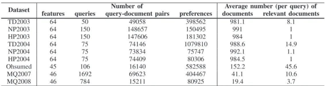
We conduct our experiments on Letor 3.0 and Letor 4.0 collections. These are benchmarks dedicated to learning-to-rank. Letor 3.0 contains seven datasets: Ohsumed, TD2003, TD2004, HP2003, HP2004, NP2003, and NP2004. Letor 4.0 contains two datasets: MQ2007 and MQ2008. Their charac-teristics are summarized in Table III. Each dataset is divided into five folds, in order to perform cross validation. For each fold, we dispose of train, test, and validation sets.
B. Evaluation Measures
We evaluate the ranking performance of our approach using MAP and NDCG. MAP is a standard evaluation measure in information retrieval that works with binary relevance judg-ments: relevant or not relevant. It is based on the computation of the precision at the positionk, which represents the fraction
of relevant documents at the positionk in the ranking list for
a queryq Pq@k =
#relevant documents within thek top documents
k .
The average precision (AP) at the positionk is then defined
for the queryq as
APq=
"k
i=1P@i.1{document i is relevant} #relevant documents for the queryq.
MAP is defined as the average of AP over all the queries MAP= 1 Q Q ! q=1 APq.
Unlike MAP, the NDCG can deal with more than two levels of relevance. Letr(i) be the relevance level of the document
TABLE III
CHARACTERISTICS OFLETOR3.0ANDLETOR4.0 DISTRIBUTIONS
at positioni. Given a queryq, the discounted cumulative gain
at positionk is defined as DCGq@k = k ! i=1 2r(i) −1 log2(i+1).
DCG can take values greater than 1. A normalization term is then introduced to set the values from 0 to 1
NDCGq@k= 1
Zk
DCGq@k where Zk is the maximum value of DCG@k.
We also evaluate the ability of our approach to promote sparsity. To this purpose, we compute the sparsity ratio, which is the fraction of remaining features in the model after selection. For each fold f ∈ 1, . . . ,NT of the dataset T,
where NT is the number of folds, we define the sparsity ratio
SRf as SRf =
#remaining features in the learned model #features of the given dataset . We do not consider features that are zero for all the queries. Thus, the total number of features of a given dataset can be smaller than indicated in Table III. The sparsity ratio of the algorithmAfor a given dataset T is the average of SR over all the folds
SR(A,T)= 1 NT NT ! f=1 SRf. C. Experimental Protocol
For each dataset, we first train the algorithms on the training set with different values of C on a grid. For each fold,
the C value that leads to the best MAP performance on
the validation set is chosen. The model trained with this
C value is used for prediction on the test set. We
com-pute the MAP and the NDCG@10 on the test dataset. We then compare the convex algorithm and the nonconvex algo-rithm with the state-of-the-art methods, namely FenchelRank and FSMRank. We do not compare our method with the GAS algorithm, since it has been proven to be outperformed by the FSMRank algorithm [10]. We run the Windows/MsDos FenchelRank executable provided on the author’s personal web page2 and the MATLAB code of FSMRank provided by the
2scholat.com/~hanjiang. Last visited on 12/09/2012.
authors on demand. We use the same grid as the authors to tune the parameters. Note that, since we use the MAP instead of the NDCG@10 to choose the optimal value of r on the
validation, we obtain different models and results from those in [9] and [10]. Finally, we set γ = 2 for the MCP penalty andǫ =0.1 for the log penalty, which are values commonly
used in the community.
For each experiment, we use the paired one-sided Student test in order to evaluate the significance of our results. A result is significantly better than another if the p-value provided by
the Student test is lower than 5%. Results on performance in terms of sparsity ratio are illustrated by a spider (or radar) plot. Spider plots allow us to easily compare the behavior of several algorithms on several datasets according to a given measure. Each branch of the plot represents a dataset, while each line stands for an algorithm.
VI. RESULTS ANDDISCUSSION
In this section, we compare our convex and nonconvex frameworks with state-of-the-art methods. First, we analyze the performance of the nonconvex framework in terms of sparsity ratio. Second, we show that using nonconvex reg-ularizations leads to similar results both in terms of MAP and NDCG@10. Finally, we evaluate the sparsity ratio and the performance in terms of IR measures to demonstrate that nonconvex regularizations are truly competitive compared to state-of-the-art approaches.
A. Sparsity Ratio
As we stated in the introduction, feature selection is a key issue in learning-to-rank. We aim at providing effective methods that can learn high-quality models while automat-ically selecting a small number of highly informative fea-tures. The main goal of using nonconvex regularizations is to sharply reduce the number of features used in ranking models. In this section, we analyze the sparsity ratio we obtain by using nonconvex penalties and compare them with the two algorithms FenchelRank and FSMRank as well as ourℓ1algorithm.
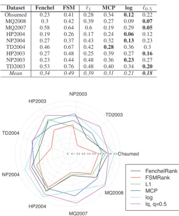
Table IV presents the sparsity ratio obtained with Fenchel-Rank, FSMFenchel-Rank, andℓ1regularization and the three noncon-vex penalties log, MCP, andℓ0.5. We restrict our analysis to this value of p for readability reasons. Fig. 2 presents the
TABLE IV
COMPARISON OFSPARSITYRATIOBETWEENCONVEX ANDNONCONVEX REGULARIZATIONS ANDSTATE-OF-THE-ARTALGORITHMS
Fig. 2. Ratio of removed features for each algorithm and regularization on Letor 3.0 and 4.0 corpora.
features. The larger this measure, the better the algorithm is to induce sparsity into models.
We first observe on both Table IV and Fig. 2 that, on average, methods that use convex penalty are not as sparse as those using nonconvex regularizations. Methods that use the ℓ1 penalty are less sparse. In particular, FSMRank leads to higher sparsity ratios on most of the datasets, which means that the learned models contain many more features than those learned by the other methods. The MCP penalty appears to be the least sparse of the nonconvex penalties. This is not really surprising since the MCP penalty has been initially proposed not as a feature selection approach but as a way to minimize the bias induced byℓ1 regularization.
When considering the average sparsity ratio, the use of log andℓppenalties makes sense. These two nonconvex penalties lead to the smallest sparsity ratio. The learned models select, on average, half the features used by convex regularizations on all datasets. When considering each dataset independently, log andℓp penalties select up to 12 times fewer features than the convex ones. These penalties are then truly performing meth-ods to achieve feature selection. The log penalty is particularly effective for inducing sparsity on HP2003, TD2003, and the MQ datasets. For these latter datasets, it selects from around 6–12 times fewer features than the state-of-the-art algorithms. The log penalty is the most effective for inducing sparsity on Ohsumed, HP2004, and NP2004 datasets. It can frequently
select from one-quarter to one-half fewer features than the convex regularizations. More precisely:
1) on Ohsumed, the log penalty selects from one-half to one-third as many features than convex and MCP penalties;
2) on MQ2008, there were 4–6 times fewer features used by ℓ0.5 than by convex or MCP regularizations, while the log penalty selects 2–3 times fewer features; 3) on MQ2007, the log penalty selects half as many
fea-tures as convex and MCP penalties, while ℓ0.5 selects 10–12 times fewer features that convex regularizations and MCP;
4) on HP2004, the two nonconvex penalties use from one-quarter to one-half as many features as MCP and convex regularizations;
5) on NP2004, the log penalty selects from half to one-third as many features as MCP and convex regulariza-tions;
6) on TD2004 and HP2003, there were 2–3 times fewer features used byℓ0.5than by MCP and convex regular-izations;
7) on TD2003, the nonconvexℓ0.5penalty use half as many features as MCP and convex regularizations.
Nonconvex penalties are thus shown to be very competitive methods when considering the number of selected features. The difference of sparsity ratio observed between the datasets is due to the intrinsic difference between datasets. Ohsumed dataset, Letor 4.0, and Letor 3.0 collections do not use the same features. Although the features are similar for HP, NP, and TD datasets, those are not related to similar retrieval tasks. The number of relevant features may vary from a kind of datasets to another, and so does the relevant features themselves. Nevertheless, we may reasonably expect to select the same features on datasets related to the same tasks. The different performance in terms of sparsity ratio of a given algorithm among the datasets should not be seen as drawback of the method but as the specificity of the dataset.
Removing a large number of features may not be accurate if it leads to a degradation of the prediction quality. In the following section, we compare the performance in terms of IR measures between nonconvex and convex regularizations.
B. Performance in Terms of IR Measures
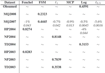
In this section, we compare the prediction of our proposed frameworks to those of the two state-of-the-art algorithms FenchelRank and FSMRank. Table V (respectively, Table VI) indicates the algorithm that leads to the best value of MAP (respectively, NDCG@10). Each algorithm is also compared with the best algorithm by using the unilateral one-sided stu-dent test. If a significant decrease is observed, the percentage of degradation and the p-value are indicated. If no significant
variation is observed, the two algorithms are considered as equivalent and the ∼ symbol is used. When considering MAP and NDCG values, one can notice that some algorithms perform better on some datasets than the others. This is not specific to our methods and had already been observed for learning-to-rank algorithms [1].
TABLE V
COMPARISON OFMAP BETWEEN THEBESTMETHOD ONEACHDATASET ANDOTHERALGORITHMS. BESTMAP IS INBOLD. THE∼SYMBOL INDICATESEQUIVALENCEBETWEENTWOMETHODS. PERCENTAGE OF
DECREASEISPRESENTEDWHENSTATISTICALLYSIGNIFICANT UNDER THE5% THRESHOLD(p-VALUES INITALICS)
TABLE VI
COMPARISON OFNDCG@10 BETWEEN THEBESTMETHOD ONEACH DATASET ANDOTHERALGORITHMS. BESTMAP IS INBOLD. THE∼SYMBOLINDICATESEQUIVALENCEBETWEENTWOMETHODS.
PERCENTAGE OFDECREASEISPRESENTEDWHENSTATISTICALLY SIGNIFICANTUNDER THE5% THRESHOLD(p-VALUES INITALICS)
1) General Results: All the algorithms tend to provide
similar results in terms of both MAP and NDCG@10 on the several datasets. Nevertheless, some differences in terms of performance can be observed among the algorithms, especially on HP2004 and NP2004 datasets on which we notice the largest variations of MAP and NDCG@10. A more detailed study is conducted in order to determine whether these differ-ence are significant.
2) MAP Analysis: We notice that on four datasets, i.e.,
Ohsumed, MQ2008, NP2004, and TD2003, all the algorithms provide similar results than the best algorithm. On the other five datasets, we observe that some convex and nonconvex algorithms can lead to some degradation of the evaluation
measure. We observe small decreases (less than 1%) in half the cases. Limited (between 3% and 4%) and higher (up to 11%) decreases also occurred. A deeper analysis follows.
FSMRank provides the higher value of MAP on the MQ2007 dataset. Our proximal approach with ℓ1 regular-ization is the only one that leads to equivalent results. We observed a very small decrease of the MAP when using FenchelRank (−0.8%) and our reweighted framework with MCP and log penalties (−0.5% and−0.7%, respectively). The use of the ℓpregularization leads to a 3% degradation of the MAP, which is still reasonable.
FenchelRank provides the best MAP results on HP2004; but all the other algorithms and regularizations provide compara-ble results, except the log penalty. The framework using the log regularization leads to a degradation of 11% of the MAP, so the use of this penalty might not be a good choice in term of MAP performance on this particular dataset. When using nonconvex penalties, theℓp or MCP should be preferred on this dataset.
On TD2004 dataset, we observe a significant degradation of the MAP only when considering the MCP regularization. The other nonconvex penalties and the ℓ1 regularization lead to results equivalent to those of the best algorithm. On NP2003 dataset, all the algorithms lead to similar results, except when using theℓp penalty, for which a small variation is observed. Finally, we notice that all the nonconvex penalties provide as good results as ourℓ1algorithm, for which the MAP is the highest. FSMRank is the only one for which a degradation is observed.
All in all, the framework we proposed leads to competitive results in terms of MAP. Theℓ1algorithm is the best on one dataset and provides equivalent results on all other datasets. The MCP regularization leads to the best MAP values on two datasets and is equivalent to the best method on five datasets. The log and ℓp penalties provides results similar to those of the best algorithm on seven datasets.
3) NDCG@10 Analysis: When considering NDCG@10,
we observe that most of the algorithms provide similar results on most of the datasets. The highest NDCG@10 values are obtained by FenchelRank on two datasets, FSMRank on two datasets, our ℓ1 framework on three datasets, and our framework with nonconvex log penalty on two datasets. Nevertheless, all the algorithms provide results similar to those of the best algorithm on seven datasets, including Ohsumed, MQ2008, NP2004, TD2004, HP2003, NP2003, and TD2003. Thus, our framework leads to performance similar to that of the state-of-the-art algorithms and can provide highest NDCG@10 values, although the improvement is not significant.
As we notice for the MAP, FSMRank provides the best val-ues on the MQ2007 dataset. We observe significant decreases for all the others algorithms, although the degradations are small (less than 1% in most cases). On the HP2004 datasets, our framework performs as well as the best algorithm, except for the log penalty. In this last case, we observe a 4% decrease for NDCG@10.
Experiments thus show that our convex and nonconvex frameworks provide similar results as those of the convex
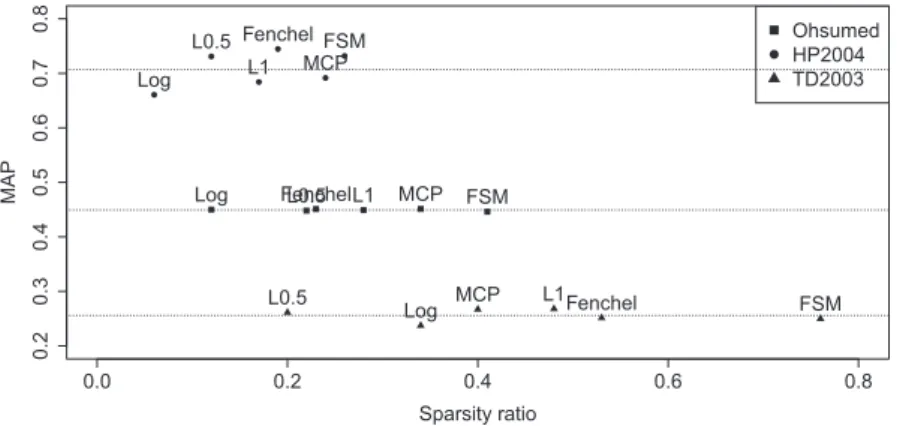
Fig. 3. MAP versus sparsity ratio for three representative datasets. Dotted lines represented average MAP obtained with the different algorithms.
state-of-the-art algorithms in most cases. They can lead to higher MAP or NDCG values, although the increase is not statistically significant.
C. Discussion
In the previous sections, we analyzed independently the ability of our framework to select only fewer features and their performance prediction. We showed that nonconvex penalties are competitive in reducing the number of features used by the learned models. We also pointed out that nonconvex penalties could lead to similar results as those of the best algorithms on most datasets.
Fig. 3 plots the MAP values against the sparsity ratio for three representative datasets. For each dataset, the average value of MAP among all the algorithms is represented by a dotted line. We restrict the number of datasets for readability reasons. Fig. 3 shows that the use of nonconvex regulariza-tions, especially the ℓpand log penalties, are highly compet-itive feature selection methods, both in terms of sparsity and prediction quality. Indeed, they achieve MAP and NDCG@10 performances that are similar to those of the state-of-the-art convex algorithms, while selecting half as many features on average on the datasets. On most datasets, the log and
ℓp penalties are the methods that select the smallest number of features, while the MAP remains stable. They can select up to six times fewer features than the other convex algo-rithms, without any significant degradation of the evaluation measures.
In the few cases where a significant decrease is observed, the degradation is usually small. On MQ2007 dataset, the MAP and NDCG@10 degradation observed when using the log penalty is less than 1%. It is similar to those obtained with convex algorithms, whereas the log penalty selects half as many features as the convex algorithms. On the same dataset, we observe a 3% decrease of the MAP and a 5.6% decrease of the NDCG@10 when using the ℓp penalty, but the algorithm selects up to 12 times fewer features than the convex approaches, and up to 4 times fewer features than the other nonconvex algorithms.
On HP2004, we observe a degradation of 11% of the MAP and of 4% of the NDCG when using the log penalty, but this method presents a better sparsity ratio and selects a
quarter as many features as the state-of-the-art methods. On the other hand, theℓp penalty provides as good results as the best method while selecting 37% fewer features than the best algorithm. On NP2003, we observe a degradation only for the
ℓp penalty, whereas the log penalty provides similar results as the convex methods and uses half as many features as the best algorithm FSMRank and the same number of features as FenchelRank. On this particular dataset, nonconvex methods do not perform as well as on the others, which may be due to the specificity of this dataset.
Moreover, we do not tune the specific parameter of non-convex regularizations but set them to default values that are usually used by the community. Results may be improved by an appropriate tuning of these parameters.
As a conclusion, the framework we proposed is able to provide similar results in terms of quality prediction com-pared to state-of-the-art approaches, while selecting half as many features. They are then competitive methods for feature selection in learning-to-rank.
VII. CONCLUSION
In this paper, we presented a general framework for fea-ture selection in learning-to-rank, by using SVM with sparse regularizations. We first proposed an accelerated proximal algorithm to solve the convex ℓ1 regularized problem. This algorithm has the same theoretical convergence rate as the state-of-the-art FenchelRank and FSMrank algorithms. We showed that a reweighted ℓ1 scheme can be used to solve nonconvex problems. This scheme was implemented into a second algorithm that solved problems with MCP, log and
ℓp, p < 1 penalties. To the best of our knowledge, it is the first work that proposes to consider nonconvex penal-ties for feature selection in learning to rank. We conducted experiments on two major benchmarks in learning to rank which include nine different datasets on which we evaluated the performance in terms of MAP and NDCG@10. We also evaluated the ability of our framework to induce sparsity into models.
We have shown that the nonconvex penalties lead to similar prediction quality irrespective of the evaluation measure used while using only half as many features as in convex methods. Our framework is then a novel, competitive, and effective
embedded method for feature selection in learning-to-rank. Its originality lies in the fact that it considers nonconvex regularizations to induce more sparsity into models without degradation of the prediction quality. Moreover, we provide publicly available software for the two proposed algorithms to promote reproducible research.
This paper and the contributions of Sun et al. [8] and
Lai et al. [9], [10] show the effectiveness of embedded
methods in the field of feature selection for learning-to-rank. More specifically, the use of sparse regularized SVMs seems to be a promising way to handle the issue of feature selection and dimensionality reduction in learning-to-rank. To the best of our knowledge, the work reported in this paper is the first that proposes a feature selection framework for learning-to-rank that is not restricted to the use of ℓ1-regularization. A wide range of issues still need to be explored. In future works, we plan to evaluate the impact of tuning the nonconvex regularizations parameters on both sparsity and prediction quality. An elaborate study of the computational times of the sparse leaning-to-rank algorithms could be conducted. Finally, as feature selection can be used to learn ranking function specific to a subset of queries, one of the most promising direction of work is the field of multitask learning. We plan to investigate the potential of a sparse regularized SVM algorithm using a fast iterative shrinkage threshold-ing framework, to be compared with an existthreshold-ing multitask algorithm [38]–[40].
REFERENCES
[1] T.-Y. Liu,Learning to Rank for Information Retrieval. New York, NY,
USA: Springer-Verlag, 2011.
[2] X. Geng, T.-Y. Liu, T. Qin, and H. Li, “Feature selection for ranking,” in
Proc. 30th Annu. Int. ACM SIGIR Conf. Res. Develop. Inf. Retr., 2007, pp. 407–414.
[3] G. Hua, M. Zhang, Y. Liu, S. Ma, and L. Ru, “Hierarchical feature selection for ranking,” inProc. 19th Int. Conf. World Wide Web, 2010, pp. 1113–1114.
[4] H. Yu, J. Oh, and W.-S. Han, “Efficient feature weighting methods for ranking,” in Proc. 18th ACM Conf. Inf. Knowl. Manag., 2009,
pp. 1157–1166.
[5] F. Pan, T. Converse, D. Ahn, F. Salvetti, and G. Donato, “Feature selection for ranking using boosted trees,” in Proc. 18th ACM Conf. Inf. Knowl. Manag., 2009, pp. 2025–2028.
[6] V. Dang and B. Croft, “Feature selection for document ranking using best first search and coordinate ascent,” inProc. SIGIR Workshop Feature Generat. Sel. Inf. Retr., 2010, pp. 1–5.
[7] T. Pahikkala, A. Airola, P. Naula, and T. Salakoski, “Greedy rankrls: A linear time algorithm for learning sparse ranking models,” inProc. SIGIR Workshop Feature Generat. Sel. Inf. Retr., 2010, pp. 11–18. [8] Z. Sun, T. Qin, Q. Tao, and J. Wang, “Robust sparse rank learning for
non-smooth ranking measures,” inProc. 32nd Int. ACM SIGIR Conf. Res. Develop. Inf. Retr., 2009, pp. 259–266.
[9] H. Lai, Y. Pan, C. Liu, L. Lin, and J. Wu, “Sparse learning-to-rank via an efficient primal-dual algorithm,”IEEE Trans. Comput., vol. 99, no. 6, pp. 1221–1233, Jun. 2012.
[10] H.-J. Lai, Y. Pan, Y. Tang, and R. Yu, “FSMRank: Feature selection algorithm for learning to rank,”IEEE Trans. Neural Netw. Learn. Syst.,
vol. 24, no. 6, pp. 940–952, Jun. 2013.
[11] R. Tibshirani, “Regression shrinkage and selection via the lasso,”J. R. Stat. Soc., Ser. B, vol. 58, no. 1, pp. 267–288, 1996.
[12] C.-H. Zhang, “Nearly unbiaised variable selection under minimax con-cave penalty,”Ann. Stat., vol. 38, no. 2, pp. 894–942, 2010.
[13] M. Kloft, U. Brefeld, S. Sonnenburg, and A. Zien, “lp-norm multiple kernel learning,”J. Mach. Learn. Res., vol. 12, pp. 953–997, Jul. 2011.
[14] D. Cossock and T. Zhang, “Subset ranking using regression,” inProc. 19th Annu. Conf. Learn. Theory, 2006, pp. 605–619.
[15] R. Nallapati, “Discriminative models for information retrieval,” inProc. 27th Annu. Int. ACM SIGIR Conf. Res. Develop. Inf. Retr., 2004, pp. 64–71.
[16] P. Li, C. J. C. Burges, and Q. Wu, “Mcrank: Learning to rank using multiple classification and gradient boosting,” in Proc. NIPS, 2007, pp. 897–904.
[17] K. Crammer and Y. Singer, “Pranking with ranking,” in Proc. Adv. Neural Inf. Process. Syst. 14. 2001, pp. 641–647.
[18] J. Fürnkranz and E. Hüllermeier,Preference Learning. New York, NY,
USA: Springer-Verlag, 2010.
[19] C. Burges, T. Shaked, E. Renshaw, A. Lazier, M. Deeds, N. Hamilton,
et al., “Learning to rank using gradient descent,” inProc. 22nd ICML, 2005, pp. 89–96.
[20] Y. Freund, R. Iyer, R. E. Schapire, and Y. Singer, “An efficient boosting algorithm for combining preferences,” J. Mach. Learn. Res., vol. 4, pp. 933–969, Dec. 2003.
[21] O. Chapelle and S. S. Keerthi, “Efficient algorithms for ranking with svms,”Inf. Retr., vol. 13, no. 3, pp. 201–215, Jun. 2010.
[22] T. Joachims, “Optimizing search engines using clickthrough data,” in
Proc. 18th ACM SIGKDD Int. Conf. Knowl. Discovery Data Mining,
2002, pp. 133–142.
[23] Z. Cao, T. Qin, T.-Y. Liu, M.-F. Tsai, and H. Li, “Learning to rank: From pairwise approach to listwise approach,” inProc. 24th Int. Conf. Mach. Learn., 2007, pp. 129–136.
[24] Y. Yue, T. Finley, F. Radlinski, and T. Joachims, “A support vector method for optimizing average precision,” inProc. 30th Annu. Int. ACM SIGIR Conf. Res. Develop. Inf. Retr., 2007, pp. 271–278.
[25] I. Guyon and A. Elisseeff, “An introduction to variable and feature selection,”J. Mach. Learn. Res.h, vol. 3, pp. 1157–1182, Mar. 2003. [26] J. H. Friedman, “Greedy function approximation: A gradient boosting
machine,”Ann. Stat., vol. 29, no. 5, pp. 1189–1232, 2000.
[27] M. R. Sikonja and K. Igor, “Theoretical and empirical analysis of relieff and RRefliefF,” Mach. Learn., vol. 53, nos. 1–2, pp. 23–69,
2003.
[28] R. Kohavi and G. H. John, “Wrappers for feature subset selection,”Artif. Intell., vol. 97, no. 1, pp. 273–324, 1997.
[29] H. Zou, “The adaptive lasso and its oracle properties,”J. Amer. Stat. Assoc., vol. 101, no. 476, pp. 1418–1429, 2006.
[30] G. Gasso, A. Rakotomamonjy, and S. Canu, “Recovering sparse sig-nals with a certain family of nonconvex penalties and DC program-ming,”IEEE Trans. Signal Process., vol. 57, no. 12, pp. 4686–4698, Dec. 2009.
[31] W. J. Fu, “Penalized regressions: The bridge versus the lasso,” J. Comput. Graph. Stat., vol. 7, no. 3, pp. 397–416, 1998.
[32] E. Candes, M. Wakin, and S. Boyd, “Enhancing sparsity by reweighted
ℓ1 minimization,”J. Fourier Anal. Applt., vol. 14, no. 5, pp. 877–905,
2008.
[33] J. Weston, A. Elisseeff, B. Schölkopf, and M. Tipping, “Use of the zero norm with linear models and kernel methods,”J. Mach. Learn. Res.,
vol. 3, pp. 1439–1461, Mar. 2003.
[34] F. Bach, R. Jenatton, J. Mairal, and G. Obozinski, “Convex optimization with sparsity-inducing norms,”Opt. Mach. Learn., vol. 3, pp. 19–53, Mar. 2011.
[35] A. Beck and M. Teboulle, “A fast iterative shrinkage-thresholding algorithm for linear inverse problems,”SIAM J. Imag. Sci., vol. 2, no. 1, pp. 183–202, Mar. 2009.
[36] P. D. Tao and L. T. H. An, “A DC optimization algorithm for solving the trust-region subproblem,”SIAM J. Opt., vol. 8, no. 2, pp. 476–505, 1998.
[37] D. Hunter and K. Lange, “A tutorial on MM algorithms,”Amer. Stat.,
vol. 58, no. 1, pp. 30–38, 2004.
[38] J. Bai, K. Zhou, G. Xue, H. Zha, G. Sun, B. Tseng,et al., “Multi-task
learning for learning to rank in web search,” inProc. 18th ACM Conf. Inf. Knowl. Manag., 2009, pp. 1549–1552.
[39] O. Chapelle, P. Shivaswamy, S. Vadrevu, K. Weinberger, Y. Zhang, and B. Tseng, “Multi-task learning for boosting with application to web search ranking,” inProc. 16th ACM SIGKDD Int. Conf. Mining, 2010, pp. 1189–1198.
[40] Y. Chang, J. Bai, K. Zhou, G.-R. Xue, H. Zha, and Z. Zheng, “Multi-task learning to rank for web search,”Pattern Recognit. Lett., vol. 33, no. 2, pp. 173–181, 2012.
Léa Laporte received the Dipl.-Ing. and M.S. degrees in applied mathematics from Institut National des Sciences Appliquées, Toulouse, France, in 2010. She is currently pursuing the Ph.D. degree with the Institut de Recherche en Informatique of Toulouse, UMR 5505 of the CNRS, Toulouse, under the supervision of S. Déjean and J. Mothe.
She also collaborates with Nomao, Toulouse, a French local search engine. Her current research interests include information retrieval, learning to rank, feature selection, and machine learning.
Rémi Flamary received the Dipl.-Ing. degree in electrical engineering, the M.S. degree in image processing from Institut National de Sciences Appliquées de Lyon, Lyon, France, in 2008, and the Ph.D. degree from the University of Rouen, Mont-Saint-Aignan, France, in 2011.
He has been an Assistant Professor with Univer-sité de Nice Sophia-Antipolis, Nice, France, and a member of the Lagrange Laboratory/Observatoire de la Côte d’Azur, Nice, since 2012. His current research interests include signal processing, machine learning, and image processing.
Stéphane Canu received the Ph.D. degree in sys-tem command from the Compiègne University of Technology, Compiègne, France, in 1986, and the French Habilitation degree from Paris 6 University, Paris, France.
He is a Professor of the LITIS Research Lab-oratory and the Information Technology Depart-ment, National Institute of Applied Science (INSA), Rouen, France. He joined the Faculty Department of computer science with the Compiegne University of Technology in 1987. In 1997, he joined the Rouen Applied Sciences National Institute, INSA, as a Full Professor, where he created the Information Engineering Department. He has been the Dean of this department until 2002 when he was named the Director of the Computing Service and Facilities Unit. In 2004, he joined the Machine Learning Group, ANU/NICTA, Canberra, Australia, with A. Smola and B. Williamson. He has published over 30 papers in refereed conference proceedings or journals in the areas of theory, algorithms and applications using kernel machines learning algorithm and other flexible regression methods. His current research interests include kernels machines, regularization, machine learning applied to signal processing, pattern classification, factorization for recommander systems, and learning for context aware applications.
Sébastien Déjean is a Statistician Research Engi-neer with the Institut of Mathematics of Toulouse, UMR5219 of the CNRS and University of Toulouse, Toulouse, France. Through his support activities to research, he contributes to various projects particu-larly in the fields of information retrieval systems and high throughput biology.
Josiane Motheis a Professor with École Supérieure du Professorat et de l’éducation, Université de Toulouse, Toulouse, France. She is leading the Infor-mation Retrieval and Mining Group, Institut de Recherche en Informatique de Toulouse, UMR 5505 of the CNRS, Toulouse. She is the co-director of the CNRS FREMIT research federation that groups together researchers from the Toulouse labs in math-ematics (IMT) and computer science (IRIT). Her current research interests include contextual infor-mation retrieval, query log and search results mining, and query difficulty prediction.