A feature selection method using improved regularized linear discriminant analysis

1 A Feature Selection Method Using Improved Regularized Linear Discriminant Analysis

Alok Sharma1,2,3_{, Kuldip K. Paliwal}2_{, Seiya Imoto}1_{, Satoru Miyano}1 1_{Laboratory of DNA Information Analysis, University of Tokyo, Japan}

2_{School of Engineering, Griffith University, Australia}

3_{School of Engineering and Physics, University of the South Pacific, Fiji} Abstract

Investigation of genes, using data analysis and computer based methods, has gained widespread attention in solving human cancer classification problem. DNA microarray gene expression datasets are readily utilized for this purpose. In this paper, we propose a feature selection method using improved regularized linear discriminant analysis technique to select important genes, crucial for human cancer classification problem. The experiment is conducted on several DNA microarray gene expression datasets and promising results are obtained when compared with several other existing feature selection methods.

Introduction

Feature selection methods play significant role in identifying crucial genes related to human cancers. It helps in understanding the gene regulation mechanism of cancer heterogeneity. DNA microarray gene expression data, consisting of several thousands of gene expression profiles, has been used widely in the past for cancer classification problem (Golub et al., 1999; Hastie et al., 2001; Khan et al., 2001; Armstrong, 2002). The high feature dimensionality (i.e., number of gene expression profiles) compared to the low number of samples, degrades the generalization performance of the classifier and increases its computational complexity. This problem is known as small sample size (SSS) problem (Fukunaga, 1990). These datasets along with feature selection methods provide vital information and assistance in comprehending biological and clinical characteristics. Since not all the genes are associated to cancer classification task, it is necessary to remove unimportant genes using feature selection or computational data analysis methods.

Various feature selection methods have been developed (Golub et al., 1999; Furey et al., 2000; Guyon et al., 2002; Li and Wong, 2003; Tan and Gilbert, 2003; Ding and Peng, 2003; Cong et al., 2005; Wang and Gehan, 2005; Banerjee et al., 2007; Pavlidis et al., 2001; Thomas et al., 2001; Pan, 2002; Dudoit et al., 2002; Saeys et al., 2007; Nie et al., 2010; Sharma et al., 2011, 2012a, 2012b, 2012c; Wu et al., 2011; Sharma et al., 2013a & 2013b), which can be broadly categorized into two main groups: filter methods and wrapper methods. The filter methods are classifier independent whereas the wrapper

2 methods are classifier dependent. Filter-based methods are computationally economical and follow an open-loop approach: the selection of genes is independent of the classifier. Therefore, the relevance of the extracted genes is obtained from a scoring procedure that uses intrinsic properties of the genes’ expression profiles. Wrapper-based methods (like SVM-RFE1_{) can provide high classification accuracy but are computationally} intensive and follow closed-loop approaches that depend on the classifier for gene selection. Although wrapper-based methods yield high classification accuracy, the gene sets they select do not necessarily possess biologically or clinically relevant attributes.

In this paper, we propose a feature selection method using regularized linear discriminant analysis (RLDA) technique (Friedman, 1989). This feature selection method falls under the filter method category as it does not require a classifier during training process to select features.

RLDA technique is one of the few pioneering techniques in the pattern classification literature. RLDA technique is used in the cases where SSS exist. In RLDA, a small perturbation, known as the regularization parameter 𝛼, is added to within-class scatter matrix 𝐒𝑊, to overcome SSS problem. The matrix 𝐒𝑊 is approximated by 𝐒𝑊+ 𝛼𝐈 and

the orientation matrix is computed by eigenvalue decomposition (EVD) of (𝐒𝑊+ 𝛼𝐈)−1𝐒𝐵,

where 𝐒𝐵 is between-class scatter matrix. RLDA has been applied in face recognition

and bioinformatics area (Dai and Yuen, 2003, 2007; Guo et al., 2007). In RLDA, it can be computationally expensive to find the optimum value of the parameter 𝛼 as heuristic approach (e.g. cross-validation procedure, Hastie et al., 2001) is applied. The value of the parameter could be sensitive and noisy especially when the number of training samples is scarce. In human cancer classification problem, the DNA microarray gene expression datasets, usually have very limited number of training samples which could adversely affect the classification performance of the RLDA technique.

In order to find the gene subset associated with human cancers, we first determine the value of 𝛼 for RLDA technique without using any heuristic approach. We call our procedure as improved RLDA technique. We use improved RLDA technique recursively to obtain crucial genes important for cancer classification task. The proposed feature

1 _{SVM-RFE (Guyon et al., 2002) is a wrapper based method. It is an iterative method which works}

backward from an initial set of features. The SVM aims to find maximum margin hyperplane between the two classes to minimize classification error using some kernel function.

3 selection method has been applied on several DNA microarray gene expression datasets and promising results have been obtained.

In the past, SVM has also applied recursively in SVM-RFE method (Guyon et al., 2002) to select features. SVM-RFE is a wrapper based method. It is an iterative method which works backward from an initial set of features. The SVM aims to find maximum margin hyperplane between the two classes to minimize classification error using some kernel function. The selection of features by SVM-RFE is computationally intensive. It has some other drawbacks as well due to applying maximum margin criterion between two classes (Zhou et al., 2010). On the other hand, RLDA based recursive feature selection method, separates the two classes by 1) shrinking within class variance, and 2) increasing the between class variance.

Basic descriptions

In this section we describe the basic notations used in the paper. Let X = {𝐱1, 𝐱2, … , 𝐱𝑛}

denote 𝑛 training samples (or feature vectors) in a 𝑑-dimensional space having class labels Ω = {𝜔1, 𝜔2, … , 𝜔𝑛}, where 𝜔 ∈ {1,2, … , 𝑐} and 𝑐 is the number of classes. The

dataset X can be subdivided into 𝑐 subsets X1, X2,…, Xc, where Xj belongs to class 𝑗 and consists of 𝑛𝑗 number of samples such that 𝑛 = ∑𝑐𝑗=1𝑛𝑗. The data subset Xj ⊂ X

and X1 ∪ X2 ∪…∪ Xc = X. If 𝛍_𝑗 = 1/𝑛_𝑗∑_{𝐱∈𝐗𝑗}𝐱 is the centroid of Xj and 𝛍 = 1/n ∑_𝐱∈𝐗𝐱 is the centroid of X, then the total scatter matrix 𝐒𝑇, within-class scatter matrix 𝐒𝑊

and between-class scatter matrix 𝐒𝐵 are defined as (Duda and Hart, 1973; Sharma and

Paliwal, 2008a, 2008b; Xu and Yan, 2009; Sharma and Paliwal, 2012; Huang, 2012a, 2012b) 𝐒𝑇 = ∑𝐱∈𝐗(𝐱 − 𝛍)(𝐱 − 𝛍)T, 𝐒𝑊= ∑ ∑ (𝐱 − 𝛍𝑗)(𝐱 − 𝛍𝑗) T 𝐱∈𝐗_𝑗 𝑐 𝑗=1 , and 𝐒𝐵= ∑𝑐𝑗=1𝑛𝑗(𝛍𝑗− 𝛍)(𝛍𝑗− 𝛍) T .

In SSS problem, 𝑑 > 𝑛, which will make scatter matrices singular. Let 𝑟𝑡 be the rank of

𝐒𝑇 matrix. The eigenvector decomposition of 𝐒𝑇 can be given as

𝐒𝑇 = [𝐔1, 𝐔2] [𝚲𝑇 ₀] [𝐔1 T

𝐔2T

], (1)

where 𝐔1∈ ℝ𝑑×𝑟𝑡 corresponds to eigenvalues 𝚲T and 𝐔2∈ ℝ𝑑×(𝑑−𝑟𝑡) corresponds to

the zero eigenvalues. The matrix 𝐔1 is the range space of 𝐒𝑇 and the matrix 𝐔2 is the

null space of 𝐒𝑇. Since the null space of 𝐒𝑇 does not contain any discriminant

4 𝑑-dimensional space to 𝑟𝑡-dimensional space by applying principal component analysis

(PCA) (Fukunaga, 1990; Sharma and Paliwal, 2007) as a pre-processing step. The range space of 𝐒𝑇 matrix, 𝐔1∈ ℝ𝑑×𝑟𝑡, will be used as a transformation matrix. In the reduced

dimensional space the scatter matrices can be computed by: 𝐒𝑊← 𝐔1T𝐒𝑊𝐔1 and

𝐒𝐵← 𝐔1T𝐒𝐵𝐔1. After this procedure 𝐒𝑊∈ ℝ𝑟𝑡×𝑟𝑡 and 𝐒𝐵∈ ℝ𝑟𝑡×𝑟𝑡 are reduced dimensional

within-class scatter matrix and reduced dimensional between-class scatter matrix, respectively.

Improved RLDA technique for feature selection

In RLDA, the regularization of within-class scatter matrix 𝐒𝑊 is carried out by adding

a perturbation term 𝛼 to the diagonal elements of 𝐒𝑊; i.e., 𝐒̂𝑊= 𝐒𝑊+ 𝛼𝐈. The addition

of 𝛼 will make within-class scatter non-singular and invertible. This would help to maximize the modified Fisher’s criterion

𝐽(𝐰, 𝛼) = 𝐰

T_𝐒 𝐵𝐰

𝐰T_(𝐒

𝑊+ 𝛼𝐈)𝐰 , (2)

where 𝐰 ∈ ℝ𝑟_𝑡×1 _{is the orientation vector. In order to avoid any heuristic approach in}

the determination of the parameter 𝛼, we solve equation 2 in the following manner. Let us denote function 𝑓 = 𝐰T_𝐒

𝐵𝐰 and a constraint function 𝑔 = 𝐰T(𝐒𝑊+ 𝛼𝐈)𝐰 − 𝑐 = 0,

where 𝑐 > 0 be any constant. To find the constrained relative-maximum of function 𝑓 under constrained curve 𝑔, we can use the method of Lagrange multipliers (Anton, 1995) as follows:

𝜕𝑓 𝜕𝐰= 𝜆

𝜕𝑔

𝜕𝐰 , (3)

where 𝜆 ≠ 0 is the Lagrange’s multiplier. Equation 3 is the Lagrange’s function where we are interested in finding the parameters (𝐰, 𝜆) that maximizes function 𝑓 under the constrained curve 𝑔. Substituting 𝑓 = 𝐰T_𝐒

𝐵𝐰 and 𝑔 = 𝐰T(𝐒𝑊+ 𝛼𝐈)𝐰 − 𝑐 in equation

3, we get

2𝐒𝐵𝐰 = 𝜆(2𝐒𝑊𝐰 + 2𝛼𝐰),

or (1_𝜆𝐒𝐵− 𝐒𝑊)𝐰 = 𝛼𝐰. (4)

The value of 𝛼𝐰 can be substituted in the constraint function 𝑔, this will give us, 𝐰T_𝐒

𝐵𝐰 = λ𝑐. (5)

Also from the constraint function 𝐰T_(𝐒

𝑊+ 𝛼𝐈)𝐰 − 𝑐 = 0, we get 𝐰T𝐒̂𝑊𝐰 = 𝑐. Dividing

this term in equation 5, we get λ = 𝐰T𝐒B𝐰

𝐰T_𝐒̂ 𝑊𝐰

. (6)

5 Lagrange’s multiplier (in equation 4), and 2) the right-hand side is same as the Fisher’s modified criterion defined in equation 2. In order to obtain the value of 𝜆 in equation 6, we need to estimate 𝐒̂𝑊. If the matrix is not regularize (i.e., 𝛼 = 0) then 𝐒̂𝑊= 𝐒𝑊. By

this substitution, we can obtain approximate value of 𝜆 by maximizing 𝐰T_𝐒

B𝐰/𝐰T𝐒𝑊𝐰.

Now to find the maximum value of 𝐰T_𝐒

B𝐰/𝐰T𝐒𝑊𝐰, we must have eigenvector 𝐰

corresponding to the leading eigenvalue of 𝐒W−1𝐒B. However, since 𝐒𝑊 is singular and

non-invertible, 𝐒𝑊+ can be used in place of 𝐒𝑊−1, where 𝐒𝑊+ is the pseudoinverse of 𝐒𝑊.

From the EVD of 𝐒𝑊+𝐒𝐵, we can find 𝜆𝑚𝑎𝑥 which is the largest eigenvalue of 𝐒𝑊+𝐒𝐵. The

value of 𝜆𝑚𝑎𝑥 can be substituted in equation 4 (where 𝜆 = 𝜆𝑚𝑎𝑥), this will enable us to

find the value of 𝛼 by doing EVD of (1_𝜆𝐒𝐵− 𝐒𝑊). If 𝑟𝑏= 𝑟𝑎𝑛𝑘(𝐒𝐵) then EVD of

(1_𝜆𝐒𝐵− 𝐒𝑊) will give 𝑟𝑏 finite eigenvalues. Since the leading eigenvalue will correspond

to the most discriminant eigenvector (Fukunaga, 1990; Sharma and Paliwal, 2007), 𝛼 is taken to be the leading eigenvalue. Once the value of 𝛼 is determined, the orientation vector 𝐰 can be solved from

(𝐒𝑊+ 𝛼𝐈)−𝟏𝐒𝐵𝐰 = γ𝐰. (7)

It can be shown from Lemma 1 that for improved RLDA technique, its maximum eigenvalue is approximately equal to the highest (finite) eigenvalue of Fisher’s criterion.

Lemma 1: The highest eigenvalue of improved RLDA is approximately equivalent to the highest (finite) eigenvalue of Fisher’s criterion.

Proof 1: From equation 7,

𝐒𝐵𝐰𝑗= 𝛾𝑗(𝐒𝑊+ 𝛼𝐈)𝐰𝑗, (8)

where 𝛼 is the maximum eigenvalue of (1/𝜆𝑚𝑎𝑥𝐒𝐵− 𝐒𝑊) (from equation 4); 𝜆𝑚𝑎𝑥 ≥ 0

is approximately the highest eigenvalue of Fisher’s criterion 𝐰T_𝐒

𝐵𝐰/𝐰T𝐒𝑊𝐰 (since

𝜆𝑚𝑎𝑥 is the largest eigenvalue of 𝐒𝑊+𝐒𝐵) (Liu et al., 2007); 𝑗 = 1 … 𝑟𝑏 and 𝑟𝑏= 𝑟𝑎𝑛𝑘(𝐒𝐵).

Substituting 𝛼𝐰 = (1/𝜆𝑚𝑎𝑥𝐒𝐵− 𝐒𝑊)𝐰 (from equation 4, where 𝜆 = 𝜆𝑚𝑎𝑥) into equation

8, we get,

𝐒𝐵𝐰𝑚= 𝛾𝑚𝐒𝑊𝐰𝑚+ 𝛾𝑚(1/𝜆𝑚𝑎𝑥𝐒𝐵− 𝐒𝑊)𝐰𝑚,

or (𝜆𝑚𝑎𝑥− 𝛾𝑚)𝐒𝐵𝐰𝑚= 0.

where 𝛾𝑚= max (𝛾𝑗) and 𝐰𝑚 is the corresponding eigenvector. Since 𝐒𝐵𝐰𝑚≠ 0 (from

equation 5), 𝛾𝑚= 𝜆𝑚𝑎𝑥 and 𝛾𝑗< 𝜆𝑚𝑎𝑥, where 𝑗 ≠ 𝑚. This concludes the proof.

Corollary 1: The value of regularization parameter is non-negative; i.e., 𝛼 ≥ 0 for 𝑟𝑤≤ 𝑟𝑡, where 𝑟𝑡= 𝑟𝑎𝑛𝑘(𝐒𝑇) and 𝑟𝑤= 𝑟𝑎𝑛𝑘(𝐒𝑊).

6 Computing equation 7 for all the values of 𝛾 will give the orientation matrix 𝐖 ∈ ℝ𝑟_𝑡×𝑟_{𝑏, having 𝐰 as its column vectors. The orientation matrix 𝐖 is in 𝑟}

𝑡-dimensional

space, however, it can be transformed to 𝑑-dimensional space by 𝐖 ← 𝐔1𝐖. Therefore,

we get 𝐖 ∈ ℝ𝑑×𝑟_{𝑏. Let a column vector 𝐰 ∈ 𝐖 be used to transform 𝑑-dimensional}

space to 1-dimensional space and 𝐱 ∈ 𝐗 be any feature vector, we have 𝑦 = 𝐰T_𝐱,

or 𝑦 = ∑𝑑𝑖=1𝑤𝑖𝑥𝑖, (9)

where 𝑤𝑖 and 𝑥𝑖 are the elements of 𝐰 and 𝐱, respectively. It can be envisaged that if

|𝑤𝑖𝑥𝑖| ≈ 0 (where | ∙ | is the absolute value), then the 𝑖th element is not contributing

for the value of 𝑦 in equation 9; i.e., it can be discarded without sacrificing much information. This concept can be extended for the orientation matrix 𝐖 and dataset 𝐗 as

𝑧𝑖= ∑𝑟𝑘=1𝑏 ∑𝑛𝑗=1|𝑤𝑖𝑘𝑥𝑖𝑗| (10)

where 𝑖 = 1,2, … , 𝑑. If 𝑧𝑖 ≈ 0, then 𝑖th feature can be discarded. Equation 10 can be

applied recursively to discard unimportant features as follows:

Step 0. Define 𝑞 ∈ (𝑛, 𝑑)2 _{and set 𝑙 = 𝑑.}

Step 1. Compute 𝐖 ∈ ℝ𝑙×𝑟_{𝑏 (see Table 1).}

Step 2. Compute 𝑧𝑖 using equation 10 for 𝑖 = 1,2, … , 𝑙.

Step 3. Sort 𝑧𝑖 in descending order; i.e., if 𝑠 = 𝑠𝑜𝑟𝑡(𝑧𝑖) then 𝑠1> 𝑠2> ⋯ > 𝑠𝑙.

Step 4. Discard least important feature corresponding to 𝑠𝑙. Let the cardinality of the

remaining feature set be 𝑙 − 1 and data subset be 𝐗𝑙−1∈ ℝ𝑙×𝑛.

Step 5. Conduct 𝐗 ← 𝐗𝑙−1 and 𝑙 ← 𝑙 − 1.

Step 6. Continue Steps 1-5 until 𝑙 = 𝑞.

The above process will give 𝑞-features with the data subset 𝐗𝑞∈ ℝ𝑞×𝑛, which can be

used by a classifier to obtain classification performance.

Table 1: Computation of the orientation matrix 𝐖 using improved RLDA technique.

2

Since RLDA or Improved RLDA is a method for solving small sample size (SSS) problem, the value of q has to be in (𝑛, 𝑑).

7

Step 1. Compute range space of total scatter matrix 𝐒𝑇, 𝐔1∈ ℝ𝑑×𝑟𝑡, by applying PCA,

where 𝑟𝑡= 𝑟𝑎𝑛𝑘(𝐒𝑇). Using 𝐔1, compute between-class scatter matrix and

within-class scatter matrix in 𝑟𝑡 dimensional space: 𝐒𝐵← 𝐔1T𝐒𝐵𝐔1 and

𝐒𝑊← 𝐔1T𝐒𝑊𝐔1, where 𝐒𝐵∈ ℝ𝑟𝑡×𝑟𝑡 and 𝐒𝑊∈ ℝ𝑟𝑡×𝑟𝑡.

Step 2. Perform EVD of 𝐒𝑊+𝐒𝐵 to find the highest eigenvalue 𝜆𝑚𝑎𝑥.

Step 3. Perform EVD of (1/𝜆𝑚𝑎𝑥𝐒𝐵− 𝐒𝑊) to find its highest eigenvalue, denote it as 𝛼. Step 4. Perform EVD of (𝐒𝑊+ 𝛼𝐈)−𝟏𝐒𝐵 to find 𝑟𝑏 eigenvectors 𝐰𝑗 ∈ ℝ𝑟𝑡×1

corresponding to the leading eigenvalues, where 𝑟𝑏= 𝑟𝑎𝑛𝑘(𝐒𝐵) . The

eigenvectors 𝐰𝑗 are column vectors of the orientation matrix 𝐖′∈ ℝ𝑟𝑡×𝑟𝑏. Step 5. Compute the orientation matrix 𝐖 ∈ ℝ𝑑×𝑟_{𝑏 in 𝑑-dimensional space: 𝐖 =}

𝐔1𝐖′.

The computational requirement for Step 1 of the technique (Table 1) would be 𝑂(𝑑𝑛2_);

for Step 2 would be 𝑂(𝑛3_{); for Step 3 would be 𝑂(𝑛}3_{); for Step 4 would be 𝑂(𝑛}3_{); and,}

for Step 5 would be 𝑂(𝑑𝑛2_{). Therefore, the total estimated for SSS case (𝑑 ≫ 𝑛) would}

be 𝑂(𝑑𝑛2_{). If the 𝑞 features are to be selected from the total 𝑑 features then total}

estimated computational complexity would be 𝑂(𝑑𝑛2_{(𝑑 − 𝑙)).}

Experimentation

In this experiment we have utilized three DNA microarray gene expression datasets3_. The description of these datasets is given as follows:

SRBCT dataset (Khan et al., 2001): the small round blue-cell tumor dataset consists of 83 samples with each having 2308 genes. This is a four class classification problem. The tumors are Burkitt lymphoma (BL), the Ewing family of tumors (EWS), neuroblastoma

(NB) and rhabdomyosarcoma (RMS). There are 63 samples for training and 20 samples for testing. The training set consists of 8, 23, 12 and 20 samples of BL, EWS, NB and RMS respectively. The test set consists of 3, 6, 6 and 5 samples of BL, EWS, NB and RMS respectively.

MLL Leukemia dataset (Armstrong et al., 2002): this dataset has 3 classes namely ALL,

3

Most of the datasets are downloaded from the Kent Ridge Bio-medical Dataset (KRBD) (http://datam.i2r.a-star.edu.sg/datasets/krbd/). The datasets are transformed or reformatted and made available by KRBD repository and we have used them without any further preprocessing. Some datasets which are not available on KRBD repository are downloaded and directly used from respective authors’ supplement link. The URL addresses for all the datasets are given in the Reference Section.

8 MLL and AML. The training set contains 57 leukemia samples (20 ALL, 17 MLL and 20 AML) whereas the test set contains 15 samples (4 ALL, 3 MLL and 8 AML). The dimension of the MLL dataset is 12582.

Acute Leukemia dataset (Golub et al., 1999): this dataset consists of DNA microarray gene expression data of human acute leukemia for cancer classification. Two types of acute leukemia data are provided for classification namely acute lymphoblastic leukemia (ALL) and acute myeloid leukemia (AML). The dataset is subdivided into 38 training samples and 34 test samples. The training set consists of 38 bone marrow samples (27 ALL and 11 AML) over 7129 probes. The test set consists of 34 samples with 20 ALL and 14 AML, prepared under different experimental conditions. All the samples have 7129 dimensions and all are numeric.

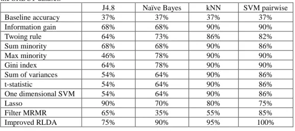
The classification performance of the proposed feature selection method has been gauged by using the above three datasets. Tables 2, 3 and 4 show classification accuracy of the proposed method compared with several other existing feature selection methods on the SRBCT, MLL and Acute Leukemia datasets, respectively4_{. Four classifiers from} WEKA (http://www.cs.waikato.ac.nz/ml/weka/) used are J4.8, Naïve Bayes, kNN (where 𝑘 = 1) and SVM pairwise. The classification accuracy for the SRBCT and MLL datasets is obtained from Tao et al. 2004. For all the datasets, the features are ranked by Rankgene program (Su et al., 2003). The Rankgene program computes the features for the following feature selection methods: Information gain, Twoing rule, Sum minority, Max minority, Gini index, Sum of variances, t-statistic and One-dimensional SVM (Su et al., 2003). For all the datasets 150 genes are selected as selected by Tao et al., 2004. In addition, Lasso (Tibshirani, 1996) and filter MRMR (Peng et al., 2005) are used for feature selection. The Lasso method deflates the collinearity effect on the features. It produces sparse parameters that can be used to identify important genes. The number of features selected by Lasso on SRBCT, MLL and Acute Leukamia is 38, 39 and 165_, respectively. The filter MRMR method select features based on maximal statistical dependency criterion based on mutual information. It can be observed from Table 2 that

4 _{The cross-validation based results are shown in Appendix-I Section. The comparison of improved}

RLDA with different values of regularization parameter has been shown in Appendix-II Section.

5 _{Note that for all the feature selection methods except Lasso method the number of selected features is}

150 (in Tables 2,3 and 4). The Lasso method itself obtains the optimal number of selected features and therefore cannot be adjusted for a predefined number of selected features.

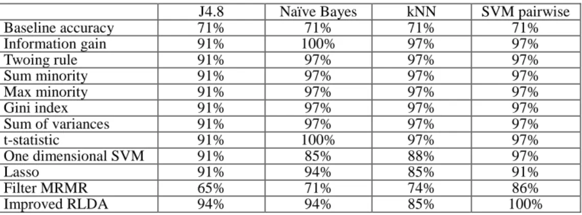
9 the proposed method achieves 75% classification accuracy using the J4.8 classifier; 90% classification accuracy using the Naïve Bayes classifier; 95% classification accuracy using the kNN classifier and 100% classification accuracy by the SVM pairwise classifier. In the three out of four cases the classification accuracy obtained by improved RLDA is the highest. Similarly, the classification accuracy on the MLL dataset (Table 3) is the highest for improved RLDA in three out of four cases method when compared with several other feature selection methods using four distinct classifiers. On the Acute Leukemia dataset (Table 4), the classification accuracy of improved RLDA is the highest for the J4.8 classifier (94%) and the SVM pairwise classifier (100%). In total of 12 cases (Tables 2-4), improved RLDA is giving highest results in eight cases. It can, therefore, be concluded that the proposed method is exhibiting promising results.

Table 2: The classification accuracy of various feature selection methods using four distinct classifiers on the SRBCT dataset.

J4.8 Naïve Bayes kNN SVM pairwise

Baseline accuracy 37% 37% 37% 37% Information gain 68% 68% 90% 90% Twoing rule 64% 73% 86% 82% Sum minority 68% 68% 90% 86% Max minority 46% 78% 90% 90% Gini index 64% 78% 90% 90% Sum of variances 54% 64% 90% 86% t-statistic 54% 64% 90% 86% One dimensional SVM 54% 64% 90% 86% Lasso 90% 70% 80% 75% Filter MRMR 65% 35% 55% 85% Improved RLDA 75% 90% 95% 100%

Table 3: The classification accuracy of various feature selection methods using four distinct classifiers on the MLL dataset.

J4.8 Naïve Bayes kNN SVM pairwise

Baseline accuracy 35% 35% 35% 35% Information gain 60% 74% 86% 100% Twoing rule 60% 86% 86% 100% Sum minority 68% 26% 80% 80% Max minority 74% 34% 74% 80% Gini index 60% 68% 86% 100% Sum of variances 60% 54% 86% 100% t-statistic 60% 54% 86% 100% One dimensional SVM 60% 54% 86% 100% Lasso 87% 100% 93% 93% Filter MRMR 100% 100% 93% 100% Improved RLDA 100% 93% 100% 100%

Table 4: The classification accuracy of various feature selection methods using four distinct classifiers on the Acute Leukemia dataset.

10

J4.8 Naïve Bayes kNN SVM pairwise

Baseline accuracy 71% 71% 71% 71% Information gain 91% 100% 97% 97% Twoing rule 91% 97% 97% 97% Sum minority 91% 97% 97% 97% Max minority 91% 97% 97% 97% Gini index 91% 97% 97% 97% Sum of variances 91% 97% 97% 97% t-statistic 91% 100% 97% 97% One dimensional SVM 91% 85% 88% 97% Lasso 91% 94% 85% 91% Filter MRMR 65% 71% 74% 86% Improved RLDA 94% 94% 85% 100%

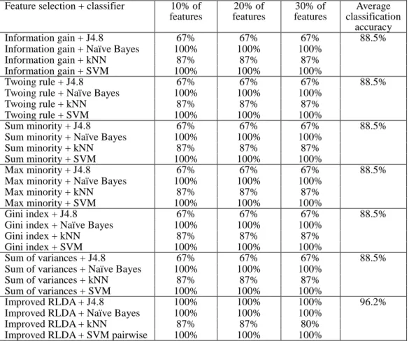
Next, we considered different number of selected features by Improved RLDA and several feature selection method, and shown the evolution of the performance of the classifiers with respect to the number of selected features. The results are shown in Tables 5, 6 and 7. It can be observed from the Tables 5-7 that in most of the cases the average classification accuracy for Improved RLDA is consistently higher than other feature selection methods.

Table 5: The classification accuracy as a function of the number of selected features of Improved RLDA and several feature selection methods using four distinct classifiers on the SRBCT dataset.

Feature selection + classifier 10% of features 20% of features 30% of features Average classification accuracy Information gain + J4.8 65% 65% 65% 81.7%

Information gain + Naïve Bayes 85% 65% 55%

Information gain + kNN 100% 90% 90%

Information gain + SVM 100% 100% 100%

Twoing rule + J4.8 65% 65% 65% 82.1%

Twoing rule + Naïve Bayes 85% 70% 55%

Twoing rule + kNN 100% 90% 90%

Twoing rule + SVM 100% 100% 100%

Sum minority + J4.8 60% 65% 65% 79.6%

Sum minority + Naïve Bayes 75% 55% 55%

Sum minority + kNN 100% 95% 85%

Sum minority + SVM 100% 100% 100%

Max minority + J4.8 65% 65% 65% 83.3%

Max minority + Naïve Bayes 95% 65% 65%

Max minority + kNN 100% 90% 90%

Max minority + SVM 100% 100% 100%

Gini index + J4.8 65% 75% 75% 85.8%

Gini index + Naïve Bayes 90% 70% 65%

Gini index + kNN 100% 95% 95%

Gini index + SVM 100% 100% 100%

Sum of variances + J4.8 65% 65% 65% 79.2%

Sum of variances + Naïve Bayes 60% 60% 55%

Sum of variances + kNN 100% 90% 90%

Sum of variances + SVM 100% 100% 100%

Improved RLDA + J4.8 75% 75% 75% 88.3%

Improved RLDA + Naïve Bayes 90% 90% 70%

Improved RLDA + kNN 95% 95% 95%

11 Table 6: The classification accuracy as a function of the number of selected features of Improved RLDA and several feature selection methods using four distinct classifiers on the MLL dataset.

Feature selection + classifier 10% of features 20% of features 30% of features Average classification accuracy Information gain + J4.8 67% 67% 67% 88.5%

Information gain + Naïve Bayes 100% 100% 100%

Information gain + kNN 87% 87% 87%

Information gain + SVM 100% 100% 100%

Twoing rule + J4.8 67% 67% 67% 88.5%

Twoing rule + Naïve Bayes 100% 100% 100%

Twoing rule + kNN 87% 87% 87%

Twoing rule + SVM 100% 100% 100%

Sum minority + J4.8 67% 67% 67% 88.5%

Sum minority + Naïve Bayes 100% 100% 100%

Sum minority + kNN 87% 87% 87%

Sum minority + SVM 100% 100% 100%

Max minority + J4.8 67% 67% 67% 88.5%

Max minority + Naïve Bayes 100% 100% 100%

Max minority + kNN 87% 87% 87%

Max minority + SVM 100% 100% 100%

Gini index + J4.8 67% 67% 67% 88.5%

Gini index + Naïve Bayes 100% 100% 100%

Gini index + kNN 87% 87% 87%

Gini index + SVM 100% 100% 100%

Sum of variances + J4.8 67% 67% 67% 88.5%

Sum of variances + Naïve Bayes 100% 100% 100%

Sum of variances + kNN 87% 87% 87%

Sum of variances + SVM 100% 100% 100%

Improved RLDA + J4.8 100% 100% 100% 96.2%

Improved RLDA + Naïve Bayes 100% 100% 100%

Improved RLDA + kNN 87% 87% 80%

Improved RLDA + SVM pairwise 100% 100% 100%

Table 7: The classification accuracy as a function of the number of selected features of Improved RLDA and several feature selection methods using four distinct classifiers on the Acute Leukemia dataset.

Feature selection + classifier 10% of features 20% of features 30% of features Average classification accuracy Information gain + J4.8 91% 91% 91% 90.6%

Information gain + Naïve Bayes 97% 100% 100%

Information gain + kNN 77% 79% 79%

Information gain + SVM 97% 94% 91%

Twoing rule + J4.8 91% 91% 91% 89.1%

Twoing rule + Naïve Bayes 94% 97% 97%

Twoing rule + kNN 77% 76% 79%

Twoing rule + SVM 97% 91% 88%

Sum minority + J4.8 91% 91% 91% 88.3%

Sum minority + Naïve Bayes 94% 97% 97%

Sum minority + kNN 77% 73% 73%

Sum minority + SVM 97% 91% 88%

Max minority + J4.8 91% 91% 91% 89.2%

Max minority + Naïve Bayes 94% 97% 97%

Max minority + kNN 77% 77% 79%

Max minority + SVM 97% 91% 88%

Gini index + J4.8 91% 91% 91% 88.0%

Gini index + Naïve Bayes 94% 97% 97%

Gini index + kNN 79% 70% 70%

12

Sum of variances + J4.8 91% 91% 91% 89.2%

Sum of variances + Naïve Bayes 94% 97% 97%

Sum of variances + kNN 77% 77% 79%

Sum of variances + SVM 97% 91% 88%

Improved RLDA + J4.8 91% 91% 91% 92.5%

Improved RLDA + Naïve Bayes 97% 100% 100%

Improved RLDA + kNN 88% 79% 82%

Improved RLDA + SVM pairwise 97% 97% 97%

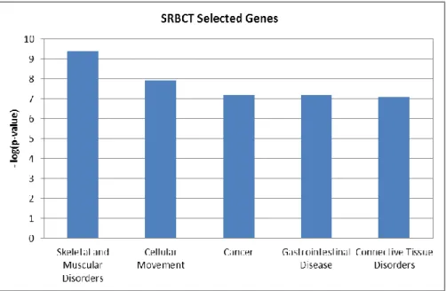
Furthermore, we conducted experiments to see the biological significance of the selected features by the proposed method. We use SRBCT data as a prototype to show the biological significance using Ingenuity Pathway Analysis6_{. The selected 150 features} from the proposed algorithm are used for this purpose. Out of 150 genes, 10 genes were found unmapped in IPA. The top five high level biological functions obtained are shown in Figure 1. In the figure, the y-axis denotes the negative of logarithm of p-values and x-axis denotes the high level functions. Since the cancer function is of paramount interest, we investigated them further. There are 61 cancer sub-functions obtained from the experiment. Top 25 cancer sub-functions with significant p-values are shown in Table 8. In IPA, the p-value reflects the enrichment of a given function to a set of focused genes. The smaller the p-value is, the less likely that the association is random, and the more significant the association. In general p-values less than 0.05 indicate a statistically significant, non-random association. The p-value is calculated using the right-tailed Fisher exact test (IPA, Available at: http://www.ingenuity.com) (Sharma et al., 2012a; 2012b). In the table, the p-values and the number of selected genes are depicted corresponding to the selected functions. The selected genes by the proposed method provide significant p-values above the threshold (as specified in IPA). This shows that the features selected by the proposed method contain useful information for discriminatory purpose and have biological significance.

6 _{Ingenuity Pathway Analysis (IPA) (http://www.ingenuity.com) is a software that helps researchers to}

model, analyze, and understand the complex biological and chemical systems at the core of life science research. IPA has been broadly adopted by the life science research community. IPA helps to understand complex 'omics data at multiple levels by integrating data from a variety of experimental platforms and providing insight into the molecular and chemical interactions, cellular phenotypes, and disease processes of the system. IPA provides insight into the causes of observed gene expression changes and into the predicted downstream biological effects of those changes. Even if the experimental data is not available, IPA can be used to intelligently search the Ingenuity Knowledge Base for information on genes, proteins, chemicals, drugs, and molecular relationships to build biological models or to get up to speed in a relevant area of research. IPA provides the right biological context to facilitate informed decision-making, advance research project design, and generate new testable hypotheses.

13 Figure 1: Top five high level biological function on selected 150 genes of SRBCT by Improved RLDA based feature selection method.

Table 8: Cancer sub-functions

Functions p-value # Selected Genes

metastatic colorectal cancer 6.99E-08 12

tumorigenesis 1.01E-07 62

neoplasia 5.05E-07 59

cancer 6.97E-07 58

uterine cancer 2.87E-06 19

benign tumor 3.75E-06 17

leiomyomatosis 1.06E-05 12

carcinoma 1.11E-05 47

adenocarcinoma 1.81E-05 17

gastrointestinal tract cancer 2.60E-05 24

colorectal cancer 3.46E-05 22

uterine leiomyoma 5.62E-05 10

metastasis 6.11E-05 13

genital tumor 6.69E-05 22

prostate cancer 1.42E-04 16

trisomy 8 myelodysplastic syndrome 2.25E-04 2 central nervous system tumor 2.87E-04 10

digestive organ tumor 3.21E-04 27

breast cancer 3.41E-04 20

brain cancer 4.28E-04 9

leukemia 6.88E-04 11

hematologic cancer 7.14E-04 14

endometrial carcinoma 8.86E-04 8

neuroblastoma 1.25E-03 5

14

endocrine gland tumor 1.42E-03 11

tumorigenesis of carcinoma 1.54E-03 2

B-cell leukemia 1.68E-03 6

entrance of tumor cell lines 2.04E-03 2

endometrial cancer 2.12E-03 7

We have also carried out sensitivity analysis to check the robustness of the proposed method. For this purpose, we use the SRBCT dataset as a prototype and select top 100 genes. After this selection, we contaminate the dataset by adding Gaussian noise, then applied the method again to find the top 100 genes. The generated noise levels are 1%, 2% and 5% of the standard deviation of the original gene expression values. The number of genes which are common after contamination and before contamination is noted. This contamination of data and selection of genes are repeated 20 times. The average number of genes over 20 iterations is depicted in Figure 2. It can be observed from the figure that the proposed method is able to capture the majority of the original genes in the noisy environmental condition.

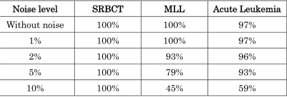
In order to check the sensitivity analysis with respect to the classification accuracy, we contaminated the dataset by adding Gaussian noise (as above) and selected 150 features using the improved RLDA technique. The classification accuracy is obtained by using the SVM-pairwise classifier. The results are shown in Table 9. It can observed from Table 9 that for low level noise the degradation in classification performance is not enough. But when the noise level increases the classification accuracy deteriorates (especially on the MLL dataset and the Acute Leukemia dataset).

Table 9: Sensitivity analysis with respect to classification accuracy on the SRBCT, MLL and Acute Leukemia dataset

Noise level SRBCT MLL Acute Leukemia

Without noise 100% 100% 97%

1% 100% 100% 97%

2% 100% 93% 96%

5% 100% 79% 93%

15 Figure 2:Sensitivity analysis for the proposed feature selection method on the SRBCT dataset at different noise levels. The y-axis depicts the average number of common genes over 20 iterations and x-axis depicts the added noise in percentage.

Next, we carried out experimentation to obtain ROC curve and AUC analysis. For the ROC curve, we use sensitivity and specificity as the two measures. The sensitivity is given as 𝑇𝑟𝑢𝑒 𝑃𝑜𝑠𝑖𝑡𝑖𝑣𝑒/(𝑇𝑟𝑢𝑒 𝑃𝑜𝑠𝑖𝑡𝑖𝑣𝑒 + 𝐹𝑎𝑙𝑠𝑒 𝑁𝑒𝑔𝑎𝑡𝑖𝑣𝑒) and the specificity is given as 𝑇𝑟𝑢𝑒 𝑛𝑒𝑔𝑎𝑡𝑖𝑣𝑒/(𝑇𝑟𝑢𝑒 𝑁𝑒𝑔𝑎𝑡𝑖𝑣𝑒 + 𝐹𝑎𝑙𝑠𝑒 𝑃𝑜𝑠𝑖𝑡𝑖𝑣𝑒). We varied the noise level and select 150 genes using improved RLDA and then use SVM-pairwise to compute sensitivity and specificity. The ROC curve is shown in Figure 3. This curve shows the trade-off between sensitivity and specificity. The AUC provides the overall accuracy and is a useful parameter for comparing the performance. The high value of AUC parameter indicates high accuracy. The value of AUC is computed to be 0.9674 which is promising.

84 86 88 90 92 94 96 98 100 1 2 3 4 5 A ve rag e n u m be r of c om mo n g en es

16 Figure 3: The ROC curve

Conclusion

In this paper, we presented a feature selection method using improved regularized linear discriminant analysis technique. Three DNA microarray gene expression datasets have been utilized to see the performance of the proposed method. It was observed that the method is achieving encouraging classification accuracy using small number of selected gene. The biological significance has also been demonstrated by performing functional analysis. Moreover, robustness of the method was exhibited by conducting sensitivity analysis and encouraging results are obtained. The sensitivity analysis with respect to classification accuracy and ROC curve have also been discussed.

Appendix I

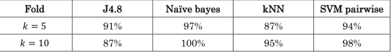
In this section, we use cross-validation procedure to compute average classification accuracy using four distinct classifiers and the proposed feature selection method. Three datasets have been used for this purpose are SRBCT, MLL and Acute Leukemia. The classification accuracy using fold 𝑘 = 5 and fold 𝑘 = 10 are given in Tables A1, A2 and A3. It can be observed that the classification accuracy obtained by 𝑘-fold cross-validation procedure is comparably similar to the classification accuracy obtained in Tables 2-4. 0 0.005 0.01 0.015 0.02 0.025 0.03 0.035 0.04 0.045 0.05 0 0.1 0.2 0.3 0.4 0.5 0.6 0.7 0.8 0.9 1 1-Specificity S e n s it iv it y AUC = 0.9674

17 Table A1: 𝑘-fold cross-validation using improved RLDA and four distinct classifiers on the SRBCT dataset.

Fold J4.8 Naïve bayes kNN SVM pairwise

𝑘 = 5 80% 89% 92% 100%

𝑘 = 10 88% 92% 95% 100%

Table A2: 𝑘-fold cross-validation using improved RLDA and four distinct classifiers on the MLL dataset.

Fold J4.8 Naïve bayes kNN SVM pairwise

𝑘 = 5 91% 94% 94% 95%

𝑘 = 10 87% 93% 95% 97%

Table A3: 𝑘-fold cross-validation using improved RLDA and four distinct classifiers on the Acute Leukemia dataset.

Fold J4.8 Naïve bayes kNN SVM pairwise

𝑘 = 5 91% 97% 87% 94%

𝑘 = 10 87% 100% 95% 98%

Appendix II

In this appendix, we compare different values of regularization parameter with the proposed improved RLDA technique. In order to show this, we computed classification accuracy on four different values of 𝛼 for RLDA technique. These are 𝛿 = [0.001,0.01,0.1,1], where 𝛼 = 𝛿 ∗ 𝜆𝑊 and 𝜆𝑊 is the maximum eigenvalue of

within-class scatter matrix. We applied 3-fold cross-validation procedure on a number of datasets and shown the results in columns 2-5 of Table A2. The last column of the table denotes the classification accuracy using improved RLDA technique.

Table A4: Classification accuracy (in percentage) of RLDA and improved RLDA. The highest classification accuracies obtained are depicted in bold fonts.

Database 𝜹 = 𝟎. 𝟎𝟎𝟏 𝜹 = 𝟎. 𝟎𝟏 𝜹 = 𝟎. 𝟏 𝜹 = 𝟏 Improved RLDA

Acute Leukemia 98.6 98.6 98.6 100 100.0

MLL 95.7 95.7 95.7 95.7 100.0

SRBCT 100.0 100.0 100.0 96.2 100.0

It can be observed from the table that the different values of the regularization parameter give different classification accuracies and therefore, the choice of the

18 regularization parameter affects the classification performance. Thus, it is important to select the regularization parameter correctly to get the good classification performance. It can be observed that for all the datasets, the proposed technique is exhibiting promising results.

Appendix III

Corollary 1: The value of regularization parameter is non-negative; i.e., 𝛼 ≥ 0 for 𝑟𝑤≤ 𝑟𝑡, where 𝑟𝑡= 𝑟𝑎𝑛𝑘(𝐒𝑇) and 𝑟𝑤= 𝑟𝑎𝑛𝑘(𝐒𝑊).

Proof 1: From equation 2, we can write 𝐽 = 𝐰T𝐒𝐵𝐰

𝐰T_{(𝐒𝑊+𝛼𝐈)𝐰} , A1

where 𝐒𝐵∈ ℝ𝑟𝑡×𝑟𝑡 and 𝐒𝑊∈ ℝ𝑟𝑡×𝑟𝑡. We can rearrange the above expression as

𝐰T_𝐒

B𝐰 = 𝐽𝐰T(𝐒𝑊+ 𝛼𝐈)𝐰 A2

The eigenvalue decomposition (EVD) of 𝐒𝑊 matrix (assuming 𝑟𝑤< 𝑟𝑡) can be given as

𝐒𝑊= 𝐔𝚲2𝐔T, where 𝐔 ∈ ℝ𝑟𝑡×𝑟𝑡 is an orthogonal matrix, 𝚲2= [𝚲𝑤

2 ₀

0 0] ∈ ℝ𝑟𝑡×𝑟𝑡 and 𝚲𝑤 = 𝑑𝑖𝑎𝑔(𝑞12, 𝑞22, … , 𝑞𝑟2_𝑤) ∈ ℝ𝑟𝑤×𝑟𝑤 are diagonal matrices (as 𝑟𝑤 < 𝑟𝑡). The eigenvalues

𝑞𝑘2> 0 for 𝑘 = 1,2, … , 𝑟𝑤. Therefore,

𝐒𝑊′ = (𝐒𝑊+ 𝛼𝐈) = 𝐔𝐃𝐔T, where 𝐃 = 𝚲2+ 𝛼𝐈

or 𝐃−1/2_𝐔T_𝐒 𝑊

′ _𝐔𝐃−1/2_{= 𝐈 A3}

The between class scatter matrix 𝐒𝐵 can be transformed by multiplying 𝐔𝐃−1/2 on the

right side and 𝐃−1/2_𝐔T _{on the left side of 𝐒}

𝐵 as 𝐃−1/2𝐔T𝐒𝐵𝐔𝐃−1/2. The EVD of this

matrix will give 𝐃−1/2_𝐔T_𝐒

𝐵𝐔𝐃−1/2= 𝐄𝐃𝐵𝐄𝐓, A4

where 𝐄 ∈ ℝ𝑟_𝑡×𝒓_{𝒕 is an orthogonal matrix and 𝐃}

𝐵∈ ℝ𝑟𝑡×𝑟𝑡 is a diagonal matrix.

Equation A4 can be rearranged as 𝐄𝐓_𝐃−1/2_𝐔T_𝐒

𝐵𝐔𝐃−1/2𝐄 = 𝐃𝐵, A5

Let the leading eigenvalue of 𝐃𝐵 is 𝛾 and its corresponding eigenvector is 𝐞 ∈ 𝐄. Then

equation A5 can be rewritten as 𝐞𝐓_𝐃−1/2_𝐔T_𝐒

𝐵𝐔𝐃−1/2𝐞 = γ, A6

The eigenvector 𝐞 can be multiplied right side and 𝐞T _{on left side of equation A3, we}

get

𝐞T_𝐃−1/2_𝐔T_𝐒 𝑊

19 It can be seen from equations A3 and A5 that matrix 𝐖 = 𝐔𝐃−1/2_{𝐄 diagonalizes both}

𝐒𝐵 and 𝐒𝑊′ , simultaneously. Also vector 𝐰 = 𝐔𝐃−1/2𝐞 simultaneously gives 𝛾 and

unity eigenvalue in equations A6 and A7. Therefore, 𝐰 is a solution of equation A2. Substituting 𝐰 = 𝐔𝐃−1/2_{𝐞 in equation A2, we get}

𝐽 = 𝛾; i.e., 𝐰 is a solution of equation A2.

From Lemma 1, the maximum eigenvalue of expression (𝐒𝑊+ 𝛼𝐈)−𝟏𝐒𝐵𝐰 = γ𝐰 is

𝛾𝑚= 𝜆𝑚𝑎𝑥> 0 (i.e., real, positive and finite). Therefore, the eigenvectors corresponding

to this positive 𝛾𝑚 should also be in real hyperplane (i.e., the components of the vector

𝐰 have to have real values). Since 𝐰 = 𝐔𝐃−1/2_{𝐞 with 𝐰 to be in real hyperplane, we}

must have 𝐃−1/2 _{to be real.}

Since 𝐃 = 𝚲2_{+ 𝛼𝐈 = 𝑑𝑖𝑎𝑔(𝑞}

12+ 𝛼, 𝑞22+ 𝛼, … , 𝑞𝑟2_𝑤+ 𝛼, 𝛼, … , 𝛼), we have

𝐃−1/2_{= 𝑑𝑖𝑎𝑔(1/√𝑞}

12+ 𝛼, 1/√𝑞22+ 𝛼, … ,1/√𝑞𝑟2_𝑤+ 𝛼, 1/√𝛼, … ,1/√𝛼).

Therefore, the elements of 𝐃−1/2_{, must satisfy 1/√𝑞}

𝑘2+ 𝛼 > 0 and 1/√𝛼 > 0 for

𝑘 = 1,2, … , 𝑟𝑤 (note 𝑟𝑤< 𝑟𝑡); i.e., 𝛼 cannot be negative or 𝛼 > 0. Furthermore, if 𝑟𝑤 = 𝑟𝑡

then matrix 𝐒𝑊 will be a non-singular matrix and its inverse will exist. In this case,

regularization is not required and therefore 𝛼 = 0. Thus, 𝛼 ≥ 0 for 𝑟𝑤 ≤ 𝑟𝑡. This

concludes the proof.

Reference

Anton, H., “Calculus”, John Wiley and Sons, New York, 1995.

Armstrong, S.A., Staunton, J.E., Silverman, L.B., Pieters, R., den Boer, M.L., Minden, M.D., Sallan, S.E., Lander, E.S., Golub, T.R. and Korsemeyer, S.J., “MLL translocations specify a distinct gene expression profile that distinguishes a unique leukemia”, Nature Genetics, vol. 30, pp 41-47, 2002.

[Data Source1: http://sdmc.lit.org.sg/GEDatasets/Datasets.html]

[Data Source2: http://www.broad.mit.edu/cgi-bin/cancer/publications/pub_paper.cgi?mode=view&paper_id=63]

Banerjee M., Mitra S., Banka H., Evolutinary-rough feature selection in gene expression data, IEEE Transaction on Systems, Man, and Cybernetics, Part C:

20

Application and Reviews, vol. 37, 622–632, 2007.

Cong G., Tan K.-L., Tung A.K.H., Xu X., Mining top-k covering rule groups for gene expression data. In: the ACM SIGMOD International Conference on Management of Data, pp. 670-681, 2005.

Dai D.Q. and Yuen, P.C., “Regularized discriminant analysis and its application to face recognition”, Pattern Recognition, vol. 36, no. 3, pp. 845-847, 2003.

Dai D.Q., and Yuen, P.C., “Face recognition by regularized discriminant analysis”, IEEE Transactions of SMC, vol. 37, issue 4, pp. 1080-1085, 2007.

Ding, C. and Peng, H., "Minimum Redundancy Feature Selection from Microarray Gene Expression Data". In Journal of Bioinformatics and Computer Biology, pp. 523-529, 2003.

Duda, R.O. and Hart, P.E., Pattern classification and scene analysis, Wiley, New York, 1973.

Dudoit,S., Fridlyand, J. and Speed, T.P, “Comparison of discriminant methods for the classification of tumors using gene expression data”, Journal of the American Statistical Association, vol. 97, pp. 77–87, 2002.

Friedman, J.H., “Regularized discriminant analysis”, Journal of the American Statistical Association, vol. 84, no. 405, pp. 165-175, 1989.

Fukunaga, K., Introduction to statistical pattern recognition. Academic Press Inc., Hartcourt Brace Jovanovich, Publishers. 1990.

Furey T.S., Cristianini N., Duffy N., Bednarski D.W., Schummer M., Haussler D., Support vector machine classification and validation of cancer tissue samples using microarray expression data, Bioinformatics , vol. 16, no. 10, pp. 906-914, 2000.

Golub, T.R., Slonim, D.K., Tamayo, P., Huard, C., Gaasenbeek, M., Mesirov, J.P., Coller, H., Loh, M.L., Downing, J.R., Caligiuri, M.A., Bloomfield, C.D. and Lander E.S., Molecular classification of cancer: class discovery and class prediction by gene

21 expression monitoring. Science, vol. 286, 531-537, 1999.

[Data Source: http://datam.i2r.a-star.edu.sg/datasets/krbd/]

Guo, Y., Hastie, T. and Tibshirani, R., ‘Regularized discriminant analysis and its application in microarrays’, Biostatistics, vol. 8, no. 1, pp. 86-100, 2007.

Guyon, I., Weston, J., Barnhill, S. and Vapnik, V., "Gene Selection for Cancer Classification using Support Vector Machines". In: Machine Learning, vol. 46, pp. 389-422, 2002.

Hastie, T., Tibshirani, R. and Friedman, J., The elements of statistical learning, Springer, NY, USA, 2001.

Huang, R., Liu, Q., Lu, H. and Ma, S. “Solving the Small Sample Size Problem of LDA”,

Proceedings of ICPR, vol. 3, pp. 29-32, 2002.

Huang, Y., Xu, D., Nie, F., Semi-supervised dimension reduction using trace ratio criterion, IEEE Trans. Neural Networks and Learning Systems, vol. 23, no. 3, pp. 519-526, 2012a.

Huang, Y., Xu, D., Nie, F., Patch Distribution Compatible Semi-Supervised Dimension Reduction for Face and Human Gait Recognition," IEEE Trans. on Circuits and Systems for Video Technology, vol. 22, no. 3, pp. 479-488, 2012b.

Khan, J., Wei, J.S., Ringner, M., Saal, L.H., Ladanyi, M., Westermann, F., Berthold, F., Schwab, M., Antonescu, C.R., Peterson, C. and Meltzer, P.S., Classification and diagnostic prediction of cancers using gene expression profiling and artificial neural network. Nature Medicine, vol. 7, pp. 673-679, 2001.

[Data Source: http://research.nhgri.nih.gov/microarray/Supplement/]

Li J., Wong L., Using rules to analyse bio-medical data: a comparison between C4.5 and PCL, In: Advances in Web-Age Information Management. Berlin / Heidelberg: Springer, pp. 254-265, 2003.

Liu, J., Chen, S.C., Tan, X.Y., Efficient pseudo-inverse linear discriminant analysis and its nonlinear form for face recognition, Int. J. Patt. Recogn. Artif. Intell. vol. 21, no. 8, pp.

22 1265-1278, 2007.

Nie, F., Huang, H., Cai X., Ding, C., Efficient and robust feature selection via joint 𝑙2,1-norms minimization, NIPS, 2010.

Pan, W., “A comparative review of statistical methods for discovering differentially expressed genes in replicated microarray experiments”, Bioinformatics, vol. 18, pp. 546-554, 2002.

Pavlidis, P., Weston, J., Cai, J. and Grundy, W.N., “Gene functional classification from heterogeneous data”, International Conference on Computational Biology, pp. 249-255, 2001.

Peng, H., Long, F. and Dong, C., Feature selection based on mutual information: criteria of max-dependency, max-relevance, and min-redundancy, IEEE Transactions on Pattern Analysis and Machine Intelligence, vol. 27, no. 8, pp. 1226-1238, 2005.

Saeys, Y., Inza, I. and Larrañaga, P., “A review of feature selection techniques in bioinformatics”. Bioinformatics, vol. 23, no. 19, pp. 2507-2517, 2007.

Sharma, A., Imoto, S., and Miyano, S., “A top-r feature selection algorithm for microarray gene expression data”, IEEE/ACM Transactions on Computational Biology and Bioinformatics, vol. 9, no. 3, pp. 754-764, 2012a.

Sharma, A., Imoto, S., Miyano, S., A between-class overlapping filter-based method for transcriptome data analysis, Journal of Bioinformatics and Computational Biology, vol. 10, no. 5, pp. 1250010-1 1250010-20, 2012b.

Sharma, A. Imoto, S., Miyano, S., Sharma, V., “Null space based feature selection method for gene expression data”, International Journal of Machine Learning and Cybernetics, vol. 3, issue 4, pp. 269-276, 2012c, DOI 10.1007/s13042-011-0061-9

Sharma, A., Koh, C.H., Imoto, S., and Miyano, S., Strategy of finding optimal number of features on gene expression data, Electronics Letters, IEE, vol. 47, no. 8, pp. 480-482, 2011.

23 Sharma, A., Paliwal, K.K., Fast principal component analysis using fixed-point algorithm, Pattern Recognition Letters, vol. 28, issue 10, pp. 1151-1155, 2007.

Sharma, A., Paliwal, K.K., “Rotational Linear Discriminant Analysis for Dimensionality Reduction”, IEEE Transactions on Knowledge and Data Engineering, Vol. 20, No. 10, pp. 1336-1347, 2008a.

Sharma, A., Paliwal, K.K., A gradient linear discriminant analysis for small sample sized problem, Neural Processing Letters, vol. 27, no. 1, pp 17-24, 2008b.

Sharma, A., Paliwal, K.K., A new perspective to null linear discriminant analysis method and its fast implementation using random matrix multiplication with scatter matrices, Pattern Recognition, vol. 45, pp. 2205-2213, 2012.

Sharma, A., Lyons, J., Dehzangi, A., Paliwal, K.K., “A feature extraction technique using bi-gram probabilities of position specific scoring matrix for protein fold recognition”, Journal of Theoretical Biology, vol. 320, no. 7, pp. 41-46, 2013a.

Sharma, A., Paliwal, K.K., Imoto, S., Miyano, S., Sharma, V., Ananthanarayanan, R. A Feature Selection Method using Fixed-Point Algorithm for DNA microarray gene expression data, International Journal of Knowledge Based and Intelligent Engineering Systems, 2013b (accepted).

Su, Y., Murali, T.M., Pavlovic, V. and Kasif, S., RankGene: identification of diagnostic genes based on expression data, Bioinformatics, pp. 1578–1579, 2003.

Tan A.C., Gilbert D., Ensemble machine learning on gene expression data for cancer classification, Appl. Bioinformatics, 2(3 Suppl), pp. S75-83, 2003.

Tao L., Zhang, C. and Ogihara, M., “A comparative study of feature selection and multiclass classification methods for tissue classification based on gene expression”,

Bioinformatics, vol, 20, no. 14, pp. 2429-2437, 2004.

Thomas, J., Olson, J.M., Tapscott, S.J. and Zhao, L.P., “An efficient and robust statistical modeling approach to discover differentially expressed genes using genomic

24 expression profiles”, Genome Research, vol. 11, pp. 1227–1236, 2001.

Tibshirani R, Regression shrinkage and selection via the lasso, J Royal Stat Soc B, vol. 58, no. 1, pp. 267-288, 1996.

Wang, A. and Gehan, E.A., “Gene selection for microarray data analysis using principal component analysis”, Statistics in Medicine, vol. 24, pp. 2069-2087, 2005.

Wu, G., Xu, W., Zhang, Y., Wei, Y., “A preconditioned conjugate gradient algorithm fo GeneRank with application to microarray data mining”, Data Mining and Knowledge Discovery, 2011, DOI: 10.1007/s10618-011-0245-7.

Xu, D., Yan, S., Semi-supervised bilinear subspace learning, IEEE Trans. Image Processing, vol., 18, no. 7, pp. 1671-1676, 2009.

Zhou, L., Wang, L., Shen, C., Barnes, N., Hippocampal shape classification using redundancy constrained feature selection, Medical Image Computing and Computer-Assisted Intervention, MICCAI 2010, Lecture Notes in Computer Science, vol. 6362, pp 266-273, 2010.