Structured Dimensionality Reduction for
Additive Model Regression
Alhussein Fawzi
Jean-Baptiste Fiot
Bei Chen
Mathieu Sinn
Pascal Frossard
Abstract—Additive models are regression methods which model the response variable as the sum of univariate transfer functions of the input variables. Key benefits of additive models are their accuracy and interpretability on many real-world tasks. Additive models are however not adapted to problems involving a large number (e.g., hundreds) of input variables, as they are prone to overfitting in addition to losing interpretability. In this paper, we introduce a novel framework for applying additive models to a large number of input variables. The key idea is to reduce the task dimensionality by deriving a small number of new covariates obtained by linear combinations of the inputs, where the linear weights are estimated with regard to the regression problem at hand. The weights are moreover constrained to prevent overfitting and facilitate the interpretation of the derived covariates. We establish identifiability of the proposed model under mild assumptions and present an efficient approximate learning algorithm. Experiments on synthetic and real-world data demonstrate that our approach compares favorably to baseline methods in terms of accuracy, while resulting in models of lower complexity and yielding practical insights into high-dimensional real-world regression tasks. Our framework broadens the applicability of additive models to high-dimensional problems while maintaining their interpretability and potential to provide practical insights.
Index Terms—Nonparametric regression, additive models, mixed integer programming, interpretability, projection pursuit regression.
F
1
INTRODUCTION
With the ever increasing deployment of devices and systems for data collection, transmission and storage, real-world regression problems have become high-dimensional almost by default. A key challenge in learning high-dimensional regression models is to prevent overfitting and distinguish informative from redundant input variables. Furthermore, in many real-world applications it is paramount to learn interpretablemodels that provide domain experts with prac-tical, easy-to-grasp insights into which are the relevant inputs, and how do they affect the outputs.
Additive models(Hastie and Tibshirani,1990;Wood,2006) represent the response variable as the sum of unknown transfer functions(also calledridge functions)fj: R → Rof the covariates:y=Pp
j=1fj(xj) +. Here,yis a real-valued response variable, x = (x1, . . . , xp)T is a p-dimensional
vector of covariates andis an error term. Additive models have been shown to yield good predictive performance on a number of real-world regression tasks, e.g., forecasting of electric load (Ba et al., 2012), air pollution (Peng and Welty, 2004), criminal incidents (Wang and Brown, 2011), etc. At the same time, the additivity assumption simplifies the structure of the models considerably and allows domain experts to grasp relations between inputs and outputs by inspecting the univariate transfer functionsfjone-by-one.
For complex, high-dimensional regression problems that involve hundreds or thousands of inputs, learning additive models with one transfer function per input variable is prone to overfitting the data and losing the model inter-• A. Fawzi and P. Frossard are with the Signal Processing Laboratory (LTS4), EPFL, Lausanne, Switzerland. E-mail: {alhussein.fawzi, pas-cal.frossard}@epfl.ch.
• J.-B. Fiot, B. Chen and M. Sinn are with IBM Research, Dublin, Ireland. E-mail:{jean-baptiste.fiot, beichen2, mathsinn}@ie.ibm.com
pretability. To address these issues, feature selection and dimensionality reduction methods have been extensively studied in the literature (Su and Zhang, 2013; van der Maaten et al., 2009; Zhu et al., 2012, 2014; Guyon and Elisseeff, 2003; Zhu et al., 2013). In (Huang et al., 2010), the authors use a spline approximation for the functions fj and introduce a group-LASSO formulation on the spline coefficients. Likewise, (Ravikumar et al., 2009) combines backfitting and LASSO for nonparametric feature selection. While these papers consider the problem of selecting the most relevant covariates with regard to the regression task at hand, we address in this paper the problem of deriving a small number r of new covariates from the p “raw” input variables (rp). While conventional dimensionality reduction methods such as (Sparse) Principal Component Analysis (see e.g., (Jolliffe,2005;Zou et al.,2006)) take into account only the structure of the inputs, our approach esti-mates the projections with regard to the regression problem at hand, i.e., it also considers the output variables.
Prior work in this direction areadditive index modelsand projection pursuit regression (PPR) (Friedman and Stuetzle,
1981;Hastie et al.,2009) which aim at finding linear com-binations of covariates as input for additive models. While providing extra flexibility, those approaches are known to suffer from their lack of interpretability (Morton,1989) and tendency to overfitting (Zhang et al., 2008). The authors of (Zhang et al.,2008) attempt to address these issues by considering a simple sparsity prior on the linear coefficients, however, we believe that in general a more structured model is needed in order to provide both accurate and interpretable results. More recently, (Chen and Samworth,
2014) introduced shape constraints on the transfer functions, however, without considering constraints on the linear co-efficients of the raw inputs.
Reduction for Additive Models(SDRAM), a framework for de-riving covariates of additive models from high-dimensional inputs. We impose constraints which allow for the represen-tation of structure in the input variables, prevent overfitting and facilitate the interpretation of the derived covariates and how they affect the dependent variable. In Sec. 2 we introduce our model and extend the result in (Yuan,2011) to establish its identifiability. Sec. 3 formulates the learning al-gorithm and presents an efficient approximate alal-gorithm for solving it; a key step in the derivation is the reformulation into a mixed-integer program to handle complementarity constraints (Jeroslow, 1978; Hu et al., 2008). Experiments on synthetic data and on two real-world case studies – modeling the shared bicycle system in the city of Dublin and forecasting electric load in the state of Vermont – are provided in Sec. 4. Special emphasis is put on comparing the accuracy of our approach with baseline methods and validating practical insights obtained from our model. Sec. 5 concludes the paper.
2
MODEL FORMULATION
2.1 PRELIMINARIES
We useboldfacenotations to denote vectors and matrices. For anyr∈ N, we use[r] to denote the set{1, . . . , r}. For any vectora = [a1, . . . , an]T ∈Rn, we denote bysupp(a) the set{i :ai 6= 0}, and use the notationa|gto denote the vector[ag1, . . . , agm]
T
, for anyg ={g1, . . . , gm} ⊆[n]. For given [n]and g ⊆ [n], we let g¯denote the complement of g. We usekakp to denote the`pnorm ofa. For any matrix
A∈ Rn1×n2, we denote by vec(A)the vector of sizen 1n2
obtained by stacking the columns ofA. 2.2 ADDITIVE INDEX MODELS
We consider the non-linear regression task yi=g(xi) + ,
fori= 1, .., n. Hereyi ∈Rdenotes a real-valued response variable,xi ∈[−1,1]pis a normalizedp-dimensional vector of covariates,gis an unknown function inRp→Randiis a white noise error term. We adopt the following regression model g(x) =µ+ r X j=1 fj(vTjx), (1) whereµ∈Ris theintercept,fj:R→Raretransfer functions such that fj(0) = 0, and vj ∈ Rp are unknown weight vectors. Hence, the regression model has the form of an additive model applied to thederivedcovariatesvT
jxrather than to the “raw” input variables x. In the literature, this class of models is known asadditive index models. An efficient way to solve it is via the projection pursuit regression(PPR) algorithm (Friedman and Stuetzle, 1981), however, it has been found that without further constraints on the weight vectorsvj, the model can be difficult to interpret (a student of one of the inventors of PPR even devoted her PhD thesis to this subject (Morton,1989)) and tends to overfit the data – even for moderate values ofr– when there is redundancy in the inputs (Zhang et al.,2008). To address these issues, we introduce a novel set of constraints on the weight vectors.
2.3 STRUCTURED DIMENSIONALITY REDUCTION Let us formally introduce constraints (C1), (C2) and (C3) on the weight vectors{vj}rj=1in our model. Our approach
features structured dimensionality reduction as it effectively reduces the dimensionality of the space of input variables (with regard to the regression problem at hand) while incor-porating structural properties of the inputs.
(C1) Groups. Let G = {g1, . . . , gL} be a set of L pairwise disjoint subsets of{1, . . . , p}. Then,
∀j ∈[r], ∃g∈ Gsuch that supp(vj)⊆g. (C2) Convex combinations. The newly created variables
are obtained from a convex combination of the input variables. That is,
∀j ∈[r], kvjk1= 1, vj ≥0.
(C3) Disjoint supports.The input variables can take part in at most one new variable. That is,
∀j, k∈[r], j6=k, supp(vj)∩supp(vk) =∅. The constraint (C1) allows for partitioning the inputs into different user-specified groups. Each group can consist, for example, of variables of the same physical unit (e.g., degrees Celsius for temperature variables) or logical type. The derived covariates are then constrained to combine solely input variables from the same group, hence facili-tating a meaningful interpretation. This constraint is crucial for the interpretation of the model, as it permits to transfer the physical meaning present in the input variables to the derived covariates. Without constraint(C1), the model would be allowed to combine variables of different physical units (e.g., temperature and time), thereby creating new derived covariates that are hardly interpretable by human experts. Note that setting G = {g}, with g = {1, . . . , p} corresponds to impose no groups, as (C1)is then satisfied for any weight vector {vj}. We assume that the desired number of derived variablesrlfor each group is given and satisfiesPL
l=1rl =r.(C2)constrains the derived variables to form a convex combination of the input variables. Thus, the new variables can be seen as weighted (non-negative) averages of the inputs. This facilitates the interpretation compared to existing approaches which only impose a unit `2 norm on the weight vectors. For example, in an electric
load forecasting problem with input variables representing temperature measurements from different weather stations, the constraint(C2)imposes derived covariates to bespatial averagesof weather stations putting more weight on regions where demand is more sensitive to temperature. The dis-joint support constraint(C3)prevents input variables from contributing to more than one derived covariate, thereby disentangling the different “causes” that generate the data. By assigning each input variable to at most one derived covariate (and hence one transfer function), the model be-comes much easier to interpret, as the effect of the input variable on the response variable can be understood from the examination of the transfer function. Note that in models that do not satisfy constraint(C3), it is very hard to track the influence of the input variables on the final response vari-able, as cancellations might systematically occur between the different derived covariates.
We denote byVthe set of weight vectors that satisfy the above constraints
V={V= [v1|. . .|vr]such that{vj}rj=1satisfy
(C1),(C2)and(C3)}. We consider the regression model in Eq. (1), with the ad-ditional constraint that the weight vectors {vj}rj=1 lie in
V. We call this regression model Structured Dimensionality Reduction for Additive Models (SDRAM).
2.4 PRACTICAL CONSIDERATIONS
In this section, we further comment on the constraints defined in the previous section from a modeling point of view.
Choice of G. When using the SDRAM model, the set of groups G is specified by the user. The set of groups is typically chosen according to physical units of the input variables. Indeed, as derived covariates are obtained as lin-ear combinations of input variables, this allows to transfer the physical interpretation of the input variables to the de-rived covariates, and prevents combining two variables with different units (e.g., a speed covariate (in meters per second) and a temperature (in degrees)). In applications whereG is not known, one can setL= 1, andG={{1, . . . , p}}, which allows to combine all input variables together.
Constraint kvjk1 = 1. From an implementation point
of view, enforcingkvjk1= 1, along with the normalization
of the input variables in [−1,1] provides derived coordi-nates that are also in [−1,1], as |vT
jx| = Pp
k=1|vjkxk| ≤ kxk∞kvjk1≤1. As the feature space is stable by the feature
extraction operation, the algorithm is easier to implement and avoids extrapolation issues.
Non-negativity of the weights. The convex combina-tion constraint(C2)allows an interpretation of the derived covariates as average of input variables. Just like non-negative matrix factorization (Lee and Seung, 1999) yields models that are easier to inspect compared to traditional matrix factorization, we also expect the non-negativity of the weights to disallow cancellations among the input variables and thus result in more interpretable models. It should be noted moreover that the non-negativity assumption doesnot prevent having input variables that having negative corre-lation with the response variable, as the negative correcorre-lation can be encoded in the transfer function. Note also that the non-negativity is crucial for model identifiability, which we will present in the next section.
In applications where non-negativity is not desired, the constraint (C2) can be replaced by the linear constraint kvk1≤1, and the algorithm we derive in the paper can still
be used after applying this straightforward modification. 2.5 MODEL IDENTIFIABILITY
In this section, we establish identifiability of the proposed model under mild assumptions. This is an important result both from a theoretical and practical perspective; in par-ticular, models that lack identifiability exhibit redundancy which makes it difficult to interpret them, since a model with different parameters could describe exactly the same relation between inputs and output. We first give a formal definition:
Definition 2.1 (Identifiabilty). Assume that there exist {(fj,vj)}1≤j≤rand{(hj,wj)}1≤j≤ssuch that
∀x∈Rp, µ+ r X j=1 fj(vTjx) =ν+ s X j=1 hj(wjTx), (2) where{vj}1≤j≤rand {wj}1≤j≤ssatisfy the constraints (C1), (C2)and(C3). Assume moreover thatfj andhj are continuous functions, and thatfj(0) = hj(0) = 0for allj. The model is identifiable if
1) the intercepts agree, i.e.µ=ν, 2) the dimensions agree, i.e.r=s,
3) there exists a permutationπ: [r]→[r]such that ∀j∈[r],
(
fj =hπ(j) vj =wπ(j)
. (3)
The following theorem establishes the identifiability of SDRAM.
Theorem 2.2. Assume that there is at most one linear transfer function, then SDRAM is identifiable.
Note that the condition of our theorem is weaker than the one for (unconstrained) additive index models (Yuan,
2011). To prove Theorem 2.2, we first show that the theo-rem holds whenever the transfer functions are quadratic. We then use an approach similar to (Yuan, 2011) in order to extend our result to general continuous functions. The complete proof of Theorem 2.2, together with an argument which establishes the necessity of the condition, can be found in Appendix A.
3
LEARNING ALGORITHM
In this section, we formulate the learning problem for our proposed model and derive an efficient algorithm for solv-ing it.
3.1 FITTING PROBLEM
We consider the following learning problem min f1,...,fr∈F V∈V n X i=1 yi− r X j=1 fj(vjTxi) 2 + Ω(f1, . . . , fr),
whereF is a predefined functional space andΩis a reg-ularizer that operates on the transfer functions. To simplify the exposition, we assume here and in the following that the model intercept is zero. In the context of additive mod-els, nonlinear transfer functions are commonly modeled as smoothing splines (Wood,2006;Hastie et al.,2009;Huang et al.,2010;Ba et al.,2012), hence they take the form
∀j∈[r], fj(z) = k X t=1 st(z)βjt = s1(z) . . . sk(z) βj,
wherest: R → R denotes thet-th B-spline basis function, βjt its associated coefficient, and k denotes the number of spline basis functions. To simplify notation, we have dropped an extra subscript j by assuming that the same spline basis is used for all covariates. Using this represen-tation, the B-spline coefficientsβjfully specify the transfer
functions. Rewriting the problem in matrix form, we obtain the following constrained least-squares problem
min β∈R(kr),V∈Vky−S(V)βk 2 2+ Ω(β), with β = [βT1, . . . ,β T r]T, and S(V) = [S1(v1)|. . .|Sr(vr)]∈Rn×(kr)where Sj(vj) = s1(vTjx1) . . . sk(vjTx1) s1(vTjx2) . . . sk(vjTx2) .. . ... ... s1(vTjxn) . . . sk(vTjxn) ∈Rn×k.
We choose the regularization function Ω(β) = Ωridge(β) + Ωsmooth(β)
where Ωridge(β) = νkβk22, with the parameter ν > 0
determining the strength of the ridge regularizer, and Ωsmooth(β) =λ
Z
f00(x)2dx=λβTCβ, with the matrixC = (R
s00i(x)sj00(x)dx)i,j andλ > 0. Note that the ridge regularization term favors vectors β with small magnitude, while the smoothing term favors trans-fer functions with small second derivatives (i.e., functions that are closer to linear ones). Putting the different terms together, our learning problem is given by
(P): min β∈R(kr),V∈V
ky−S(V)βk22+λβ
TCβ+νβTβ.
3.2 LEARNING ALGORITHM
In this section we derive an algorithm for solving the learning problem (P). From an optimization perspective, the learning problem is challenging as the weight matrixV is involved nonlinearly in the least-squares objective function. Moreover, the constraint V ∈ V imposes new difficulties compared to the unconstrained fitting problem. We propose an alternating iterative method, where we estimate sequen-tially the coefficient vectorβand the weight matrixV. We begin by noting that, for a fixedV, (P) reduces to a linear least squares problem that can be solved efficiently. The problem of findingVfor a fixed coefficient vectorβ, how-ever, is much more challenging. Following a Gauss-Newton approach, we linearize the functions st(vTjxi)around the current estimatesv0j as st(vTjxi)≈st((v0j)Txi) + (vj−vj0)T∇vst(vTxi) v=v0 j . By plugging this approximation into each entry ofS(V), we obtain
S(V)≈S(V0) + ˜S(V),
whereS˜(V)is a matrix that can be written as alinear func-tion of the weight vectors. Therefore, for any fixed vectorβ, there exist a matrixMand a vectorbnot depending onV
such thatS˜(V)β=b+Mvec(V). The detailed derivations can be found in Appendix B. Using this approximation, the
Algorithm 1SDRAM learning algorithm
1. Initialize the entries of V randomly using iid draws from a uniform distribution on [0,1], and divide by the sum of the weights to satisfy(C2).
2.Form= 1, . . . , N,
2.1Updateβby solving
S(V)TS(V) +λC+νIβ=S(V)Ty.
2.2 Update V by solving the mixed-integer program (P’).
problem (P) for fixedβreduces to theconstrained linearleast squares problem
min
V∈V k˜y−Mvec(V)k
2
2, (4)
where y˜ = y −S(V0)β − b. Clearly, the difficulty of the above least squares problem comes from the constraint
V ∈ V. In order to handle condition (C1), note that for any groupg, the constraint supp(vj) ⊆ g is equivalent to
vj|g = 0. Therefore, as the number of derived covariates rl belonging to group l is assumed to be known, (C2) is handled by imposing the constraint vj|g = 0 for the rl derived covariates that belong to groupg. This constraint is linear, and can be directly integrated into the optimization procedure. Similarly, the simplex constraint (C2) is linear in the weight vectors, thus it can be efficiently handled in the optimization. Finding an efficient formulation of the disjoint support constraint (C3) – known in optimiza-tion as a complementarity constraint (Jeroslow, 1978; Hu et al.,2008) – is however more challenging. We reformulate the constraint by introducing a matrix with binary entries
D =
d1 . . . dr
, and obtain the following equivalent mixed-integer program formulation of the problem in Eq. (4)
(P’): min V∈Rp×r D∈{0,1}p×r ky˜−Mvec(V)k2 2 subject to (C1),(C2)and ( Pr j=1dj≤1, ∀j∈[r],vj ≤dj, where 1 is a vector with all entries equal to one. The introduced binary variableD encodes the supports of the weight vectors. The constraint Pr
j=1dj ≤ 1ensures that there is at most one nonzero value in each line ofV. Note that, whendjl = 0, the constraintvjl ≤ djl together with the positivity of the weight vectors imposesvjl = 0. This constraint becomes redundant, however, when djl = 1 as the weights are upper bounded by1 as a consequence of the simplex constraint(C2).
The mixed-integer program (P’) is solved using the branch-and-cut algorithm (Wolsey, 1998, Chapter 9.6), which is now efficiently implemented in many optimization toolboxes. Our learning algorithm is summarized in Algo-rithm 1.
4
EXPERIMENTS
In this section, we evaluate our proposed algorithm quali-tatively and quantiquali-tatively on a toy example and two real-world forecasting problems.
4.1 IMPLEMENTATION AND RUNTIME
We implemented SDRAM in MATLAB and Python envi-ronments. To solve the mixed integer program, we used the MOSEK toolbox1 in the MATLAB environment and the IBM ILOG CPLEX in the Python environment. Alternative open source toolboxes exist, e.g. GLPK2. On a laptop with an Intel i7 CPU, the mixed-integer program takes less than one minute to solve for all following experiments.
4.2 BASELINE METHODS AND PERFORMANCE MET-RICS
We compare our model to the following baseline methods: • Additive Models (AM), with the following variants:
AM1 where we fit one transfer function to each input variable, and AMifori= 2,3, where we fit one transfer function to variables selected or designed using a priori knowledge of the specific problem. The regularization parameters are set via a cross-validation procedure. • Projection Pursuit Regression (PPR): We fit an
uncon-strained additive index model via the projection pursuit regression algorithm (Friedman and Stuetzle,1981). We use thepprfunction from thestatsR-package3. • Sparse Additive Models (SpAM) (Ravikumar et al.,
2009): We use the recent computationally efficient im-plementation of (Zhao and Liu, 2012), and set the sparsity parameter with a cross-validation procedure. • PCA + Additive Model (PCA+AM): For this two-step
approach, PCA is first applied to reduce the dimension of the problem to rvariables. Then, we fit an additive model on the derived variables.
• Sparse PCA + Additive Model (SPCA+AM): Similar to PCA+AM, except that sparse PCA (Zou et al.,2006) is used for the dimensionality reduction step. We used the sparse PCA implementation in (Sj ¨ostrand et al.,2012), with a sparsity value that maximizes the performance of this method.
Several metrics are used to compare the different methods: • Forecasting accuracy: We compute the root mean
square error, defined as RMSE = v u u t 1 n n X i=1 (yi−yˆi)2, (5)
whereyiandyˆi, fori= 1,2, . . . , n, denote the true and predicted outputs.
• Weight matrix error: In the experiments on synthetic data, where the true weight vectors are known, we assess the consistency of our method by considering the following metric
E(V,VGT) = 1 pr r X j=1 p X l=1 |vjl−vGTjl |, (6) whereVandVGT are respectively the estimated and ground truth weight matrices.
1.http://www.mosek.com/products/mosek 2.https://www.gnu.org/software/glpk/ 3.http://stat.ethz.ch/R-manual/R-devel/library/stats/html/ppr. html −1 −0.8−0.6−0.4−0.2 0 0.2 0.4 0.6 0.8 1 −4 −3 −2 −1 0 1 2 3 4 Noisy samples Correct Estimated (a)f1ˆ −1 −0.8−0.6−0.4−0.2 0 0.2 0.4 0.6 0.8 1 −5 −4 −3 −2 −1 0 1 2 3 4 (b)f2ˆ −1 −0.8−0.6−0.4−0.2 0 0.2 0.4 0.6 0.8 1 −2 0 2 4 6 8 10 (c)f3ˆ 0 50 100 150 200 250 0.02 0.04 0.06 0.08 0.1 0.12 0.14 Sample size E(V, V GT ) (d) 0 0.5 1 1.5 2 2.5
Proposed PPR AM SpAM PCA +AM
SPCA +AM
RMSE
(e)
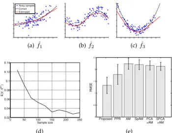
Fig. 1. (a) to (c): Transfer functions estimated using our approach (solid red line) and ground truth (dashed black line). The blue dots represent noisy samples used to train the model(n = 100). (d) Weight matrix errorE(V,VGT)as function of the sample sizen. (e) RMSE between
estimated signal and testing signal generated according to Eq.(7), for the different approaches. The results of experiments (d) and (e) are averaged over300trials.
Besides these performance measures, we also report the “complexity” of the different methods, which is measured by the number of learned functions. We finally report the sparsity of the weight matrixV.
4.3 TOY EXAMPLE
In our first experiment, we generate n samples using the following additive model
yi=f1(0.5xi,1+ 0.25xi,2+ 0.25xi,3) +f2(xi,4)
+f3(0.5xi,5+ 0.5xi,6) +i, (7) where f1(x) = 2 exp(x), f2(x) = 2 sin(πx), f3(x) = 10x2,
the error terms i are iid samples from a standard normal distribution, and the covariates x1, . . . , x6 are iid samples
from a uniform distribution on[−1,1]. For our method,G is set as the trivial group {1, . . . ,6} (i.e. constraint(C1) is not used here as we allow for any combination of thep= 6 features) andr=r1 = 3. We fix the number of iterations of
our method toN = 20.
Figure 1 (a-c) shows the estimated transfer functions using our proposed method for a sample of sizen = 100, together with the true transfer functions. As can be seen, our method yields good approximations of the true transfer functions, despite the relatively small sample size. We then evaluate the ability of the algorithm to estimate the true weight matrixV. Figure 1(d) shows the metricE(V,VGT) depending on the number of samples n. For low n, the error is relatively high (about the same order as the entries in VGT). As the sample size increases, the error becomes one order of magnitude lower than the entries of VGT. Finally, we evaluate the RMSE on a test set of n = 100 samples generated according to Eq. (7). Figure 1(e) shows that our approach yields a lower RMSE than AM (learned with 6 transfer functions, one per covariate), PPR, SpAM, as well as unsupervised dimensionality reduction techniques (PCA+AM and SPCA+AM) with3derived covariates. Note
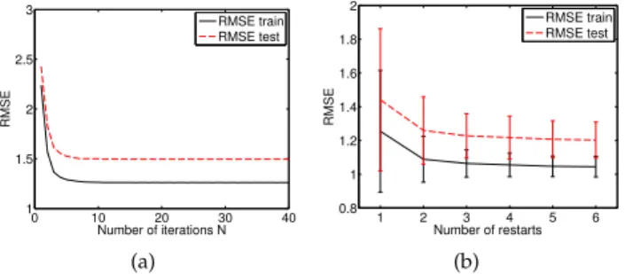
0 10 20 30 40 1 1.5 2 2.5 3 Number of iterations N RMSE RMSE train RMSE test (a) 1 2 3 4 5 6 0.8 1 1.2 1.4 1.6 1.8 2 Number of restarts RMSE RMSE train RMSE test (b)
Fig. 2. Training and testing RMSE versus number of iterations N (left), and number of restarts (right) for the example in Sec. 4.3. The results are averaged over50trials.
that our approach yields a better performance than less con-strained models (e.g., PPR) as the introduced constraints act as a regularizer that prevents overfitting, and significantly reduce the model complexity.
We now examine the influence of the number of itera-tionsN on the performance of SDRAM. Figure 2(a) shows the training and testing RMSE with respect toN. After a few iterations, the algorithm reaches a stable solution. Setting N = 20 is therefore a conservative choice that we use in all experiments. Moreover, similarly to any nonconvex procedure, our algorithm is sensitive to initialization. To further evaluate this point, we illustrate in Fig. 2(b) the training and testing RMSE with respect to the number of restarts of SDRAM (for each restart, SDRAM is initialized randomly, and the instance yielding the lowest training RMSE is selected). It can be seen that using multiple restarts improves the performance of SDRAM on this example; we set the number of restarts to3in the following experiments. 4.4 SHARED BICYCLE SYSTEM DATA
In our second experiment, we consider a real-world regres-sion problem: predicting the number of available bikes in the shared bicycle system of Dublin, Ireland. More specifi-cally, the goal is to provide one-hour ahead forecasts of bike availability for all44 bicycle stations across the city, using as inputs weather data, calendar information (e.g., weekday, hour of the day) and the lagged number of available bikes at all stations. A key challenge is to effectively capture correlations of bike availability across different stations and incorporate those into the predictions.
The dataset contains the number of available bikes for all 44bike stations in the city of Dublin4, at a sampling rate of5 minutes, over a time period of351days. We use the first200 days for training and the remaining151days for testing. We consider the input variables “Time of Day”, “Day of Week” and “Temperature”, as well as the number of available bikes at all44stations one hour before prediction, hencep= 47 in this experiment. We induce the following groups
G={{“Time of Day”},{“Temperature”}, {“Day of Week”},{“Lagged availability”}}, and use our algorithm to derive two covariates from the “Lagged availability” group (i.e., we setr1=r2 =r3 = 1,
4.http://www.dublinbikes.ie
andr4= 2). We set the smoothing and ridge regularization
parameters equal toλ = ν = 1. Using cross-validation to optimize these parameter values is likely to improve the accuracy, but comes at extra computational costs.
We denote by AM1 and AM2 two additive models where AM1 uses allp = 47input variables as covariates, while AM2 only uses 4 covariates, namely “Time of Day, “Temperature”, “Day of Week” and “Lagged availability at the station to predict”. In other words, AM2 ignores the number of available bikes at other stations. Table 1 provides a comparison of the different methods in terms of performance and model complexity, measured by the number of learned transfer functions. While PPR outper-forms SDRAM on the training set, its performance is worse on the testing set. Confirming the findings inZhang et al.
(2008), this result suggests that, without imposing any con-straints, PPR tends to overfit the data. Note that SDRAM also outperforms AM1 and AM2 on the testing set. While AM2 provides an average testing accuracy close to SDRAM, it handles the stations independently and therefore does not provide insights into correlations among different stations. Moreover, our approach compares favorably to SpAM, even if SDRAM learns much less functions. SDRAM also sig-nificantly outperforms unsupervised dimensionality reduc-tion approaches PCA+AM, and SPCA+AM5. The paired Wilcoxon test shows that the improvement of SDRAM over all these methods is statistically significant at a significance level of0.01. We also compared SDRAM with SDRAM-C2, a variant of the proposed approach where only constraint (C2) is active (i.e., we set L = 1 for (C1) and (C3) is ignored). SDRAM-C2 can be seen as a variant of Sparse PPR (Zhang et al.,2008), where the`1norm of the weights
is used as a regularizer to achieve weight sparsity. Table 1 shows that SDRAM-C2 achieves comparable accuracy with SDRAM6. Despite not having a direct impact on the accuracy on this task, constraints (C1) and (C3) are nevertheless crucial to obtain an interpretable model. To illustrate this point, Figure 3 displays the weight matrices obtained using SDRAM, PPR, PCA+AM and SDRAM-C2 for one particular bike station (Station 1). While competing methods yield adenseandunstructuredmatrix, the solution of SDRAM isstructuredandsparse. Quantitatively, SDRAM yields for this station a weight matrix with83%zero entries, while the matrices obtained via PPR and PCA methods are fully dense, and SDRAM-C2 provides a matrix with 20% zeros. More importantly, PPR, PCA and SDRAM-C2 provide unstructured weight matrices that combine inputs of different physical types, e.g., temperature, time of day and number of available bicycles; this makes it virtually impossible to interpret the relations between inputs and outputs in a meaningful way. Conversely, our method keeps variables of different physical types separated. To highlight the interpretability of the obtained solution, Fig. 4 shows maps with the estimated weights given to the lagged input variables for the two derived covariates, along with the
5. The results for SPCA+AM are not reported in the Table 1, as the best accuracy for this experiment is reached when the sparsity
parameter is equal top= 47, which is equivalent to PCA+AM.
6. The difference of testing average RMSE between SDRAM and SDRAM-C2 in Table 1 isnotstatistically significant using the Wilcoxon test.
TABLE 1
Average RMSE on training and testing sets, average number of learned functions and average number of non-zero elements inVover44stations. The symbol∗indicates testing RMSEs that are significantly higher than the ones obtained by SDRAM, at a significance level of0.01.
Method RMSE Complexity
Training Testing # functions Vsparsity
SDRAM 3.21 3.21 5 79%
PPR 3.07 3.31∗ 5 0%
Additive models AM1 3.05 3.34∗ 47 NA
AM2 3.38 3.26∗
4 NA
SpAM 3.25 3.28∗ 38.4 NA
PCA + AM 5.20 5.32∗ 5 0%
SDRAM-C2 3.02 3.16 5 20%
Fig. 3. Weight matrix V learned using SDRAM, PPR, PCA, and SDRAM-C2. Thexaxis denotes the derived variable number, and they
axis is the input variable number. The first three input variables are “Time of Day”, “Temperature” and “Day of Week”. The remaining44variables are the lagged variables.
associated transfer functions. In these maps, the station to predict (Station 1) is denoted with a big dot. While the first transfer function represents a positive correlation between the number of available bikes at time t −1h and at t, the second transfer function shows a negative correlation. Interestingly, one can see that the first derived variable essentially corresponds to the lagged number of available bikes at the station to predict (Station 1). On the other hand, the second derived variable combines several stations that are negatively correlated with the response variable. Note that this intuitive separation of the covariates is essentially due to the disjoint support constraint(C3)which allows to disentangle positive and negatively correlated stations. To further show this point, Fig. 5 shows the estimated maps when constraint (C3) is not active. Unlike in Fig. 4, some stations are active in both maps (e.g., see the station repre-sented with a big dot that is maximally active in both cases). This results in entangled positive and negative correlation effects for each station, which leads to a very difficult inter-pretation as cancellations systematically occur between the different transfer functions. On the other hand the obtained maps in Fig. 4 can be readily interpreted: the bike station for which the predictions are computed lies in the commercial
0.1 0.2 0.3 0.4 0.5 −1 −0.5 0 0.5 1 −10 −5 0 5 10 15 20 25 0 0.05 0.1 0.15 −1 −0.5 0 0.5 1 −4 −2 0 2 4 6 8 10
Fig. 4. Public bike availability forecasting: weights learned with SDRAM for the first and second derived covariate, shown on a map of Dublin with the 44 stations. The big dot denotes the station where prediction occurs. The shape of the corresponding transfer function is shown in the top left corner of each map.
Fig. 5. Weights learned using our methodwithout imposing constraint
C3. Note that some stations are active in both maps. For example, the station where the prediction occurs (represented by a big dot) is the maximally active station in both maps.
heart of the city and close to important transportation hubs. The negative correlation is due to the mobility patterns of Dublin commuters: the three top weighted stations are Smithfield North, Pearse and Leinster Street. The first one is located in a residential area and the latter two are on a university campus. In mornings and evenings, people commute by bike from their homes in the residential area to their working places in the city center. In addition, students pick up bikes at this tranportation hub to complete the last mile of their journey to the university campus.
4.5 ELECTRIC LOAD FORECASTING
In our last experiment, we apply our algorithm to short-term electric load forecasting. Note that additive models have been quite successfully applied to this task previously, with covariates including calendar information, weather data as well as auto-regressive and lagged features (Fan and Hyndman,2012). A difficult problem is how to optimally incorporate localized weather measurements, i.e., how to weight the input from weather stations in different regions in order to predict electric load at the state level. The authors of (Goude et al.,2014) state this as an open problem and explicitely mention the need for automatic covariate selection methods. In (Ba et al.,2012), weather stations are weighted according to the relative load in that particular region. Similarly, one could consider socio-economic indica-tors (population density, type of heating in different parts of the state, etc), however this information is not always available. Our solution is to simulateously learn the weights and transfer functions from the data.
The dataset comes from two sources: hourly electric load data for the state of Vermont, USA, from ISO New Eng-land7 and temperature data from 40 weather stations from MADIS8. The prediction task is to forecast electrical loads 24 hours ahead of time. The input variables in our model are “Time of Year”, “Time of Day”, “Day of Week”, “Lag load” and “T”, i.e., the temperatures from the 40 weather stations. Similarly to the model in (Fan and Hyndman,2012), we also consider “Tlag24” (the temperatures from the 40 weather
stations lagged by 24 hours), “Tmean24”, “Tmin24”, “Tmax24”
(the mean, minimum and maximum over the past 24 hours
7.http://www.iso-ne.com/isoexpress/web/reports/ load-and-demand/-/tree/dmnd 8.http://madis.noaa.gov/ 2 4 6 8 10 20 40 60 80
Number of derived covariates
R M S E Training Testing
Fig. 6. RMSE of the PPR method as a function of the number of derived covariates.
for each station) and “Tmean7” (the mean over the past seven
days for each station). We enforce the following groups in the derivation of the covariates
G={{“Time of Year”},{“Time of Day”}, {“Day of Week”},{“Lag load”},{T}, {Tlag24},{Tmean24},{Tmin24},
{Tmax24},{Tmean7}},
and derive one variable per group in our method (i.e., we set rl = 1 for l ∈ [10]). The dataset is split as follows: omitting any time points for which we have missing load or temperature values, we use 9013 observations between 4 January, 2011 and 31 December, 2012 for training, and 4149 observations between 1 January, 2013 and 31 January, 2014 for testing.
We denote by AM1-3 the three additive models defined as follows. AM1 learns one transfer function for each of the 244 input variables. AM2 and AM3 learn one transfer function for each of the 10 groups, where AM2 uses the average of the 40 temperature inputs as covariates, and AM3 selects the inputs from the city of Burlington, which is the area with the highest population density in Vermont.
Table 2 shows that SDRAM provides the best perfor-mance: it has the lowest testing RMSE, a limited number of transfer functions, and provides a sparse dimensionality reduction matrix. The second lowest testing RMSE is ob-tained by SpAM. However, 1) SpAM learns approximately 8 times more functions than than SDRAM and 2) SpAM acts as a feature selection algorithm, and does not derive covariates out of existing input variables. Note also that the proposed method compares favorably to SDRAM-C2, which only considers constraint (C2). It should be noted moreover that SDRAM-C2 systematically yields derived co-variates that combine input variables with different physical units, leading to a loss of interpretability. Moreover, input variables take part in many derived covariates as(C3)is not active, which makes it difficult to track the effect of input variables on the response variable. AM1 and PPR methods suffer from overfitting as they provide good training accu-racy but do not generalize well on the test set. To further study this behaviour, we evaluated the testing accuracy of PPR as a function of the number of derived covariates (see Fig. 6). We have observed that PPR strongly overfits the data whenr ≥ 3, leading to very poor testing accuracy. Hence,
TABLE 2
Model accuracy (RMSE) and complexity on the electric load forecasting problem.
Method RMSE Complexity
Training Testing # functions Vsparsity
SDRAM 26.6 27.6 10 98%
PPR r= 1 35.8 45.8 1 0%
r= 2 31.9 44.2 2 0%
r= 10 16.7 72.5 10 0%
Additive models AM1 24.4 28.3 244 NA
AM2 28.1 28.8 10 NA AM3 27.9 28.5 10 NA SpAM 26.0 28.1 78 NA PCA + AM r= 10 39.2 39.7 10 0% r= 100 34.6 40.8 100 0% SPCA + AM r= 10 28.7 31.2 10 96% r= 100 27.1 29.6 100 96% SDRAM-C2 26.3 28.3 10 9.1%
the constraints onVare crucial to avoid overfitting. As for PCA + AM and SPCA + AM, it can be noted that these unsupervised dimensionality reduction approaches provide significantly lower accuracy than SDRAM.
To further study the interpretability of the obtained solution, Fig. 7 shows the maps of the weights associated with the different weather stations in the derivation of the temperature-related covariates. Interestingly, for most derived covariates, our algorithm selects stations in the Burlington area, which has the highest population density in Vermont. Moreover, there is also a representative selection of stations in the Western/Eastern part of Vermont, which have warmer/colder climate, respectively9.
5
CONCLUSION
We proposed a novel framework for learning additive mod-els with a moderate number of covariates derived from a potentially large set of input variables. Our approach allows for the representation of structure in the input variables, which helps to prevent overfitting and leads to models that provide practical insights into relations between inputs and output. We established identifiability of the proposed model under mild assumptions on the transfer functions. We de-rived an efficient learning algorithm that alternates between a regularized least squares problem and a mixed-integer problem. We conducted experiments on synthetic and real-world data; the results showed that SDRAM outperforms baseline methods and highlighted the importance of the proposed contraints. Our work significantly broadens the applicability of additive models to high-dimensional prob-lems while maintaining their interpretability and potential to provide practical insights.
9.http://www.nws.noaa.gov/climate/local data.php?wfo=BTV, see Vermont Annual Mean High/Low Temperature
Acknowledgments.The authors would like to thank the associate editor and the anonymous reviewers for their valuable com-ments and references that helped to improve the quality of this paper.
APPENDIX
A
PROOF OF
THEOREM
2.2
A.1 Preliminary resultsOur proof relies on a number of results that we give in this sec-tion. To start with, the following result establishes identifiability when we have only one ridge function.
Proposition A.1. Suppose thatfandhare functions (not identically zero) such thatf(0) =h(0) = 0. Assume that
∀x∈Rp, f(vTx) =h(wTx), (8)
withvandwnon-negative vectors with unit`1norm. Thenv=w,
andf=h.
Proof. We proceed by contradiction, and assume that v and
w are not collinear. In other words, assume that span(v) 6=
span(w), which is equivalent tospan(v)⊥ 6= span(w)⊥.
More-over, span(v)⊥ is not strictly included in span(w)⊥, as both
subspaces have the same dimension. Therefore, there exists
x0 such that x0 ⊥ v and x0 ∈/ span(w)⊥. In other words,
vTx0= 0, andwTx06= 0. For anyµ∈R, we therefore have
f(vT(µx0)) =f(µvTx0) =f(0) = 0 =h(wT(µx0)) =h(µwTx0 | {z } 6 =0 ). (9)
We therefore obtainh(z) = 0for allz, which contradicts our
assumption. Hence, we conclude thatv = λwfor some
non-negative real value λ. Since kvk1 = kwk1, we therefore get
λ= 1, andv=w. Hence,f=h.
Using this result, we establish identifiability when ridge functions are quadratic
−76 −74 −72 −70 42 43 44 45 46 0.05 0.1 0.15 0.2 0.25 0.3 (a)T −76 −74 −72 −70 42 43 44 45 46 0.05 0.1 0.15 0.2 0.25 0.3 (b)Tlag24 −76 −74 −72 −70 42 43 44 45 46 0.1 0.2 0.3 0.4 0.5 0.6 (c)Tmean24 −76 −74 −72 −70 42 43 44 45 46 0.1 0.2 0.3 0.4 0.5 (d)Tmin24 −76 −74 −72 −70 42 43 44 45 46 0.05 0.1 0.15 0.2 0.25 (e)Tmax24 −76 −74 −72 −70 42 43 44 45 46 0.2 0.4 0.6 0.8 (f)Tmean7
Fig. 7. Electric load forecasting: weights learned by SDRAM for the various temperature-based covariates, shown on a map of Vermont with the40
temperature stations.
Proposition A.2. Let{vj}rj=1and{wj}sj=1be weight vectors that
satisfy constraints(C1),(C2)and(C3). Suppose that
∀x∈Rp, r X j=1 fj(vTjx) = s X j=1 hj(wjTx), (10)
where {fj}rj=1 and {hj}sj=1 are quadratic functions with at most
one linear function. We assume moreover that the functions are not identically zero and satisfyfj(0) = hj(0) = 0. Then,r = s and
there exists a permutationπsuch that, for allj∈[r]
vj=wπ(j), fj=hπ(j). (11)
Proof. Notice first that in order to prove identifiability in this case, it is sufficient to prove the following statement
∀j∈[r], ∃π(j)such that supp(vj) =supp(wπ(j)). (12)
Indeed, if Eq. (12) holds, then by evaluating Eq. (10) atxsuch
that supp(x) =supp(vj), we get
fj(vTjx) =hπ(j)(w
T
π(j)x),
where we used the disjoint supports assumption and the fact
thatfj(0) =hk(0) = 0for allj, k. The above equality
general-izes to anyxinRpasvjandwπ(j)have zero entries outside of
supp(vj)
∀x∈Rp, fj(vjTx) =hπ(j)(w
T
π(j)x). (13)
We therefore obtain from Proposition A.1 thatvj=wπ(j)and
fj=hπ(j). Note moreover thatπis one-to-one asπ(j1) =π(j2)
would imply supp(vj1) = supp(vj2) which contradicts the
disjoint support assumption. We therefore getr=s.
We now focus on proving Eq. (12). To do that, assuming the functions are quadratic, the main idea is to look at the
monomials of degree2(i.e., of the formxaxb) in Eq. (10). The
equality of the monomials in Eq. (10) imposesS
jsupp(vj)×
supp(vj) =Sjsupp(wj)×supp(wj), from which we can see
that the supports of vj and wj have to be the same (up to
a permutation), due to the disjoint support constraint. More formally, let us proceed by contradiction and assume that Eq.
(12) does not hold. There existsj0for which
∀j∈[s], supp(vj0)6=supp(wj). (14) Then, ∀x∈Rp supp(x) =supp(vj0) , fj0(v T j0x) = s X j=1 hj(wTjx). (15)
We first examine the case where fj0 is linear. If this holds,
then the right hand side of Eq. (15) also has to be linear. Since there is at most one linear function, the above equality
becomesavT
j0x=bw
T
j1xfor allxwith the same support asvj0,
for some a, b, and index j1. If supp(vj0) 6⊂ supp(wj1), then
there exists k such that vj0k 6= 0 and wj1k = 0. By setting
x = ek, we get avj0k = 0, and therefore a = 0. Since the
functions are not identically zero, this cannot hold and we have
supp(vj0)⊂supp(wj1). In that case, we havebw
T
j1x=av
T
j0x
for allxsuch that supp(x) =supp(wj1), and we obtainb= 0
for the same reasons above. Therefore,fj0cannot be linear.
Let us now examine the case wherefj0 is a quadratic
(non-linear) function. Assume first that supp(vj0) 6⊂supp(wj) for
allj. If Eq. (15) is to hold, there exists at least onejsuch that
supp(vj0)∩supp(wj)6=∅, and letj1be such an index. Denote
supp(wj1) there exists an element l ∈ supp(vj0) and not in
supp(wj1). Therefore, the cross-termxkxl belongs to the left
hand side of Eq. (15), but not to the right hand side. This cannot
hold, and we conclude that there exists an element j1 such
that supp(vj0) ⊂supp(wj1). Note that we havehj1(w
T
j1x) =
P
jfj(v
T
jx) for all x such that supp(x) = supp(wj1). As
before, there exists an element k ∈ supp(vj0)∩supp(wj1),
andl∈supp(wj1), butl /∈supp(vj0). Therefore, the previous
equality has the cross-term xkxl on the left hand side, but
not on the right hand side. This concludes the proof of the proposition.
In order to extend our proof from quadratic ridge functions to general continuous functions in Section A.2, we rely on the
following result fromKhatri and Rao(1968).
Lemma A.3. Consider the functional equation
φ1(αT1t) +· · ·+φr(αTrt) =ξ1(t1) +· · ·+ξp(tp)
defined for |ti| ≤ δ, i = 1, . . . , p, whereδ > 0, t represents the
column vector of variablest1, . . . tp, andα1, . . . ,αrare the column
vectors of ap×rmatrixA. LetAbe of full column rank such that each column has at least two non-zero entries. Then,φ1, . . . , φr and
ξ1, . . . , ξpare all quadratic functions.
A.2 Proof of Theorem 2.2
Let us note F , {f: R → R ; fcontinuous, f(0) =
0andfis not identically zero}. Let us assume{(fj,vj)∈ F ×
Rp}1≤j≤rand{(hj,wj)∈ F ×Rp}1≤j≤sare such that
(Hr) : r, s≤p , ∀x∈Rp, µ+Prj=1fj(v T jx) =ν+ Ps j=1hj(w T jx),
{vj}1≤j≤rsatisfy the constraints(C1),(C2)and(C3),
{wj}1≤j≤ssatisfy the constraints(C1),(C2)and(C3),
At most onefj(and onehj) is linear.
First, usingx= 0givesµ=ν.
Without loss of generality, we also assume r ≤ s. We
proceed by induction onrto show that the following property
(Pr) : (Hr)implies identifiability
holds for allr.
A.2.0.1 Initialization (r = 1): First we complete the
set of orthogonal vectors{wj}1≤j≤s in an orthogonal basis of
Rpand noteW ,(w1, . . . ,wp). We also defineuj ,W−1vj
for1≤j≤r. We have ∀x∈Rp, f1(vT1x) = s X j=1 hj(wTjx), (16) ∀x∈Rp, f1(uT1WTx) = s X j=1 hj(eTjWTx), (17)
where ej is the vector with all zero elements, except thejth
element is equal to one.
Now we do the change of variablez=WTxand obtain
∀z∈Rp, f1(uT1z) = s X j=1 hj(zj). (18) Settingz=zkek, we get For1≤k≤s: ∀zk∈R, f1(u1kzk) =hk(zk), (19) Fors < k≤p: ∀zk∈R, f1(u1kzk) = 0. (20)
Note that ifu1k = 0for some1≤k≤s, then using equation
(19) would imply thathk= 0, which is impossible sincehk∈ F.
Also, if u1k 6= 0 for some s < k ≤ p, then using equation
(20) would implyf1 = 0, which is impossible sincef1 ∈ F.
So we haveu1 = (u11, ..., u1s,0, . . . ,0)with u11, . . . , u1s 6= 0.
Assumings > 1, we takez= (z1, z2,0, . . . ,0) and using (18)
and (19) we get
∀z1, z2∈R, f1(u11z1+u12z2) =h1(z1) +h2(z2)
=f1(u11z1) +f1(u12z2).
(21)
Thereforef1 satisfies Cauchy’s functional equation, so it isQ
-linear. Since it is also continuous,f1is (R-)linear, and by (19) so
areh1 andh2. This is impossible, sos = 1 =r. Therefore we
haveu1=λe1and (18) becomes
∀z1∈R, f1(λz1) =h1(z1). (22)
We also get v1 = Wu1 = λWe1 = λw1. Since kv1k1 =
kw1k1 = 1, we getλ=±1. The positivity ofv1 andw1 gives
λ= 1, and thusv1 =w1andf1=h1.
A.2.0.2 Induction: Now let us assume the hypotheses
(Hr+1) and (Pr) hold. The strategy is to show thatfr+1 =hs
andvr+1 = ws (up to a permutation of the terms), and (Hr)
holds. Calling (Pr) would then terminate the proof of (Pr+1).
The same change of variable as in the initialization gives
∀z∈Rp, r+1 X j=1 fj(uTjz) = s X j=1 hj(zj). (23)
First case: all{uj}1≤j≤r+1 have at least two non-zero
en-tries. Then, using Lemma A.3, all ridge functions are quadratic. If the ridge functions contain at most one linear function, our model is identifiable according to Proposition A.2. Otherwise, the assumption is not satisfied.
Second case: there exists oneuj with one non-zero entry.
Without loss of generality, let us say thisujisur+1, and with
a permutation of coordinates take ur+1 = λes, for some λ.
Using the equalityvr+1 =Wur+1 =λws and the unit norm
constraints onvr+1,wswe getλ= 1. We therefore haveur+1=
es, andvr+1=ws. Note also that
∀j∈[r], vTjvr+1=vjTws= (Wuj)Tws
=uTjeskwsk22
=ujskwsk22, (24)
where we have used the fact that the columns of W are
orthogonal. Since thevjs are orthogonal to each other, we have
vT
jvr+1 = 0, and thereforeujs = 0for allj ∈ [r]as ws is a
nonzero vector. By rewriting Eq. (23) and setting zs = 0, we
have ∀z∈Rp zs= 0 , r X j=1 fj(uTjz) = s−1 X j=1 hj(zj), (25)
Moreover, sinceujs = 0for allj ∈ [r], the above equality is
valid for allz∈Rp, and we have
∀z∈Rp, r X j=1 fj(uTjz) = s−1 X j=1 hj(zj). (26) Using the change of variables, we therefore get
∀x∈Rp, r X j=1 fj vjTx = s−1 X j=1 hj(wTjx). (27)
which corresponds to (Hr). By calling (Pr), we haver =s−1
and there exists a permutationπ: [r]→[r]such that
∀j∈[r], fj=hπ(j), vj=wπ(j). (28)
We therefore have fr+1(vTr+1x) = hs(wTsx), and using the
equality vr+1 = ws, we conclude that fr+1 = hs. (Pr+1)
A.3 Tightness of the condition in Theorem 2.2
We give the following counter-example to show that the as-sumption requiring at most one linear transfer function is necessary ∀x∈R3, 1 2 1 0 0 x + 0 12 12 x = 1 2 1 2 0 x +1 2 0 0 1 x . (29) The above model is unidentifiable as the left-hand side and
right hand side models are equal for allx∈R3, yet the model
parameters are different. Note also that the weight vectors in the above example are admissible as they satisfy the constraints of our model.
We finally highlight the fact that, unlike the general (un-constrained) PPR model where identifiability does not hold
for quadratic transfer functions Yuan (2011), the proposed
(constrained) model is identifiable in that case.
APPENDIX
B
DERIVATION OF THE OBJECTIVE FUNCTION
LIN-EARIZATIONIn this section, we give the derivations used in our optimization algorithm in detail. Recall that our regression problem is given as follows (P): min β∈R(kr),V∈V ky−S(V)βk22+λβ T Cβ+νβTβ.
We focus on solving (P) forVwith a fixedβ. We linearize the
functionsst(vTjxi)aroundv0j st(vTjxi)≈st((v0j) T xi) + (vj−v0j) T∇ vst(vTxi) v=v0 j =st((v0j) T xi) + (vj−v0j) T xis0t((v 0 j) T xi).
Plugging this approximation inSj(vj), we get
Sj(vj) = s1(vTjx1) . . . sk(vjTx1) s1(vTjx2) . . . sk(vjTx2) .. . ... ... s1(vTjxn) . . . sk(vTjxn) ≈Sj(v0j) + (vj−v0j)Tx1s01((v0j)Tx1) . . . (vj−v0j)Tx1s0k((v0j)Tx1) .. . ... ... (vj−v0j)Txns01((v0j)Txn) . . . (vj−vj0)Txns0k((v0j)Txn) =Sj(v0j) +S 0 j(v 0 j)((X(vj−v0j))11×k) ,Sj(vj0) + ˜Sj(vj),
where denotes the point wise matrix operation, the data
matrixX= x1 x2 · · · xn T ∈Rn×p, and S0j(v 0 j) = s01((v0j)Tx1) . . . s0k((v0j)Tx1) .. . ... ... s01((vj0)Txn) . . . s0k((v 0 j)Txn) ∈R n×k . We therefore obtain S(V)≈S(V0) + ˜S(V),
whereS˜(V)is obtained by concatenating the differentS˜j(vj).
Then, we have S(V)β ≈ S(V0)β+Pr
j=1S˜j(vj)βj, where
βjdenotes the vector of lengthk whose entries represent the
coefficients of thejth transfer function. Note that for anyj, we
have ˜ Sj(vj)βj= βj1In×n· · · βjkIn×n vec(˜Sj(vj)) = βj1In×n · · · βjkIn×n · vec(S0j(v 0 j))11×p (1k×1⊗X) (vj−v0j) ,Mj(vj−v0j),
with⊗denoting the Kronecker product. Therefore, settingM
to be equal to[M1|. . .|Mr], we get r X j=1 ˜ Sj(vj)βj=− r X j=1 Mjv0j+ r X j=1 Mjvj =−Mvec(V0) +Mvec(V) ,b+Mvec(V).
Finally, we solve the following approximate problem, whenβ
is fixed, min V∈V ky˜−Mvec(V)k 2 2, wherey˜=y−S(V0)β−b.
REFERENCES
Ba, A., Sinn, M., Goude, Y., and Pompey, P. (2012). Adaptive learning of smoothing functions: application to electricity
load forecasting. InAdvances in Neural Information Processing
Systems (NIPS), pages 2519–2527.
Chen, Y. and Samworth, R. (2014). Generalised additive
and index models with shape constraints. arXiv preprint
arXiv:1404.2957.
Fan, S. and Hyndman, R. J. (2012). Short-term load forecasting
based on a semi-parametric additive model. IEEE
Transac-tions on Power Systems, 27(1):134–141.
Friedman, J. H. and Stuetzle, W. (1981). Projection pursuit
re-gression.Journal of the American Statistical Association, 76:817–
823.
Goude, Y., Nedellec, R., and Kong, N. (2014). Local short and middle term electricity load forecasting with semi-parametric
additive models. IEEE Transactions on Smart Grid, 5(1):440–
446.
Guyon, I. and Elisseeff, A. (2003). An introduction to variable
and feature selection. Journal of Machine Learning Research,
3:1157–1182.
Hastie, T., Tibshirani, R., and Friedman, J. (2009). The elements
of statistical learning, volume 2. Springer.
Hastie, T. J. and Tibshirani, R. J. (1990). Generalized additive
models, volume 43. CRC Press.
Hu, J., Mitchell, J., Pang, J.-S., Bennett, K., and Kunapuli, G. (2008). On the global solution of linear programs with linear
complementarity constraints. SIAM Journal on Optimization,
19(1):445–471.
Huang, J., Horowitz, J. L., and Wei, F. (2010). Variable selection
in nonparametric additive models. The Annals of Statistics,
38(4):2282.
Jeroslow, R. (1978). Cutting planes for complementarity
con-straints. SIAM Journal on Control and Optimization, 16:56–62.
Jolliffe, I. (2005). Principal component analysis. Wiley Online
Library.
Khatri, C. and Rao, C. R. (1968). Solutions to some functional equations and their applications to characterization of
prob-ability distributions. Sankhy¯a: The Indian Journal of Statistics,
Series A, pages 167–180.
Lee, D. D. and Seung, H. S. (1999). Learning the parts of objects
by non-negative matrix factorization. Nature, 401(6755):788–
791.
Morton, S. C. (1989).Interpretable projection pursuit. PhD Thesis,
Peng, R. D. and Welty, L. J. (2004). The NMMAPSdata package.
R News, 4(2):10–14.
Ravikumar, P., Lafferty, J., Liu, H., and Wasserman, L. (2009).
Sparse additive models.Journal of the Royal Statistical Society:
Series B (Statistical Methodology), 71(5):1009–1030.
Sj ¨ostrand, K., Clemmensen, L. H., Larsen, R., and Ersbøll,
B. (2012). Spasm: A matlab toolbox for sparse statistical
modeling.Journal of Statistical Software Accepted for publication.
Su, L. and Zhang, Y. (2013). Variable selection in nonparametric
and semiparametric regression models. InHandbook in
Ap-plied Nonparametric and Semi-Nonparametric Econometrics and Statistics. Oxford University Press.
van der Maaten, L. J., Postma, E. O., and van den Herik, H. J.
(2009). Dimensionality reduction: A comparative review.
Journal of Machine Learning Research, 10(1-41):66–71.
Wang, X. and Brown, D. (2011). The spatio-temporal
gen-eralized additive model for criminal incidents. In IEEE
International Conference on Intelligence and Security Informatics (ISI), pages 42–47.
Wolsey, L. (1998).Integer Programming. Wiley Series in Discrete
Mathematics and Optimization. Wiley.
Wood, S. (2006).Generalized additive models: an introduction with
R. CRC press.
Yuan, M. (2011). On the identifiability of additive index models.
Statistica Sinica, 21(4):1901.
Zhang, X., Liang, L., Tang, X., and Shum, H.-Y. (2008). L1 regularized projection pursuit for additive model learning. In IEEE conference on computer vision and pattern recognition (CVPR), pages 1–8.
Zhao, T. and Liu, H. (2012). Sparse additive machine. In
International Conference on Artificial Intelligence and Statistics (AISTATS), pages 1435–1443.
Zhu, X., Huang, Z., Shen, H. T., Cheng, J., and Xu, C. (2012). Dimensionality reduction by mixed kernel canonical
correla-tion analysis.Pattern Recognition, 45(8):3003–3016.
Zhu, X., Huang, Z., Yang, Y., Shen, H. T., Xu, C., and Luo, J. (2013). Self-taught dimensionality reduction on the
high-dimensional small-sized data. Pattern Recognition, 46(1):215–
229.
Zhu, X., Suk, H.-I., and Shen, D. (2014). Matrix-similarity based loss function and feature selection for alzheimer’s disease
diagnosis. InIEEE Conference on Computer Vision and Pattern
Recognition (CVPR), pages 3089–3096. IEEE.
Zou, H., Hastie, T., and Tibshirani, R. (2006). Sparse principal
component analysis. Journal of computational and graphical
statistics, 15(2):265–286.
Alhussein Fawzireceived the M.Sc. degree in electrical and electronics engineering from the Swiss Federal Institute of Technology (EPFL), Lausanne, Switzerland in 2012. He is currently pursuing the PhD degree with the Signal Pro-cessing Laboratory (LTS4) at EPFL. His re-search interests include sparse signal and image processing, data mining and machine learning. He received twice the IBM PhD fellowship, in 2013 and 2015.
Jean-Baptiste Fiot is a Research Scientist at IBM Research - Ireland since December 2013. He received a Ph.D. degree in Applied Mathe-matics in 2013 from Paris Dauphine University in France, a Master degree in Applied Mathe-matics in 2009 from Ecole Nationale Superieure de Cachan in France, and a Master degree in Engineering in 2009 from Ecole Centrale Paris in France. Before joining IBM, he held Research positions in Paris Dauphine University in France, in Samsung Advanced Institute of Technology (SAIT) in South Korea, and in CSIRO - Australian e-Health Research Centre (AeHRC) in Australia. He was awarded the Best Student Paper Award in the VIPIMAGE 2011 conference, and the Thesis Prize 2014 of the Dauphine Foundation. His research interests include machine learning, signal and image processing, and optimization.
Bei Chen is a Research Staff Member in the Big Data Analytics & Systems department. She received her Ph.D. in Statistics from the Univer-sity of Waterloo. Her current research interests include time series analysis, forecasting, resam-pling methods for dependent data and financial econometrics. Dr. Chen has more than 20 ref-ereed publications in journals and international conferences.
Mathieu Sinnis a Research Staff Member and Manager in the Big Data Analytics & Systems department at the IBM Research laboratory in Dublin, Ireland. He received a Diploma in com-puter science in 2006, and a Ph.D. degree in mathematics in 2009, both from the University of Lbeck, Germany. Subsequently he was a Post-doctoral Research Fellow at the University of Waterloo, Canada, before joining IBM Research in 2011. His research interests lie at the inter-section of statistics, machine learning and the analysis of real-world time series data. Dr. Sinn is the author or coauthor of 4 patents and more than 40 technical papers.
Pascal Frossard(S96,M01,SM04) received the M.S. and Ph.D. degrees, both in electrical en-gineering, from the Swiss Federal Institute of Technology (EPFL), Lausanne, Switzerland, in 1997 and 2000, respectively. Between 2001 and 2003, he was a member of the research staff at the IBM T. J. Watson Research Center, Yorktown Heights, NY, where he worked on media coding and streaming technologies. Since 2003, he has been a faculty at EPFL, where he heads the Sig-nal Processing Laboratory (LTS4). His research interests include graph signal processing, image representation and coding, visual information analysis, and distributed signal processing and communications.
Dr. Frossard has been the General Chair of IEEE ICME 2002 and Packet Video 2007. He has been the Technical Program Chair of IEEE ICIP 2014 and EUSIPCO 2008, and a member of the organizing or technical program committees of numerous conferences. He has been an Associate Editor of the IEEE TRANSACTIONS ON SIGNAL PROCESSING ), IEEE TRANSACTIONS ON BIG DATA (2015-), IEEE TRANSACTIONS ON IMAGE PROCESSING (2010-2013(2015-), the IEEE TRANSACTIONS ON MULTIMEDIA (2004-2012), and the IEEE TRANSACTIONS ON CIRCUITS AND SYSTEMS FOR VIDEO TECH-NOLOGY (2006-2011). He is the Chair of the IEEE Image, Video and Multidimensional Signal Processing Technical Committee (2014-2015), and an elected member of the IEEE Visual Signal Processing and Com-munications Technical Committee (2006-) and of the IEEE Multimedia Systems and Applications Technical Committee (2005-). He has served as Steering Committee Chair (2012-2014) and Vice-Chair (2004-2006) of the IEEE Multimedia Communications Technical Committee and as a member of the IEEE Multimedia Signal Processing Technical Committee (2004-2007). He received the Swiss NSF Professorship Award in 2003, the IBM Faculty Award in 2005, the IBM Exploratory Stream Analytics Innovation Award in 2008 and the IEEE Transactions on Multimedia Best Paper Award in 2011.