Robust Quantile Regression Using L2E

Robust Quantile Regression Using L2E

by

Jonathan W. Lane

A

THESIS SUBMITTED

IN PARTIAL FULFILLMENT OF THE REQUIREMENTS FOR THE DEGREE

Doctor of Philosophy

AP@;;;~~--David W. Scott, Chair

N~ Harding Professor of Statistics

,L)~

2

·.7

Dennis D. Cox

P~sti:.

,

Richard A. Tapia

~

University Professor and Maxfield-Oshman Professor of

Computational and Applied Mathematics

Houston, Texas

November, 2011

Robust Quantile Regression Using L2E

by

Jonathan W. Lane

Quantile regression, a method used to estimate conditional quantiles of a set of data (X, Y), was popularized by Koenker and Bassett (1978). For a particu-lar quantile q, the qth quantile estimate of Y given X

=

x can be found using an asymmetrically-weighted, absolute-loss criteria. This form of regression is considered to be robust, in that it is less affected by outliers in the data set than least-squares regression. However, like standard £1 regression, this form of quantile regression can still be affected by multiple outliers. In this thesis, we propose a method for improving robustness in quantile regression through an application of Scott's £2

Esti-mation (2001). Theoretic and asymptotic results are presented and used to estimate properties of our method. Along with simple linear regression, semiparametric exten-sions are examined. To verify our method and its extenexten-sions, simulated results are considered. Real data sets are also considered, including estimating the effect of var-ious factors on the conditional quantiles of child birth weight, using semiparametric quantile regression to analyze the relationship between age and personal income, and assessing the value distributions of Major League Baseball players.

This project would not have been possible without the help of many individuals. I would first like to thank my committee for their insight and guidance in this paper as well as the knowledge they provided in their classes. In particular, I'd like to thank my advisor, Dr. Scott, who has been the best resource I could ever ask for in this process. This thesis would not have been possible without him and his support. I'd also like to the Department of Statistics at Rice University, and especially Dr. Ensor, for their support and the opportunities they gave me throughout my time with them. I am grateful for all the friends I made through the department, including Eric Chi, David Kahle, Thomas McDonald, Margaret Poon, Beth Bower, and, of course, Team Shark (Stephanie Hicks, Ricardo Affinito, Joe Egbulefu, and Tahira Mammen).

I would also like to thank the Eugene McDermott Scholars Program at the Uni-versity of Texas at Dallas. In particular, I'd like to acknowledge Dr. Charles Leonard and Sherry Marek who acted as mentors and friends throughout my time with them. I could not be where I am today without all they have done for me. I would also like to thank my friends from the program, especially John McLean, Abraham Rivera, Caitlin Sutton, and Zac Cox.

I would like to give special thanks to my high school calculus teacher, Don Smith from the Albuquerque Academy. He was the man who instilled in me a love of mathematics and the desire to pursue that love that I still carry with me.

I would like to thank my family for all their love and support, namely my parents, Walter and Kathy, and my siblings, Zachary and Jessica. Finally, I owe a great deal to my wife, Alyssa, for her love and encouragement, which have been invaluable to me as I have worked on this paper.

Abstract

Acknowledgments List of Illustrations List of Tables Dedication

1 Introduction and Background

1.1 Quantile Regression . . . .

1.1.1 Koenker and Bassett's Approach 1.1.2 Relationship to Maximum Likelihood 1.2 Density Estimation with L2E

1.2.1 L2E Linear Regression 1. 3 Discussion . . . .

2 Robust Quantile Regression

2.1 Estimating Quantiles with L2E 2.2 L2E Quantile Regression . . . .

2.3

2.2.1 Estimating Regression Coefficient Variances 2.2.2 Model Selection Using AIC.

Discussion . . . . .

3 Theoretic Results

3.1 Theoretic Values . 3.1.1 Uniform(0,1) Example 11 lll Vll X xi

1

2 3 5 11 14 16

17

17 20 24 25 27

28

28 30

3°1.2 Standard Normal Example 0 0 0 0 0 0 0 0 0 0 0 3°1.3 Robust Evaluation Via a Mixture of Uniforms 302 Asymptotic Theory 0 0 0 0 0 0

30201 Uniform(0,1) Example 30202 Standard Normal Example 0

30203 L2E Linear Quantile Regression Coefficients 303 Simulated Results 0 0 0 0 0 0 0 0 0 0 0 0 0

30301 Quantile Estimates for Mixtures 0 30302 Standard Deviation 0

304 Choosing a Value of r 0 305 Discussion 0 0 0 0 0 0 0

4 Non-linear and Semiparametric Robust Quantile

Regres-sian

401 Quantile Regression with Polynomial Splines 401.1 Example 0 0 0 0 0 0 0 0 0 0 0 0 0 402 Local Polynomial Quantile Regression 0

40201 Example 403 Discussion 0 0 0

5 Analysis of Simulated Data

501 Data with Normal Residuals and Contamination 0 502 Sinusoidal Data with Contamination

503 Model Selection 504 Discussion 0 0 0

6 Analysis of Real Data

601 Birth Weight Data 0 0 602 Personal Income Data

31 32 35 38 39 40 44 44 46 49 49

54

54 55 56 59 59

61

61 64 67

70

71

71

74

6.3 Baseball Player Valuation 6.3.1 Position Players . 6.3.2 Pitchers

..

.

.

6.3.3 Arbitration Results . 6.3.4 Conclusions 6.4 Discussion . .

...

7 Discussion and Conclusions

Bibliography

A R Functions

B Baseball Player Median Value Estimates

B.1 Position Players . B.2 Pitchers . . . B.2.1 Starting Pitchers B.2.2 Relief Pitchers .. 81 82 86 96 97 99

100

102

104

108

108 113 113 117

1.1 Comparison of least squares regression and L1 regression on data with extreme outliers. . . . 1.2 Standard linear quantile regression on uncontaminated and

contaminated data. . . . 1.3 Relationship of g, p, and f functions.

2

6 7

1.4 Relationship of smooth g, p, and f functions. 9

1.5 Behavior of smooth g, p, and

f

functions as the values of c change. 9 1.6 MLE fits of standard double exponential and smooth double

exponentials on N(O, 1) data . . . 10 1.7 Theoretic MLE quantiles for N(O, 1) data with c = 1 12 1.8 L2E density estimation. . . . 14 1.9 Comparison of L2E and least squares regression, . 15

2.1 L2E estimate of the .75 quantile of N(O, 1) data . . . . 19 2.2 L2E estimate of the .75 and .90 quantiles of N(O, 1) data with

contamination. 20

2.3 Comparison of L2E and KB quantile regression with quantile levels of .01, .05, and .99 on bivariate normal data with contamination. . . 22 2.4 Comparison of L2E and KB quantile regression with several quantile

levels on bivariate normal data with contamination. . . 23 2.5 Comparison of slope and intercept coefficients from using the normal

3.1 3.2

Theoretic L2E contours for

N(O,l)

data.

L2E criteria values for values of theta for a mixture of two uniform distributions.

3.3 Theoretic standard deviations for L2E quantile estimates given

33

36

various values of a and b. . . 41 3.4 Theoretic quantiles estimated from various mixture models. . 4 7 3.5 Simulated standard deviations for L2E quantile estimates given

various values of a and b. . . . 48

3.6 Standard deviations for each quantile curve. 50

3.7 Traces of standard deviation for values of r. 3.8 Standard deviations for each quantile curve.

4.1 L2E quantile regression with linear splines. 4.2 L2E quantile regression with cubic splines. 4.3 L2E local linear quantile regression. . . . .

5.1 5.2

Comparison of linear quantile regression. . . . . . Comparison of quantile regression with cubic splines on uncontaminated data. . . .

5.3 Comparison of quantile regression with cubic splines on contaminated

51 52 57 58 60 63

65

data. . . 66

6.1 Comparison of linear quantile regression. . . 73 6.2 Histograms for the age and both the regular and logged personal

income variables. . . 75 6.3 Plot of age against log personal income with simple linear quantile

6.4 Comparison of coefficient estimates from L2E and KB quantile

regression on the log personal income data. . . 77 6.5 L2E quantile regression with cubic splines for log personal income. . 78 6.6 Estimated quantile values for various theoretic quantiles of L2E local

linear quantile regression on log personal income. 80 6. 7 Coefficient plots for position player data. . . 84 6.8 Reduced model coefficient plots for position player data.

6.9 Coefficient plots for pitcher data. . . . . . 6.10 Coefficient plots for starting pitcher data ..

6.11 Reduced model coefficient plots for starting pitcher data. 6.12 Coefficient plots for relief pitcher data. . . . 6.13 Reduced model coefficient plots for relief pitcher data .. 6.14 Player salary quantile estimates comparison. . . . .

85 89

90

91 93 95 98

5.1 Summary of Quantile Results For N(O, a2 ) Residuals From 1000

Simulations . . . 62 5.2 Summary of Quantile Results For Cubic Spline Residuals From 1000

Simulations . . . 67

6.1 Conditional quantile estimates for various ages derived from simple

linear quantile regression on log personal income. . . 77 6.2 Conditional quantile estimates for various ages derived from quantile

regression with cubic splines on log personal income. 79 6.3 Conditional quantile estimates for various ages derived from local

linear quantile regression on log personal income. . . 80 6.4 Best linear models fitted to position player data using AIC as the

selection criterion for each value of p. . . 86 6.5 Best linear models fitted to starting pitcher data using AIC as the

selection criterion for each value of p. . . 88 6.6 Best linear models fitted to relief pitcher data using AIC as the

Chapter 1

Introduction and Background

Quantile regression, the estimation of the quantiles of a conditional distribution, is a relatively new form of regression that has seen use in several applications in which estimating the distribution of a population is of interest. The prominent form is a generalization of L1 regression, that is, median regression and thus shares some of the same attributes. One of the popular attributes of median regression shared by this form of quantile regression is robustness, in that the estimate is not greatly affected by extreme outliers unlike ordinary least squares regression.

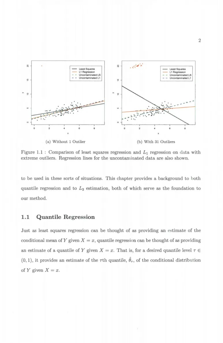
The differences in the effect that an outlier can have on these two forms of regres-sion are apparent in Figure 1.1(a), in which 99 points of bivariate normal data act as the uncontaminated data, in that there are no added outliers, and one extreme outlier is placed at (1, 20). As we can see, while there is little change in the L1 regression lines between using the full data set and the uncontaminated data, the least squares regression line is noticeably different.

However, situations can arise where L1 regression, and thus the prominent form of quantile regression, is affected by multiple outliers. In Figure 1.1(b), the same 99 points of uncontaminated data as before are plotted, but now with a cluster of 31 extreme outliers. Now, not only is the least squares regression line affected by the outliers, the L1 regression line is greatly affected as well. In situations as these, neither regression method provides a good summary of the uncontaminated data.

0 N

- Least Squares - L 1 Regression

Uncontaminated LS - - Uncontaminated L 1

(a) Without 1 Outlier

0 N

.

..

·.~~·,· \

.

- Least Squares - L 1 Regression Uncontaminated LS - - Uncontaminated L 1

.

._-:.

.

..

·~.-

..

··

·r.

:;

::.: ...

-,.

.

.

-

...

(b) With 31 Outliers

Figure 1.1 : Comparison of least squares regression and £1 regression on data with extreme outliers. Regression lines for the uncontaminated data are also shown.

to be used in these sorts of situations. This chapter provides a background to both

quantile regression and to £2 estimation, both of which serve as the foundation to our method.

1.1

Quantile Regression

Just as least squares regression can be thought of as providing an estimate of the conditional mean of Y given X= x, quantile regression can be thought of as providing

an estimate of a quantile of Y given X

=

x. That is, for a desired quantile level T E (0, 1), it provides an estimate of the Tth quantile,

Bn

of the conditional distribution

1.1.1 Koenker and Bassett's Approach

Although there are several methods, perhaps the most well known method of estimat-ing conditional quantiles is the method of quantile regression introduced by Koenker and Basset (1978). The idea stems from the £1 loss criterion, that is, absolute loss. It is well known that for a sample (x1 , x2 , . . . , xn) from a population X, the solution to the minimization problem

n

arg min

L

!xi - Ol

() i=l

is

0

=

x.50 , that is, the optimal value of

e

is the median of the sample. It is also known that we can use this criterion function to perform median regression. So, for example, if we wanted to find the coefficients f3 in a simple linear model that estimate the conditional median of Y on X, we would minimize the criterion

n

argmin

L

!Yi- Xi/31.

f3 i=l

Koenker and Bassett, hereafter referred to as KB, showed that by taking an asymmetrically-weighted absolute loss criterion, rather than the previous symmet-ric absolute loss criterion, other sample quantiles optimize the resulting minimization problem. Due to its appearance, an example of which is illustrated in Figure 1.3(b), Koenker calls this criterion function the "check" function. To see this, we define the check function for r E

(0,

1) by

{ -(1-r)x

Pr(x)

= TX if

X<

0 (1.1) if X~ 0.

Then, for a sample (x1 , x2 , ... , xn) from X, we solve the minimization

n

argmin LPr(Xi-0),

0 _i=l

(1.2)

which is equivalent to:

arg:nin

[I:

-(1- 7) *(xi-0)

+

L 7. (xi-

e)].

x;<O x;?_O

(1.3)

In order to find the optimal value of 0, we look at the first derivative with respect to

0 and find its root. Define no to be the number of observations in the sample that have a value less than 0:

2::(1-7)*(-1)+ 2::7=0

x;<O x;?.O

-no* (1- 7)

+ (n- no)* 7 =

0 -no+n*7 = 0.

Thus, the optimal value of

e

is the value such that no

= 7 *

n, that is, the value of

e

that lies above 7 * n values of the sample. In other words,

0

= x.,., the 7th quantile.

Just as the £1 loss criterion extends to median regression, the weighted absolute loss criterion extends to quantile regression. For a regression function g0(x) with parameter vector 0, if we minimize the residual error using a particular p.,. criterion function, that is,

n

argmin LPr(Yi- go(xi)), 0 _i=l

linear regression in two dimensions with a sample ((x1, y1 ), (x2, Y2), ... , (xn, Yn)) from (X, Y), if we use a linear regression function g(x) = a+x{3, our minimization becomes

n

arg min

L

Pr (Yi - a - xif3).

a,{3 i=l

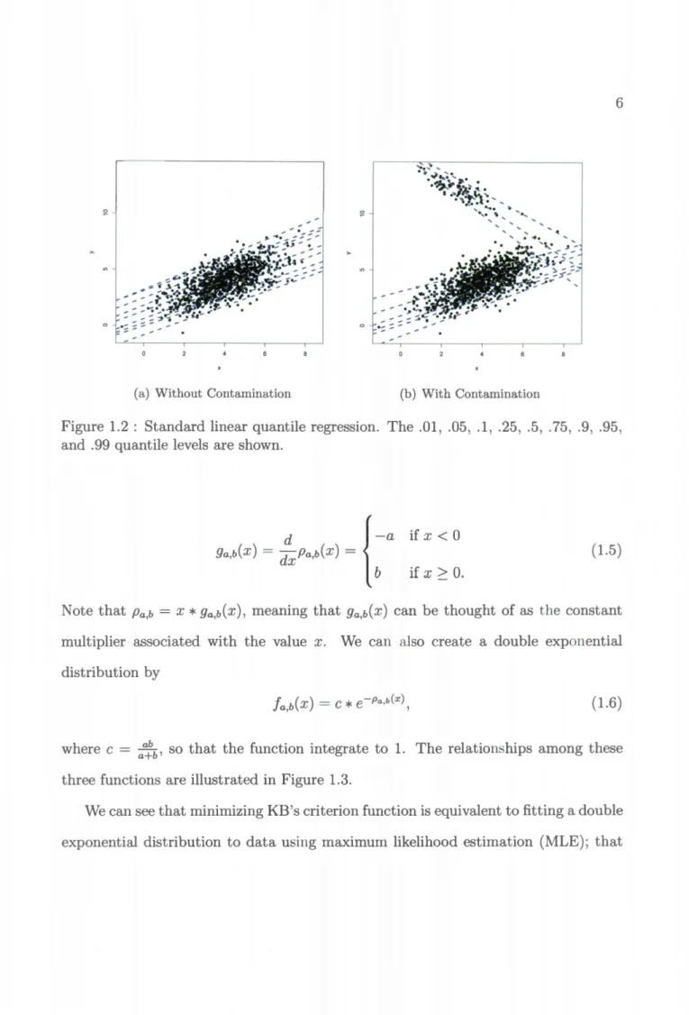
In Figure 1.2(a), examples of this simple linear quantile regression can be seen on 900 points multivariate normal data. In particular, the estimated .01, .05, .1, .25, .5, .75, .9, .95, and .99 quantile regression lines are shown.

Although quantile regression, like L1 regression, is considered more robust than least-squares regression, in that it is less affected by outliers, large numbers of outliers can cause large changes in the quantile estimation. In Figure 1.2(b), a cluster of 100 outlier points are added to the previous multivariate data as contamination. As we can see, when performing quantile regression for values ofT ~ .90, the regression line is now not only not passing through the original data, it is trending in the opposite direction of the original data.

1.1.2 Relationship to Maximum Likelihood

If we take a, b > 0, we can reparameterize the KB criterion function by

{ -ax Pa,b(x) = bx if

X<

0 (1.4) if X

2::

0.

It can be shown that this gives an equivalent minimization problem to the minimiza-tion in Equaminimiza-tion (1.2), where T = a!b· We introduce another function by

(a) Without Contamination (b) With Contamination

Figure 1.2: Standard linear quantile regression. The .01, .05, .1, .25, .5, .75, .9, .95,

and .99 quantile levels are shown.

d

{

-a

ga,b(x)

=

dxPa,b(x)

=

b

if X< 0

(1.5) if X~ 0.

Note that Pa,b

=

x

*

9a,b(x), meaning that 9a,b(x) can be thought of as the constant multiplier associated with the value x. We can also create a double exponential

distribution by

(1.6)

where c

=

a~b, so that the function integrate to 1. The relationships among the e three functions are illustrated in Figure 1.3.

We can see that minimizing KB's criterion function is equivalent to fitting a double

is,

b = 1 5

-a=-5

(a) 9a,b(x) (b) Pa,b(X) (c) !a,b(x)

Figure 1.3 : Relationship of functions with a= .5 and b

=

1.5.

arg ,:nin

t

Pa,b(x;-

0)

=

arg ;nax ( -

t

Pa,b(x; -

B))

= arg ~ax ( e-L:r=l Pa,b(xi-e))

n

=

arg max

IJ

!a,b(xi -B).

0 _i=l

b = 1 5

As with the choice of L1 error, this form of quantile regre sion does not have

an analytic solution for the MLE, as the derivative of Pa,b( x) is discontinuous, as

seen in Figure 1.3(a). Because of this, more complex methods are used to solve

this minimization problem. To solve the problem efficiently, Koenker (1987) uses a

modified version of the Simplex algorithm. In particular, he uses a modified version

of the algorithm presented by Barrodale and Robert (1973) for efficient L1 linear

approximation.

9a,b(x) function is created, making the derivative of the Pa,b(x) function analytic. Doing so allows us to use alternative optimization techniques, such as quasi-Newton algorithms, to solve the quantile problem. To create this smooth 9a,b(x), "S-curves", such as the cdf of a normal distribution or the cdf of a logistic distribution, are possible options. TheseS-curves are chosen due to their symmetry as well as their asymptotic nature as x ---+ ±oo.

In particular, we look at the cdf of a logistic distribution. We scale the function by (a

+

b), then shift the function both horizontally and vertically. This makes the asymptote as x---+ -oo = -a, the asymptote as x---+ oo

=

b, and makes the function pass through the origin. The general form of this S-curve is

a+b

g - a

a,b,c- 1

+

{-(a+b)*C*X

+

l (b)}- '

exp ab og

a

(1.7)

where c is a new tuning parameter that defines the slope of 9a,b,c as it passes through the origin. Thus, the greater the value of c, the steeper the slope at the origin.

From this new 9a,b,c function, we can build smooth versions of both the Pa,b and !a,b functions by

Pa,b,c(x)

=X*

9a,b,c(x) (1.8)

and

J,

_{a, ,c} b (x)

=

k

*

e-Pa,b,c(x) _' (1.9) where k is the normalizing constant that makes f~oo !a,b,c(x)dx = 1. The relationships of these new functions can be seen in Figure 1.4. For comparison, the KB versions of these functions are displayed in red. In Figure 1.5, the resulting functions are plotted for c

=

(.1, .5, 1, 2, 10). We can see that as c---+ oo, 9a,b,c ---+ 9a,b· Thus, Pa,b,c ---+ Pa,b

= 1 5

-a= 5

(a) 9a,b,c(x) (b) Pa,b,c(x) (c) fa,b,c(x)

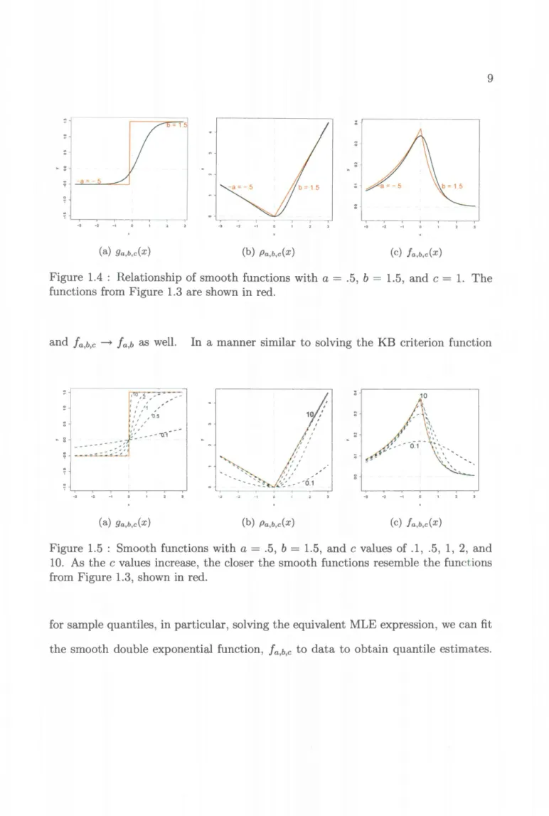
Figure 1.4 : Relationship of smooth functions with a

=

.5, b

=

1.5, and c

=

1. The

functions from Figure 1.3 are shown in red.

and !a,b,c - t !a,b as well. In a manner similar to solving the KB criterion function

t10 I~ 1, ,~ ' , , I I / _.,""' I I '1 / I 1 I ' t I ''0.5 I I 1 I I I I I I ! : - - - -l)~1 ... :; ---:~7 -~~

(a) 9a,b,c(x) (b) Pa,b,c(x) (c) fa,b,c(x)

Figure 1.5 : Smooth functions with a= .5, b

=

1.5, and c values of .1, .5, 1, 2, and

10. As the c values increase, the closer the smooth functions resemble the functions from Figure 1.3, shown in red.

for sample quantiles, in particular, solving the equivalent MLE expression, we can fit

That is, we can solve the maximization

n

{J = arg max

II

!a,b,c(Xi - e).

e i=l

(1.10)

However, which quantiles are estimated are no longer determined solely by the a and b

parameters in the double exponential. Instead, not only do those parameters matter,

the parameter c affects the estimate as well as the type of data itself, making this

method parametric. These effects can be seen in Figure 1.6. As we can see, when c

is large, the value of {J goes to the sample quantile, the same value the KB criterion

function estimates. However, when c is smaller, it tends to bring the estimate closer

to the median of the data.

(") ci N 0 0 0 0 -2 -1 Sample Quantile - - Double Exponentia - - f(x) [c =1] . . • f(x) [c = 10] 0 2 3

Figure 1.6 : MLE fits of standard double exponential and smooth double exponentials

on N(O, 1) data using a

=

.5 and b

=

1.5. The .75 sample quantile, as well as the

MLE fit of the standard double exponential distribution, is 0.699. The MLE fit of the smooth double exponential with c

=

1 is 0.566 while the fit with c

=

10 is 0. 700.

With this added complexity and parametric assumptions comes one advantage: theoretic quantiles estimated can now be determined using common analytic methods. In particular, this can be done maximizing the expectation. For example, if the data come from a N(O, 1) distribution, we can find the theoretic quantile achieved,

et,

as follows:

et

=

argmaxE[log(fa,b,c(X-

e))]= argminj

00

Pa,b,c(X-

e)*

¢(x)dx,

() () -oo

(1.11)

where ¢(x) is the pdf of a N(0,1) distribution. By using known values of a, b, and c and an assumed distribution for the data, we can derive theoretic quantile levels that the maximum likelihood will estimate. In Figure 1. 7, contour maps of these estimated quantile values can be seen for N(O, 1) data with a c = 1.

Estimation using maximum likelihood with the smooth double exponential also does not add any robustness to the estimation. Just as a large number of outliers will affect the estimation using the KB criterion function, using the smooth version will be similarly affected. To increase robustness, we must turn to a different method.

1.2

Density Estimation with

L

2

E

L2 estimation, or L2E, was developed by Scott (2001) as a robust, parametric density estimator. It belongs to a family of estimators, introduced by Basu et al (1998), but with special computational attractions. To estimate a density g(x) from a sample

(x1,

X2, ... ,

Xn)

by a family of distributions

j(x;

e),

we find the value of

e

by minimiz-ing a data-based estimator of integrated squared error. To see this, we consider

-2 -1 0 2

Figure 1.7: Theoretic MLE quantiles for N(O, 1) data with c

=

1

which expands to

arg:"in

J

f(x; B?dx- 2

J

f(x; B)g(x)dx +

J

g(x?dx. (1.13)

Because g(x) doesn't depend one, this minimization is equivalent to

arg:"in

J

f(x; B)2dx- 2

J

f(x; B)g(x)dx. (1.14)

The first term can be computed explicitly, as f(x; B) is a known distribution, while the

Thus, our L2E criterion can be estimated in a fully data-based fashion by

J

2 n

argmin f(x; 0) 2dx--

L

f(xi; 0).

o n i=l

(1.15)

For example, if we believe data to be from a normal distribution, ¢(xi; J-L, CT), we estimate the mean and variance parameters of the normal density, based on a sample (x1, x2, ... , Xn), by minimizing the quantity

(1.16)

which, after analyzing the integral, becomes

(1.17)

To illustrate this, we take a sample X =

(xi.

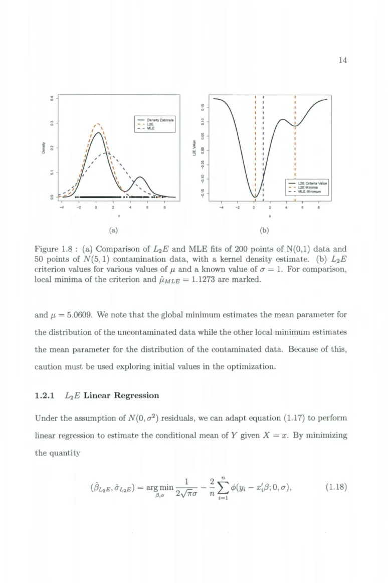
x2, ... , x250 ) with 200 points from a N(O, 1) distribution, which we consider our uncontaminated data, and 50 points from a N(5, 1) distribution, which we consider contamination. By minimizing the quantity in equation (1.17), we obtain estimates of ftL2E

= 0.1626 and

fJL2E

= 1.3380. However,

if we use maximum likelihood to estimate the parameters, we obtain ftMLE

= 1.1274

and fJMLE

= 2.2266. This is compared to the sample mean and standard deviation of

the uncontaminated data, ftsamp

= 0.1452 and

&samp

=

1.0663. A comparison of the

estimated density functions, along with a kernel density estimate of the data, can be seen in Figure 1.8(a).

Unlike MLE, the L2E equation is not convex. This is apparent in Figure 1.8(b), which shows a plot of the resulting values of the L2E equation for a range of J-L values and a known O"

= 1. Two distinct local minima can be seen, in particular at J-L

= 0.1528

~ "' 0 M 0 - Density Estimate - - L2E 0 0 - - MLE "' 0 0 i?:' ·~ _~ 0 0 0 0 0 ? 0 0 ? "' 0 0 0 -4 -2 -4 -2 (a) (b)

Figure 1.8 : (a) Comparison of L2E and MLE fits of 200 points of N(0,1) data and 50 points of N(5, 1) contamination data, with a kernel density estimate. (b) L2E criterion values for various values of 1-L and a known value of(]' = 1. For comparison,

local minima of the criterion and flMLE = 1.1273 are marked.

and 1-L = 5.0609. We note that the global minimum estimates the mean parameter for the distribution of the uncontaminated data while the other local minimum estimates the mean parameter for the distribution of the contaminated data. Because of this,

caution must be used exploring initial values in the optimization.

1.2.1 L2E Linear Regression

Under the assumption of N(O, (]'2

) residuals, we can adapt equation (1.17) to perform

linear regression to estimate the conditional mean of Y given X = x. By minimizing the quantity

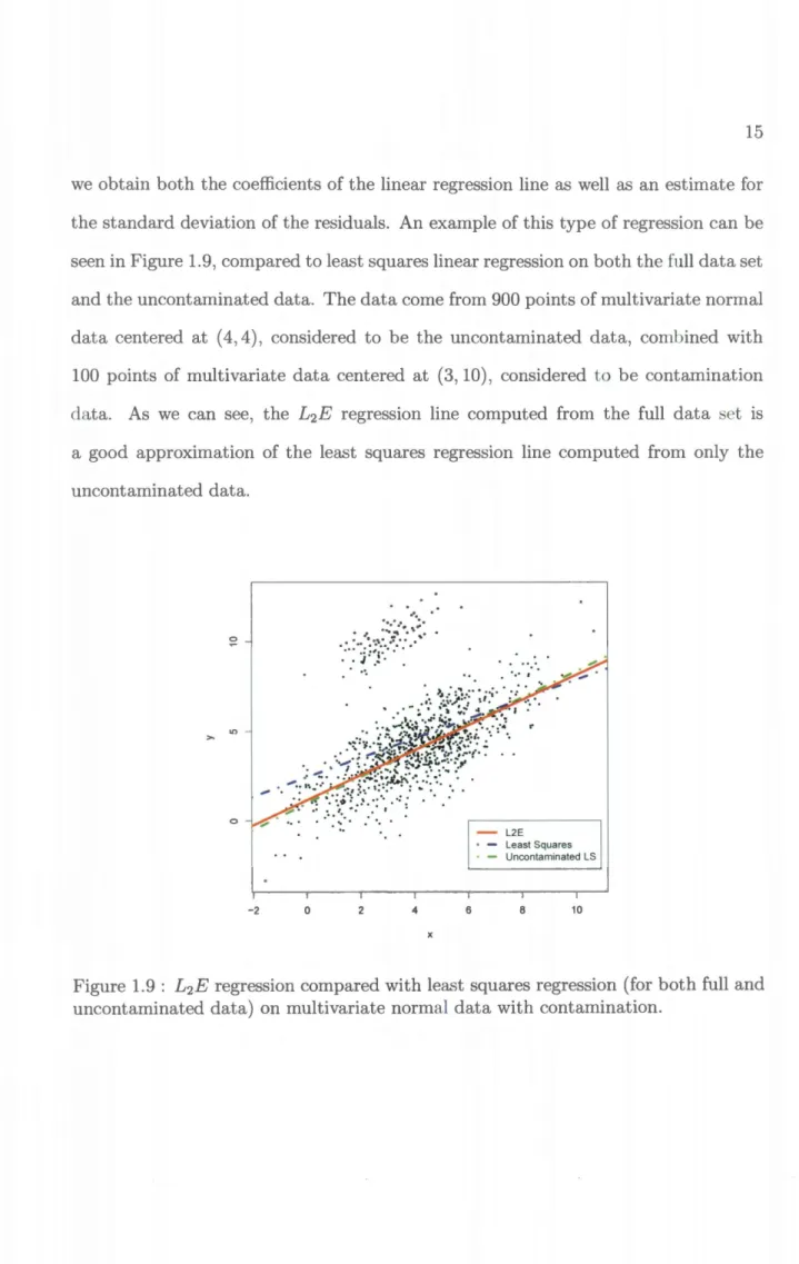
we obtain both the coefficients of the linear regression line as well as an estimate for the standard deviation of the residuals. An example of this type of regression can be

een in Figure 1.9, compared to least squares linear regression on both the full data set

and the uncontaminated data. The data come from 900 points of multivariate normal

data centered at ( 4, 4), considered to be the uncontaminated data, combined with

100 points of multivariate data centered at (3, 10), considered to be contamination

data. As we can see, the L2E regression line computed from the full data set is

a good approximation of the least squares regression line computed from only the uncontaminated data. 0 - L2E • - Least Squares • - Uncontaminated LS -2 0 2 4 6 8 10

Figure 1.9 : L2E regression compared with least squares regression (for both full and

1.3 Discussion

There are some situations where KB's quantile regression, that is, the generalization of £1 regression, can suffer issues with robustness. Therefore, in order to improve upon the robustness of quantile regression, £2E methods were examined for robust mean

regression to determine a similar way to adapt KB 's quantile regression. Chapter 2 describes the resulting £2E method that adds robustness to conditional quantile

estimation. The theory and asymptotic behavior of this method are discussed in Chapter 3. Nonlinear and semi-parametric applications are described in Chapter 4. Examples on simulated data with many outliers are shown in Chapter 5 while examples on real data are shown in Chapter 6.

Chapter 2

Robust Quantile Regression

As we have shown, L2E is able to be used as a robust density estimator and as a robust criteria for regression. From this, it is natural for us to believe that we can somehow use L2E as a robust quantile estimator and, from that, a robust criteria for quantile regression. From this, we can develop methods for both estimating the coefficients of a robust quantile regression model as well as the variances of those coefficients and a criteria to measure the fit of that model.

2.1 Estimating Quantiles with

L

2

E

Just as fitting a double exponential distribution to data using maximum likelihood obtains sample quantiles, we can obtain sample quantiles in a similar manner using L2E. In Equation (1.15), if we take f(x; 0) to be the double exponential function, that is { _QQ_ea(x-O) if X

<

0 f(x; 0)

=

fa,b(x - 0)

=

a+b a~be-b(x-0) if X ~ (}, (2.1)

we can minimize the quantity to estimate quantiles from a random sample from a known density function. The values of a and b affect the quantile estimated, as does the true distribution, g(x), making this method parametric. Our L2E minimization

estimate becomes

arg min

J

!a,b(x - 0)2_{dx -}

3_

t

_{!a,b(Xi - 0).}

8 n i=l

(2.2)

Given a distribution g(x), we can determine theoretic quantiles estimated by using L2E with a double exponential function given values of a and b. Using our known distributions g(x) and f(x; 0), we can evaluate the minimization in equation (1.14). In fact, because f(x; 0)

=

f(x- 0), the value of the first term in the equation doesn't depend on 0, reducing the minimization to

arg:nin -2

J

J(x; O)g(x)dx. (2.3)

Unlike the MLE, where the theoretic quantile level is known to be a:b' the values of a and b that achieve desired quantile levels vary depending on the distribution g(x). As seen in Section 3.1, it is possible for the theoretic quantile level to be a:b' such as in the case where g(x) "' Unif(O, 1), but that does not hold for all distributions. For example, if we wanted the .75 quantile when g(x) "' N(O, 1), and we apply the constraint a+ b = 2, we would use the values a= 0.382 and b = 1.618.

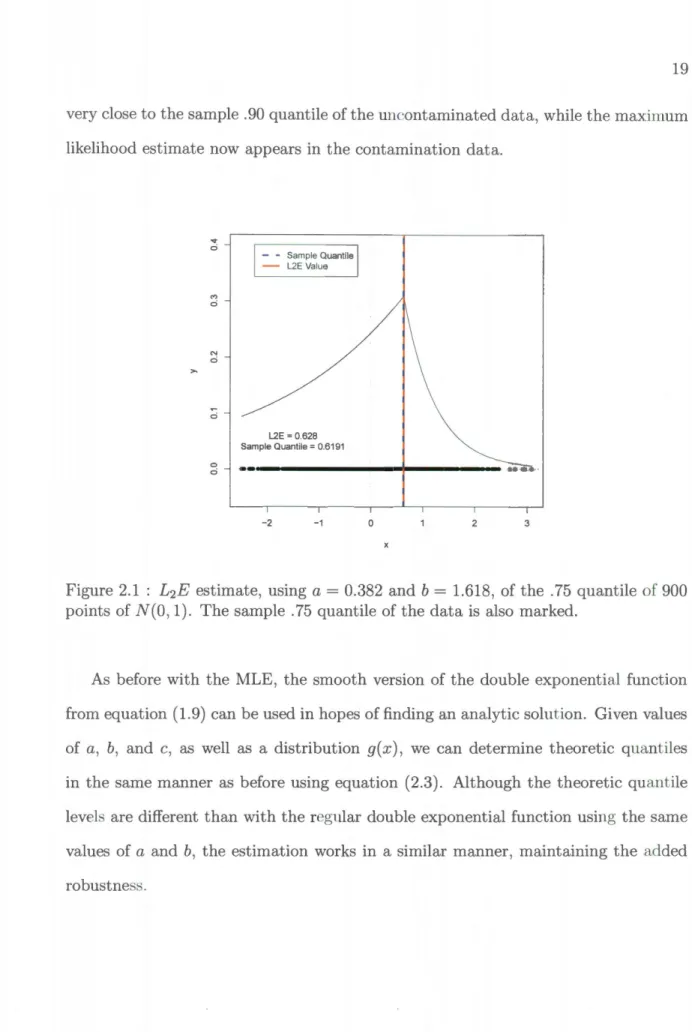
In Figure 2.1, a double exponential distribution with a= 0.382 and b = 1.618 are used to obtain the L2E estimate of the .75 quantile from 900 points of N(O, 1) data. As we can see, the estimated value of 0.6381 is very close to the sample quantile, 0.6101. In Figure 2.2(a), we can see that if we add 100 points of N(5, .1) contamination data to our sample, we still obtain a close estimate of the . 75 quantile of the uncontaminated data. In the plot, the red dot marks the . 75 quantile for the full data set, which is the maximum likelihood estimate. The added robustness of £2E is particularly apparent

very close to the sample .90 quantile of the uncontaminated data, while the maximum

likelihood estimate now appears in the contamination data.

N ci 0 ci - - Sample Quantile - L2E Value L2E = 0.628 Sample Quantile= 0.6191 -2 -1 0 2 3

Figure 2.1 : L2E estimate, using a

=

0.382 and b

=

1.618, of the . 75 quantile of 900

points of N(O, 1). The sample .75 quantile of the data is also marked.

As before with the MLE, the smooth version of the double exponential function

from equation (1.9) can be used in hopes of finding an analytic solution. Given values

of a, b, and c, as well as a distribution g( x), we can determine theoretic quantiles

in the same manner as before using equation (2.3). Although the theoretic quantile

levels are different than with the regular double exponential function using the same

values of a and b, the estimation works in a similar manner, maintaining the added

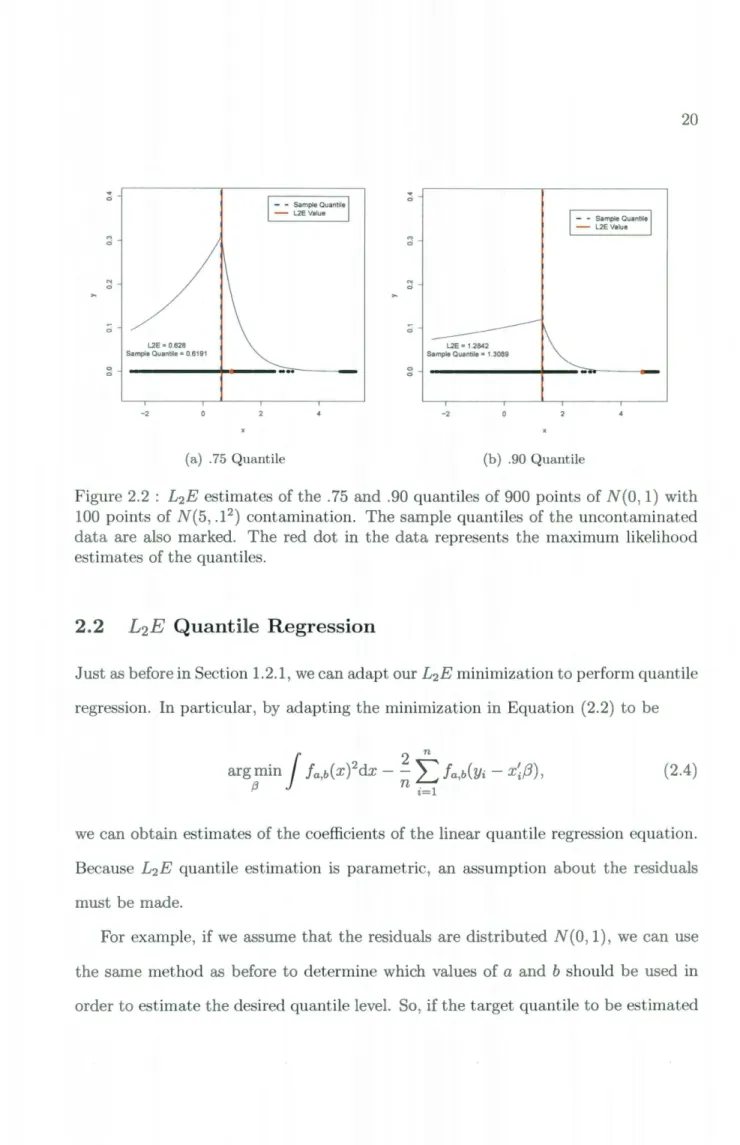
... 0 N ci ;; 0 0 L2E = 0.628 Sample Quantile = 0.6191 -2 (a) .75 Quantile ... ci M ci N ci ;; 0 0 -2 (b) . 90 Quantile

Figure 2.2 : L2E estimates of the .75 and .90 quantiles of 900 points of N(O, 1) with

100 points of N(5, .12

) contamination. The sample quantiles of the uncontaminated

data are also marked. The red dot in the data represents the maximum likelihood

estimates of the quantiles.

2.2

L

2

E

Quantile Regression

Just as before in Section 1.2.1, we can adapt our L2E minimization to perform quantile

regressiOn. In particular, by adapting the minimization in Equation (2.2) to be

(2.4)

we can obtain estimates of the coefficients of the linear quantile regression equation.

Because L2E quantile estimation is parametric, an assumption about the residuals

must be made.

For example, if we assume that the residuals are distributed N(O, 1), we can use

the same method as before to determine which values of a and b should be used in

was the . 75 quantile, setting a coefficient estimates.

0.382 and b - 1.618 would give us the desired

Figure 2.3 shows a comparison of L2E quantile regression with KB's quantile regression. The data set includes 900 points of bivariate normal data, generated such that the residuals around the mean line are approximated distributed N(O, 1), and 100 points of contamination data placed above the cloud of normal data. As we can see, the regression lines are similar for both the .01 quantile level and the .50 quantile level. However, once the desired quantile level goes above .90, the regression line from KB's method jumps up to the contamination cloud. As we can see in Figure 2.3(c), not only does the KB line pass through the contamination cloud, it trends the opposite direction from the uncontaminated data. However, the L2E regression line remains in the uncontaminated cloud, still providing an estimate of the .99 quantile of the non-contamination data. In Figure 2.4, we see a comparison of L2E quantile regression with KB's quantile regression on the full data set, as well as Koenker's quantile regression on the non-contaminated data.

Although we might be able to assume N(O, 0'2 ) residuals about the mean residual

line, assuming N(O, 1) is a stretch. However, if we are able to estimate 0' in a robust fashion first, we can still perform quantile regression. One such way to estimate 0' is to perform the L2E linear regression outlined in Section 1.2.1. This gives us a robust estimate of 0' which can then be used to either determine values of a and b by solving the minimization problem in Equation 2.3 to obtain the desired quantile, or to scale the data so that the residuals are distributed N(O, 1). To perform the latter option, we first obtain our estimate D-L2E, scale the data by dividing our response variable by

D-L2E, perform L2E quantile regression as we did before with our N(O, 1) residuals,

§

0.01

§

0.5 . ·.

. .

...

~·:

..

~ : .

.

;:::::/~f\·~~~u:!,.

(a) .01 quantile regression (b) .50 quantile regression

0.99

.. '· :• ·.. '

;

:·"i

{f

f~-~t~~~?

:.!'

.

(c) .99 quantile regression

Figure 2.3 : Comparison of L2E quantile regression, shown in red, and KB's quantile

regression, shown in blue, on 900 points of bivariate normal data with 100 points of

contamination added above. Least squares residuals are assumed to be N(O, 1)

Once again, we can replace the double exponential function, !a,b( x), in Equation

2.2 with the smooth double exponential function !a,b,c(x) to achieve similar results.

0 2 4 6 8

Figure 2.4 : Comparison of L2E quantile regression, shown in red, KB's quantile

regression on the full data set, shown in blue, and KB's quantile regression on the

uncontaminated data on 900 points of bivariate normal data with 100 points of

con-tamination added above. Least squares residuals are assumed to be N(O, 1)

can be seen in Figure 2.5, where the x-axis represents the desired quantile level and the y-axis represents the estimated value of the intercept and slope coefficients from L2E quantile regression for those desired quantile levels. These plots allow us to see

the different effects that each predictor variable across different quantile levels. As we can see, the coefficient estimates from using !a,b( x), shown in red, are noticeably less stable, as they bounce around the estimates from using !a,b,c(x), shown in black.

Because of this property, the smooth double exponential distribution will be used for

0 0

.

r

:

I

~

"' 0 0 0 "' "' 0

..

o:i 0 <0 0 "' 0 f?l 0 - Double Exponential - Smooth Double Exponential

"'

...

0

0.0 02 04 0.6 0.8 1 0 00 02 04 0.6 0.8 1 0

Quantile Quantile

(a) Intercept (b) Slope

Figure 2.5 : Comparison of the estimated slope and intercept coefficients for L2E

quantile regression using the same data found in Figure 2.4. L2E coefficient

esti-mates using the double exponential function, !a,b(x), are shown in red, while the _L2E

coefficient estimates using the smooth double exponential function, !a,b,c(x) are shown

in black.

2.2.1 Estimating Regression Coefficient Variances

As shown in Section 3.2.3, as n ---+ oo,

where

/3L

2

E

is the vector containing the quantile regression coefficients, {3* is the vector

of true coefficients, f~,b,c(s)

=

%sfa,b,c(s), and f~,b,c(s)

=

g

8 2

2!a,b,c(s). From this can estimate the covariance matrix of

[3

L₂E to be

l. _n ""'n (f' ( . - x'{J) )2

L...i=1 a,b,c Yz i [M' M]-1

where M is the n x

(p+

1) data matrix. We can use this estimated covariance matrix to estimate the variance of each coefficient. This allows us to create confidence intervals and p-values for each coefficient.

2.2.2 Model Selection Using AIC

As our solution to the minimization found in Equation 2.4 occurs when

i=l

we can treat our L2E quantile regression criteria as an M-estimator. Thus, we can ere-ate a robust Akaike Information Criterion (AIC) using the results found in Ronchetti (1997). That is, we can define the AIC for a L2E quantile regression model by

where

(J

is the vector of estimated L2E quantile regression coefficients and ap

=

2 tr(S-1

Q).

_Because

S

= -E[Hf3fa,b,c(Yi-

x~,B)]

= -E [f:,b,c(Y-

X',B)(XX')]

and

ap

reduces to

Q

= E[(\l{Jfa,b,c(Yi-

x~,B))] = E [

(f~,b,c(Y-

X',B)X)

(f~,b,c(Y-

X',B)X)']

=

E [ (

(f~,b,c(Y-

X',B))

2

(XX'))]

=

E [

(f~,b,c(Y-

X',B))

2_{] E [(XX')],} E [

(f~,b,c(Y

-

X'

,B))

2]

' -1

'

ap

=

-2

E[[J:,b,c(Y

_X' ,B)]

tr(E [(XX)] E

[(XX)])

E [

(f~,b,c(

E)) 2]

=

-2 E[[f"

(t:)) tr(Ip+l) a,b,c E [

(f~,b,c(

E)) 2]

=

-2 E[[f"

(t:))

(p

+

1),

a,b,c

where E has the assumed distribution of the residuals. This criterion acts in the same way as the standard AIC, in that models with lower AIC values are considered to be better fits to the data. Like Koenker (2005), in practice we use the median regression criterion to determine the model with the best fit for all quantile lines, although it may be possible to use this criterion with other quantile regression levels. We also note that in the implementation of our algorithm, the residuals are scaled for the model fit, so care must be taken as the scaling does have an effect on our criterion.

We believe that other information criteria developed for M-estimators, such as the Schwarz Information Criteria (SIC) described in Machado (1993), can be used to create additional model selection criteria for L2E quantile regression. For example,

the SIC can be shown to be

t,

(!

fa,b,c(x)2_{dx- 2fa,b,c(Yi-}

x~{3))

+

~(p

+

_l)log(n),

where p is the number of factors in the model. In initial testing, this SIC behaves very well on simulated data. However, it does not appear to behave as well as the AIC on real data. We postpone a detailed evaluation and comparison of AIC and SIC.

2.3 Discussion

In order to develop a robust method of estimating conditional quantiles, we turn to L2E density estimation and adapt it to estimate quantiles by taking ideas from KB's quantile estimation method. In doing so, we created a robust criteria, and an algorithm to use that criteria, that can be used to perform L2E quantile regression, giving us robust coefficients for linear models. Then, using methods developed for M-estimators, we are able to find estimates for variances of the regression coefficients as well as a robust version of AIC to assess model selection. The implementation of these ideas have been written in R, the function descriptions of which can be found in Appendix A.

Chapter 3

Theoretic Results

Having discussed how it is possible to perform robust quantile estimation using L2E, it is important to know how to select parameters for our estimator to achieve specific quantiles and how the selection of those parameters affect the accuracy of the esti-mator. To do so, in this chapter we examine both the theoretic results of our L2E quantile estimator as well as its asymptotic behavior.

3.1 Theoretic Values

When using L2E quantile estimation, it is of particular interest to know what values of a and b in our double exponential achieve specific quantiles. We recall that when we perform quantile estimation using KB's check function criteria, values of a and b achieve the a!b th quantile, regardless of distribution. L2E quantile regression,

however, requires a knowledge of the underlying distribution to determine which quantile is achieved by the values of

a

and b. That is, given a sample

(x

1 , x2, ... ,

xn)

from a population X with cdf G(x) and pdf g(x), can find the value

fh

2E that solves

the minimization

Note that because the first term does not depend one, as

e

is a shift parameter, it is a constant with regards to

e.

This allows us to reduce the minimization to

eL2E

= arg:nin -2

J

!a,b,c(x; O)g(x)dx. (3.1)

After finding eL2E in Equation 3.1, the theoretic quantile level estimated can be found by

If we want to determine values of a and b to achieve a particular quantile level, T, for a set value of c, we first determine the true quantile of X, denoted by

e

0 , by taking

e

0

=

c-

1(7). There are infinitely many combinations of a and b that can achieve this theoretic quantile, so we impose the restriction a + b

= r,

where r is a specified constant. From this, we find the value for a such that eL2E from Equation

3.1 is equal to

e

0 • Then, b can then be found as b = r- a.

For the following examples, we substitute the standard double exponential distri-bution, !a,b(x), for the smooth double exponential function, !a,b,c(x), in Equation 3.1. This was done to make the derivations in the examples simpler. However, the same methods apply when the smooth double exponential is used.

3.1.1 Uniform(O,l) Example

For given values of a and b and using a Uniform(O,l) distribution for g(x), we get from Equation 3.1

To solve this maximization, we take the derivative of the right hand side with respect to

e,

set the resulting equation equal to 0, and then solve for

e.

Thus, we get

-ae = -b+ be

ae

+be= b

From this, we see that an infinite number of combinations of a and b will achieve the same theoretic quantile value. Thus, to find a unique solution, it is necessary to restrict the values by setting a+b

=

r. Note that this is equivalent to the result found by the method presented by KB, particularly with a+ b

= 1. However, as evidenced

by the following section, this nice result does not hold for all possible distributions for g(x).

3.1.2 Standard Normal Example

Again for given values of a and band using a Normal(0,1) distribution for g(x), we get from Equation 3.1

[ J

1 _.,2 ]

BL2E

= arg:nin

-2 fa,b(x; B) v'2ife_2_dx

= argmax

[1()

kea(x-O) __ e-2-dx + 1 _.,2

1

1 ke-b(x-O) __ e-2-dx 1 _.,2 ]

() 0

v'2ii

()

v'2ii

= arg max

[ ke-a0+2 0.21() - - e 2 1

~

dx + keb0+2 b2100 - - e 2 1

~

dx ]

() - 0 0

v'2ii

() v'2ii

[

~ ~

]

= arg~ax

ke-aO+T4?(B- a)+ keb0+2 (1- 4?(B +b))

where 4?(x) is the cdf of a Normal(0,1) distribution. Taking the derivative with respect to

e,

setting the result equal to 0, and solving for

e,

we get

b2

- keb0+2 q;(e +b)

( ) b2 0.2

0

= -a4?(B- a)+ <P(B- a)+ be a+b 0+--y-

(1- 4?(e +b))

- e(a+b)O+b2;a.2 <P(B +b)

e(a+b)O+b2;a.2 = -a4?(e- a)+ <P(B- a) -b (1-4?(e +b))+ q;(e +b)

1 [ ¢(B-a)-a4?(B-a)] a-b

From this point, numerical approximation is necessary to solve for OL2E. Figure 3.1(a)

show the theoretic quantiles achieved by various combinations of a and b, presented in log10 scale. As shown in Figure 3.1(b), by selecting a value of r such that a+b = r, we can find a unique combination of a and b such that the resulting theoretic quantile eL2E gives <I>(OL2E)

=

T, where T is the desired quantile level. For the case shown, T = 0. 75 and r = 2. This gives the values of a = 0.382 and b = 1.618. This is different from the result given by KB, as these values of a and b would estimate a quantile level ofT= .809. As noted earlier, the L2E r's are closer to the median than the KB r's.

3.1.3 Robust Evaluation Via a Mixture of Uniforms

In order to see the effects of a mixture distribution on our L2E quantile estimation, we examine the simple case of a uniform mixture. Assume that without loss of generality we allow g(x) to be a mixture of a Uniform(0,1) distribution,with weight w E (0, 1) and a Uniform(u1,u2) distribution, with 1 < u1

< u2 and with weight (1-

w). Then for given values of a and b, we get from Equation 3.1

eL2E

= argmin [-2w

J

!a,b(x; 0)(1)dx- 2(1-w)

J

!a,b(x; e) 1 dx] . (3.2)

0 ~-~

Because of the nature of the double exponential distribution, we have to look at several cases. First, we examine the case that

e

E (0, 1), that is, a critical point within the range of the Unif(0,1) distribution. This gives us

-2w

t

kea(x-O)dx- 2w

11

ke-b(x-O)dx- 2(1-w)

1u2

ke-b(x-8)dx.

.0

i

I N I "' I N I "' I

~1

ol I -3 -2 -1 (a) Contours

~1

ol -j --3 -2 -1 log,o(a) ~0.001 -/'t A 0 A I · ~0001

-x

A 0 A

(b) Contours with a

+

b = 2 trace

Figure 3.1 : Contours of theoretic L2E quantiles for g(x) rv N(O, 1) for various values

of a and b, presented in log10 scale. Plot (b) includes a trace of a+ b

=

2 and marks

From this, we can see that the critical point in this region, if it exists, can be found by

From looking at the second derivative, we can see that this point is a local minimum of Equation 3.2. Next, we examine the case that f) E (1, u1 ), that is, a critical point between the ranges of the two uniform distributions. This gives us

The critical point in this region, if it exists, can be found by

From the second derivative, we see that this point is a local maximum of Equation 3.2. In the case where f) E (u~, u2 ), that is, a critical point within the range of the Unif(u1,u2 ) distribution, we get

The critical point in this region, if it exists, can be found by

ln [ eau1 -

w(~~~u

1

)

[ea-

lJ]

+

bu2

Again, from the second derivative, we find that this point is a local minimum of Equation 3.2. For the other two regions, namely 0

<

0 and 0

>

u2 , we can see that no critical points, and thus no local extrema exist. From all of this, we see that it is possible for our L2E equation to have two local minima.

For example, in the case where we have the mixture

~Unif(O,

1) +

~Unif(3,

4),

there are two local minima, as exhibited in Figure 3.2(a). However, if have the case where we have the mixture

~Unif(O,

1) +

~Unif(2,

3),

there is only a single local minimum, as seen in Figure 3.2(b).

3.2

Asymptotic Theory

In order to determine the asymptotic behavior of of estimate, OL2E, we begin once again with the minimization

I

2 n

arg min !a,b(x - 0)2dx - -

L

!a,b(Xi - 0).

e n i=I

(3.3)

This has a minimum when the derivative with respect to 0 is equal to 0. Again, because the first term does not depend on 0, this is equivalent to finding 0 such that

1 n

a

- L

aofa,b(Xi-0)

= 0.

n i=I

N c::i I '<t c::i I <0 c::i I 00 c::i I 0 I N c::i I '<t c::i I <0 c::i I 00 c::i I 0 I "'! I -1 -1 0 3 4 5

(a) ~Unif(O, 1)

+

%Unif(3, 4)

0 2 4

(b) tUnif(O, 1)

+

tUnif(2,3)

Figure 3.2 : L2E criteria values for values of

e

with g(x) being a mixture of two

This allows us to treat our L2E estimate as an M-Estimator and use the same meth-ods, such as those described in Van der Vatt (2000), to show asymptotic normality. To do this, we define

'1/Jo(xi)

=

%ofa,b(xi-

e) and Wn(e)

=

~ 'L:~=l

'fo(xi)·

From here, we perform the Taylor expansion of Wn(e) about the desired quantile value, that is,

eo and find that

Where e is some value between eL2E and e. Examining the right hand side, we first see that -v'n'llln(eo)

= -

Jnwn(eo), which by the Central Limit Theorem has a Normal distribution with mean = 0 and a variance that can be found by

We also see that

and that

The same result holds if the smooth double exponential distribution, !a,b,c(x) is used in place of the standard double exponential distribution, !a,b(x).

3.2.1 Uniform(O,l) Example

We take g(x) to be the Uniform(O,l) distribution and values of a and b such that the theoretic value of fh2E

= 0

0 , where 00

=

a!b

=

T. From this, we see that

J (:

0Ja,b (x- 0))2 g(x)dx =

1°

[a2k 2e2a(x-O)] dx

+

1

1

[b2k2e-2b(x-O)] dx

=

~k2

[a- ae-2aO] -

~k2

[be-2b(1-0)- b]

2 2

1

=

2k2 [a+ b- ae-2aO- be-2b(1-0)]

and also

:(} J

:(}fa,b(x- O)g(x)dx

= :(}

[1°

[-akea(x-O)]dx +

1

1 [bke-b(x-O)]dx]

=

~

[ke-ao- k- ke-b( 1-0)

+

k]

8(}

= -kae-ao - kbe-b(1-0).

Therefore, we have

The theoretic standard deviations for a range of values of a and b can be found in Figure 3.3(a).

3.2.2 Standard Normal Example

If we instead take g(x) to be the standard Normal(O,l) distribution and values of a and b such that the theoretic value of

fh

2E = 00 , where <1>(00 ) = T. We then see that

and also

aja

ao

aofa,b(X-

O)g(x)dx

=

~

[10 [ -akea(x-O)J _1_e

-;2 dx +

1oo [bke-b(x-O)J _1_e

-;2 dx]

aO

-oo

..j'i;

0

..j'i;

a [

k -aO+a210 1 -(x-a)2 d bk bO+b21oo 1 -(x+b)2 d ]

= -

-a e - - e 2 x

+

e - - e 2 x

aO

-oo

..j'i;

0

..j'i;

=

:o [

-ake-a0+a2<I>(O- a)+ bkebO+b2

[1-

<1>(0

+

b)J]

=

a2_{ke-a0+a2<I>(O-a)- ake-aO+a2 ¢(0- a)}

The theoretic standard deviations for a range of values of a and b can be found in Figure 3.3(b).

3.2.3 L2E Linear Quantile Regression Coefficients

One area of particular interest is the asymptotic behavior of the coefficient estimates of our L2E quantile regression. We know that given the linear model

y

= X'{J +

t:,

the criterion function for L2E linear quantile regression is

where !a,b,c is the smooth version of the double exponential distribution, Yi are iid from random variable Y, {3 = {{30 , {31 , ... , {Jp} and Xi = {1, xil, ... , Xip}, which are iid from random variable X, we see that the solution to this minimization occurs when

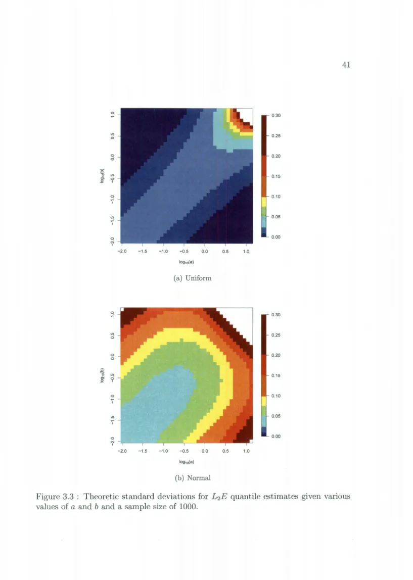
~ Oi .Q .c Oi .Q 0 l() c::i 0 c::i l() c::i I 0 I ~ I 0 N I 0 l() c::i 0 c::i l() c::i _I Cl I ~ I 0 N I -2.0 -1.5 -1.0 -2.0 -1.5 -1.0 0.30 0.25 0.20 0.15 0.10 0.05 0.00 -0.5 0.0 0.5 1.0 log10(a) (a) Uniform 0.30 0.25 0.20 0.15 0.10 0.05 0.00 -0.5 0.0 0.5 1.0 (b) Normal

Figure 3.3 : Theoretic standard deviations for L2E quantile estimates given various values of a and b and a sample size of 1000.

Let /3* be the value such that

E[v

1da,b,c(Y- X'/3*)]

=

Op+I·

Then, by performing a Taylor expansion around {3., we see that

Op+l

=

.!_

t

\7(3Ja,b,c(Yi-

x~/3*)

+

.!_

t

Hf3fa,b,c(Yi-

x~f3)(f3L

2

E-

/3.)

n i=I n i=I

1 n 1 n

-2::::

Hf3fa,b,c(Yi-

x~f3)(f3L

2

E-

/3.)

= --

2::::

\7(3Ja,b,c(Yi-

X~/3.)

n i=I n i=l

(/3L,E - /3.)

~

[

~

t,

Hpfo,o,,(Y; -

x;/3)

]-l [-

~

t,

'\1 p/o,b,o(Yt -

X:/3.)]

Vn(/3 L,e- /3.)

~

[

~

t,

H pfo,o,,(Y; -

X:/3)

r [-

Jn

t,

'\1 P f o,o,o(y; -

x:/3.)

l·

It can be shown that

where

f~,b,c(s)

= :

₈Ja,b,c(s),

and

where

where Also, E

= E[('V!1fa,b,c(Y- X'{3*))(\7!1fa,b,c(Y- X'{3*))']

= E [ (-

f~,b,c(Y-

X'{J*)X) (-

J~,b,c(Y-

X'{J*)X)']

= E [

(f~,b,c(Y-

X'{3*))2 _(XX')]

= E [

(f~,b,c(t))

2

]

E [(XX')].

~

tH!1fa,b,c(Yi-

x~{3)-+

E[H!1fa,b,c(Y- X'f3)] i=l

= E [f:,b,c(Y- X'{J*)(XX')]

= E [f:,b,c(t)] E[(XX')] =V.

where the covariance matrix reduces to

v-

1

_EV-

1

=

_(E

[f:,b,c(t:)] E[(XX')])-1

_{E [}

(f~,b,c(t:))

2

]

_{E [(XX')]} X

(E

[f:,b,c(t:)] E[(XX')])-1

E

[(f~bc(t:))

2

]

= ,; ' 2

E[(XX')t1E[(XX')]E[(XX')t1

E

[fa,b,c(t:)]

=

E

[U~,b,c(~:))2]

E[(XX')]-1.

E

[f:,b,c(t:)]2

From this, given distributions for both X and the error, ~:, we can determine the asymptotic covariance matrix of our regression coefficients. We can also estimate this result using our data to come up with an estimate of the covariance matrix of our regression coefficients, such as in Section 2.2.1.

3.3 Simulated Results

3.3.1 Quantile Estimates for Mixtures

To examine the effect of contamination on our L2E quantile estimates, we examine three separate mixture densities. For each mixture, a range of weights, w, and pa-rameters were examined in which 1000 points of data were simulated 1000 times, with 1000w points coming from the true density and 1000(1- w) points coming from the contamination density. A double exponential distribution with a = b = 1 was used for the L2E criteria, estimating the median of each distribution. The average minimum over the simulations for each combination was then used to make the contour plots in Figure 3.4. In each contour plot, the areas where there are two theoretic minima are shaded blue, while the areas where there is a single theoretic minimum are shaded

red.

The first mixture, shown in Figure 3.4(a), is a mixture of a Unif(0,1) distribution, considered the true density, and a Unif(d, d + 1) distribution, where d

>

1 is the left endpoint of the contamination density. That is, the mixture density can be represented by

wUnif(O, 1) + (1- w)Unif(d, d + 1).

The region to the right of the 0.51 contour line are combinations of the weight and the contamination left endpoint that have simulated means of 0.50

± 0.01. We can

see that as w and d increase, the bias added to the estimated values of 8L2E by the contamination density decreases. In particular, once there is a large enough difference between the two distributions in the mixture, the estimate within the uncontaminated density is not very affected by the contamination density, regardless of the weight.

The second mixture, shown in Figure 3.4(b), is a mixture of a Unif(0,1) distri-bution, again considered the true density, and a Unif(1,s + 1) distridistri-bution, where s

>

0 is the width of the contamination density. Thus, the mixture density can be represented by

wUnif(O, 1) + (1- w)Unif(1, 1 + s).

Though not as drastic as the previous mixture, we see that increasing the parameters wands decreases the bias on the estimated values of 8L2E. We can also see from this mixture is that if there is no separation between the two densities in the mixture, we will see an effect on the estimate within the uncontaminated region, adding bias towards the contamination.

The third mixture, shown in Figure 3.4(c), is a mixture of a N(0,1) distribution, considered the true density, and a N(J.L,1) distribution, considered the contamination

density. This mixture can be represented by

wN(O, 1) + (1- w)N(fL, 1).

The region to the right of the 0.01 contour line are combinations of the weight and the contamination mean that have simulated means of 0

±

0.01. Once again, by increasing w and fL, the bias caused by the contamination density on the estimated values of eL2E decreases. As before in the first mixture, when there is a large enough separation between the two densities, the estimate within the uncontaminated density is not very affected by the contamination density, regardless of the weight.

3.3.2 Standard Deviation

To verify the theoretic standard deviations found in Section 3.2, a range of combina-tions of a and b we simulate 10,000 samples of Uniform(0,1) data of size 1000. We keep track of the estimated values of OL2E for each sample. The standard deviations of

these estimated values of OL2E for each pair of a and b can be found in Figure 3.5(a).

We repeat this process using Normal(0,1) data of size 1000, the results of which can be found in Figure 3.5(b). As we can see, these simulated results closely match both the theoretic values and the trends of those values found in Figure 3.3. This lends credence to our formulas for asymptotic behavior of OL2E. One trend of note that is featured in both plots is the monotonicity of the standard deviation across the median, that is, when a = b, as a+ b, increases. This leads us to believe that smaller values of r cause our estimate to have a smaller standard deviation. However, this is not the only consideration to be taken into account when selecting a value of r.

"' ~ "' 0 CX) 0 1'-0 CD 0 "' 0 10 Left Endpoint (a) wUnif(O, 1) + (1- w)Unif(LE, LE + 1) 0 ...: "' 0 CX) 0 .c "' ~ 1'-0 CD 0 "' 0 .c "' ~ Mean 0 ...: "' 0 CX) 0 1'-0 CD 0 "' 0 10 Wdth

(b) wUnif(O, 1) + (1- w)Unif(1, 1 +Width)

10

(c) wN(O, 1) + (1- w)N(J-L, 1)

Figure 3.4 : Theoretic quantiles estimated from various mixture models. The red

regions indicate L2E criteria with one theoretic minimum while blue regions indicate

.0 o; .2 ~ o; .2 0 lO c:i 0 c:i lO c:i I 0 I lO I 0 N I Cl lO c:i 0 c:i lO c:i I 0 I ~ I 0 N _I -2.0 -1.5 -2.0 -1.5 0.30 0.25 0.20 0.15 0.10 0.05 0.00 -1.0 -0.5 00 0.5 1.0 (a) Uniform 0.30 0.25 0.20 0.15 0.10 0.05 0.00 -1.0 -0.5 0.0 0.5 1.0 (b) Normal

Figure 3.5 : Simulated standard deviations for L2E quantile estimates given various

3.4 Choosing a Value of r

As mentioned in Section 3.1, to find unique solutions to our L2E minimization in Equation 3.1, it is necessary to set a+ b equal to some constant r. Ideally, this value of r minimizes the variance for all values of T, giving us as accurate of an estimator as possible. For our purposes, we will examine the case where g(x) = N(O, 1). As shown by the curves in Figure 3.6, variance goes down as r goes to 0. This property is illustrated in Figure 3. 7, where the standard deviations at each quantile for traces of r = .01, 1, 2, and 10 are shown.

However, we still need a value of r that gives us good numeric results when we are using our L2E quantile estimator. In Figure 3.8, we again see the theoretic quantile contours for N(O, 1) data. Curves representing a+ b =rare plotted on the contours, where r = .01, 1, 2, and 10. As we can see, if we have too small of a value of r, it can be difficult for extreme quantiles to be estimated, as either the value of a or b has to be so small that it can affect the optimization. Because we want the smallest value of r possible that can estimate the extreme quantiles without having a or b be too close to 0, we propose that an r somewhere around 2 is a reasonable choice.

3.5

Discussion

As we can see, given the parameters a and b for our L2E quantile estimation criteria and an assumed distribution g(x) for the data, we are able to determine which theo-retic quantile values are being estimated. Likewise, we are able to choose a and b to achieve a specific quantile level, T, such that the theoretic quantile estimate

fh

2E, is

equal to

c-

1(7). We can also determine the asymptotic behavior of our estimate, al-lowing us to determine its distribution. The asymptotic behavior, along with the step

e

0 0> _Q L() c) 0 c) L() c) I ~ ...-I ~ ...-I ~ N I -2.0 -1.5 -1.0 -0.5 0.0 0.5 1.0

Figure 3.6 : Standard deviations for each quantile curve. At each point on the curve, the width of the curve is proportional to the standard deviation of 8 L2E for those

values of a and b. From the bottom, the .01, .05, .1, .25, .5, .75, .9, .95, and .99 quantile levels are shown.