Semiparametric Multivariate Density Estimation Using Copulas and Shape-Constraints

(1)

SEMIPARAMETRIC MULTIVARIATE DENSITY ESTIMATION USING COPULAS AND SHAPE-CONSTRAINTS

SAWITREE BOONPATCHARANON

A DISSERTATION SUBMITTED TO THE FACULTY OF GRADUATE STUDIES

IN PARTIAL FULFILMENT OF THE REQUIREMENTS FOR THE DEGREE OF

DOCTOR OF PHILOSOPHY

GRADUATE PROGRAM IN MATHEMATICS AND STATISTICS YORK UNIVERSITY

TORONTO, ONTARIO

May 2019

(2)

Abstract

Maximum likelihood estimation of a log-concave density has certain advantages over other nonparametric approaches, such as kernel density estimation, which re-quires a bandwidth selection. Furthermore, finding the optimal bandwidth gets more

difficult as a dimension increases. On the other hand, the shape-constrained approach is automatic and does not need any tuning parameters. However, for both the kernel and log-concave estimators, the rate of convergence slows down as the dimension d increases. To handle this “curse of dimensionality”, we study an intermediate semi-parametric copula approach and we estimate the marginals using the log-concave shape-constrained MLE and use a parametric approach to fit the copula parameters.

We prove √n rate of convergence for the parametric estimator and that the joint density converges at a rate of n−2/5 _{regardless of dimension. This is faster than the}

conjectured rate ofn−2/(d+4) _{for the multivariate log-concave estimators [Cule, 2009].}

We examine the performance of our proposed method via simulation studies and real data example.

(3)

Acknowledgements

This thesis would not be submitted without support from a number of people. I would like to thanks my supervisor Dr. Hanna Jankowski for her numerous helpful and valuable guidance since I am a Ph.D. student at York University. I also would

like to thanks my committee members, Dr. H´el`ene Massam and Dr. Xin Gao, for

their comments both in dissertation subject oral exam and colloquium dissertations. Those comments are significant for improving this thesis. I also want to thanks all

the staff members and friends for their helpful in several ways. Moreover, I would like to thanks my family for thier supports and always stand by my side. Finally, I would like to special thanks to my sponsorship, Chulalongkorn University, Thailand

(4)

List of Tables

1.1 Convergence rate for density estimators . . . 17

4.1 Copulas in the simulation study . . . 71

4.2 Details of specification cases . . . 74

4.3 Details of misspecification cases . . . 75

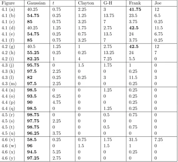
4.4 % of how often each copula has been selected with BIC . . . 78

6.1 Details for the simulation study . . . 130

6.2 Classification results of case I: average number of misclassification cases from 100 simulation sets where the number in brackets are per-centages from (6.7) . . . 131

6.3 Classification results of case II: average number of misclassification cases from 100 simulation sets where the number in brackets are per-centages from (6.7) . . . 132

(10)

9.1 Details for simulation study . . . 156 9.2 Clustering results for univariate case . . . 157

(11)

List of Figures

1.1 Kernel density estimation of standard Gaussian with several

band-width selections in the same graph of using log-concave density esti-mation and true density . . . 14

2.1 Estimated density from log-concave MLE with a true density of

stan-dard Gaussian distribution . . . 26 2.2 Logarithm density of standard Gaussian distribution with the vertical

dotted lines represent the locations of knots . . . 28 2.3 Tent-like structure for the logarithm of MLE when d=2 (Figure from

Cule et al. [2010]) . . . 35

(12)

4.1 MISE for d=2 MLE, parametric IFM, log-concave IFM, kernel IFM, kernel IFM with G-L, multivariate log-concave, and

multivariate kernel . . . 79 4.2 MISE for d=2 MLE, parametric IFM, log-concave IFM,

kernel IFM, kernel IFM with G-L, multivariate log-concave, and

multivariate kernel . . . 80 4.3 MISE for d=4 MLE, parametric IFM, log-concave IFM,

kernel IFM, multivariate log-concave, and multivariate kernel. . . . 81 4.4 MISE for d=5 MLE, parametric IFM, log-concave IFM,

kernel IFM, and multivariate kernel. . . 82 4.5 MISE for d=6 MLE, parametric IFM, log-concave IFM,

kernel IFM, and multivariate kernel. . . 83 4.6 MISE from top left to bottom right: d=2,d=4,d=5, andd=6 MLE,

parametric IFM, log-concave IFM, kernel IFM, multivariate

log-concave, and multivariate kernel. . . 84 4.7 MISE for two-parameter copula when d = 2 MLE, parametric

IFM, log-concave IFM, kernel IFM, and multivariate kernel. . . 85

5.1 Study √n rate of convergence forN(0,1) . . . 115 5.2 Study √n rate of convergence for Γ(2,1) . . . 116

(13)

5.3 Study √n rate of convergence fort5 . . . 117

5.4 Estimated rate of convergence for ˆθwhen f0(x) =eα0xh0(x) . . . 118

7.1 Breast cancer data with benign as light grey dots and malignant as

dark grey dots . . . 135 7.2 Surface plots for Breast cancer data set from (a) Gaussian mixture model (b)

mixture of Frank copula with log-concave marginals (c) multivariate log-concave

mixture . . . 136 7.3 Contour plots with misclassification cases (benign as light grey dots and malignant

as dark grey dots) for Breast cancer data set from (a) Gaussian mixture model (b)

mixture of Frank copula with log-concave marginals (c) multivariate log-concave

mixture . . . 136 7.4 Contour plots with misclassification cases for Breast cancer data set from (a)

Gaussian mixture model (b) mixture of Frank copula with log-concave marginals

(c) multivariate log-concave mixture; each symbol is for misclassification cases in● all methods,◾both GMM & multivariate log-concave mixture,▴GMM & copula model, ◆ copula model & multivariate log-concave mixture, × only multivariate log-concave mixture,+only copula model,◯only GMM . . . 137

8.1 D-vine with 6 dimensions, 5 trees and 15 edges . . . 143 8.2 C-vine with 6 dimensions, 5 trees and 15 edges . . . 144

(14)

1

Introduction

1.1

Motivation

Multivariate density estimation is a common and much studied problem in

statis-tics. When we have d-dimensional independent and identically distributed (i.i.d.) data, say X1, X2, . . . , Xn ∈Rd, the ideal way to estimate a density f is using para-metric density estimation in which the true distribution function needs to be known.

However, in several cases, we do not have any clue for the distribution of f. The general way to estimate f is to use nonparametric approaches, which require fewer assumptions than parametric approaches and do not need information about the

distributions.

When we have no idea about the distribution of data, we can easily consider the distribution function as a step function, which jumps up by 1/n at each point of observation. We call this idea an empirical cumulative distribution function. How-ever, it is not a density function, so it is not our preferred approach. The popular

(15)

nonparametric density estimation is a kernel density estimation, which requires a good bandwidth selection in order to have a good density estimation. However, a

bandwidth parameter is not easy to find, but we can choose this smoothing param-eter by using a cross-validation approach or normal reference rule, (see Wasserman [2006] for more details). However, the bandwidth selection will be an issue when the

dimension,d, is getting large because, instead of choosing one bandwidth parameter for one-dimensional data, you need to define a bandwidth matrix with its dimension according to the data’s dimension. For example, when your data have four

dimen-sions, your bandwidth will be a 4×4 matrix, which has a symmetric and positive definite property. Furthermore, there is a tradeoff between bias and variance, be-cause, if you choose too large a bandwidth, the bias will be huge while the variance

small. This event is an oversmoothing problem. On the contrary, if your bandwidth is too small, you will get an undersmoothing density estimation. Further details of kernel density can be found in Section 1.2.2.3.

To overcome the difficulty of bandwidth selection, a shape-restricted density es-timation has been introduced and has become more popular in recent years. Instead of dealing with the additional tuning parameters, the shape-constrained density

esti-mation works with some good characteristics of its functions. Such examples include monotonic, unimodal, or log-concavity. Among several shape-constrained models,

(16)

our work focuses on the log-concave densities.

One advantage of the log-concave density estimation above the kernel density

es-timation is that it does not need any tuning parameters. Furthermore, a log-concave maximum likelihood estimator always exists and is unique, and it can be done auto-matically. However, the multivariate log-concave MLE is computationally intensive,

which makes the algorithm not friendly in practice. The univariate log-concave ML estimator converges with raten−2/5_{, but the conjectured rate of convergence for}

mul-tivariate log-concave ML estimator is n−2/(d+4)_{, which depends on the dimension} _d

(see Cule [2009]). This makes the estimators from multivariate log-concave distribu-tions have much slower convergence rate than the univariate log-concave, especially when d is large.

Sklar [1959] introduced a dependence modeling called “copula”. The copula is a function, which splits joint distribution function to its one-dimensional marginal distributions and dependence part with its parameters, which are called the copula

parameters. Suppose we observe n i.i.d. random variables X = (X1, . . . , Xn) ∈ Rd, let fj(xj) be the univariate marginal density functions of X in dimension jth with corresponding cumulative distribution functions Fj(s) = ∫

s

−∞fj(r)dr;j = 1, . . . , d.

(17)

be represented in this form f(x1, . . . , xd) =c(F1(x1), . . . , Fd(xd);θ) d ∏ j=1 fj(xj), (1.1)

wherefj can be any parametric or nonparametric univariate density functions. Sim-ilary,crepresents the dependence ofddimensions and its density can be chosen from several well-known copula families (more details in Chapter 3). Copula models have been widely used in recent years, for example, in finance, see Jouanin et al. [2011]

and epidemiology, see Chen [2012].

The main objective of this thesis is to improve the rate of convergence and com-putational time for multivariate log-concave density estimators by using the copula

model with univariate log-concave marginals. We propose the semiparametric den-sity estimation for _Rd_{, where the main tools of our study are the copula models} together with the univariate log-concave densities. We work on estimating the

den-sity in equation (1.1) by applying the method from Joe [2005], which has been widely used in recent years. This method has been called an “inference function for mar-gins” (IFM). It is a two-stage estimation method which estimates marginal densities

and copula parameters separately.

Moreover, we also prove that our proposed semiparametric density estimation method converges at a rate of n−2/5_{, and the rate of convergence for the copula}

(18)

estimators mentioned in Cule [2009], which is n−2/(d+4)_{. However, the convergence}

rate of the copula estimators is never better than a parametric ML estimators, which

converge at a rate of n−1/2_.

In this chapter, we will discuss each type of density estimation, which belong to the parametric density estimations in Section 1.2.1, to the nonparametric density

estimations in Section 1.2.2, and to the semiparametric density estimations in Section 1.2.4. The nonparametric density estimations that we will focus on consist of the empirical cumulative distribution function, the histogram, and the kernel density

estimation. The log-concave density estimation will be presented in Section 1.2.3. In addition, the rate of convergence for each method will be summarized in Section 1.3.

1.2

Density estimation

1.2.1 Parametric density estimation

LetX = {X1, X2, . . . , Xn} ∼F be theni.i.d. random variables from a distribution function, F, with a probability density, f =F′_{, the density estimation of} _f _{can be}

(19)

the density f with distribution’s parameter(s) θ∈Θ can be expressed as L(x∣θ) = n ∏ i=1 fθ(xi).

Then, we get a log-likelihood function

`(x∣θ) = n

∑

i=1

logfθ(xi). (1.2)

To simplify, we denote `(x∣θ) as `(θ). Then, we maximize (1.2) to get a maximum likelihood estimator ̂θn, which

̂

θn=argmax θ∈Θ

`(θ).

Hence, the density estimator of f can be expressed as f̂n(x) = f_θ̂

n(x). In several

distributions, θ̂n has a closed form, for instance, Gaussian, exponential, Poisson, binomial and also other distributions in exponential family. This makes parametric approach easy to use. Moreover, the parametric maximum likelihood estimator under the regularity conditions also satisfies a convergence rate ofn−1/2_{, which is the fastest}

rate among other density estimation methods.

1.2.2 Nonparametric density estimation

Knowing the distribution functions of data is hard in practice. Therefore, the parametric density estimation may not be a good choice. The nonparametric

(20)

ap-proaches were introduced because they can model the unknown distribution func-tions. For example, the upcoming method has the fewest assumptions for

estimat-ing distributions by just givestimat-ing a mass 1/n to each observation. For the

follow-ing nonparametric methods, suppose we observe n i.i.d. random variables, X =

{X1, X2, . . . , Xn}, from an unknown density f.

1.2.2.1 Empirical cumulative distribution function

Definition of the cumulative distribution function (CDF) isF(t) =P(X≤t). We can estimateF(t) by ̂ Fn(t) = 1 n n ∑ i=1 1xi≤t.

We callF̂n(t)an empirical CDF, which can be found by not assuming any underlying distributions to the data. However, the empirical CDF is a mass function, which is not a density function. It means that this method may not be a desired answer for

(21)

1.2.2.2 Histogram

One of the simple nonparametric density estimations is histogram, which is not a smooth function. The density estimator for n observations can be represented as

̂ fn(x) = m ∑ j=1 ̂ pj h1Bj(x),

where Bj are the jth bin. B1 = [0,_m1), B2 = [_m1,_m2), . . . , Bm = [m_m−1,1], where m is the total number of bins. The binwidth h equals 1/m. Let Aj be the number of observations inBj, then p̂j =Aj/n.

Theorem 1.1. (Wasserman [2006], Theorem 6.9) Consider fixed x and fixed m, let

Bj be the bin containing x and let pj= ∫_B_jf(u)du. Then, E( ̂fn(x)) = E(̂ pj) h = pj h = ∫Bjf(u)du h ≈ f(x)h h =f(x) and V ar( ̂fn(x)) = pj(1−pj) nh2 .

The expectation and variance in Theorem 1.1 are calculated with respect to the random quantity f̂n which depends onX1, . . . , Xn. When h approaches zero, f̂n(x) will become an unbiased estimator, however its variance will become large. It turns out that choosing a reasonable h is necessary for histogram.

A convergence rate of this estimator is computed via a risk function, which is

calculated from an expectation of an integrated square loss function. Let R and L denote a risk function and a loss function, respectively. The risk function is given by

(22)

R=E(L), where

L= ∫ ( ̂fn(x) −f(x))

2

dx.

Theorem 1.2. (Wasserman [2006], Theorem 6.11) Suppose that f′ _{is absolutely}

continuous and that _{∫ (}f′(_u))2_du< ∞_{. Then}

R( ̂fn, f) = h2 12∫ (f ′(_u))2_du+ 1 nh+o(h 2_{) +}_o₍1 n). (1.3)

A value h∗ _{that minimizes} _(1.3) _is

h∗= 1 n1/3 ( 6 ∫ (f′(_u))2_du) 1/3 .

With this choice of bandwidth,

R( ̂fn, f) ≈

(3/4)2/3(∫ (_f′(_u))2_du)1/3

n2/3 .

Hence, when we choose the optimal h∗_{, the risk decreases to zero at a rate of} n−2/3_. _{It means the histogram density estimator converges with a rate of} _n−1/3_,

which is slower than a rate ofn−1/2 _{from the parametric density estimation.}

1.2.2.3 Kernel density estimation

A kernel density estimation is another simple and well known nonparametric density estimation. A kernel is a smooth functionK such thatK(x) ≥0,_∫ K(x)dx=

(23)

1,_∫ xK(x)dx=0,andσ2

K = ∫ x2K(x)dx>0. There are several choices of kernel such as Gaussian kernel: K(x) = √1 2πe −x2/2_, boxcar kernel: K(x) = 1₂1[−1,1](x), Epanechnikov kernel: K(x) = 3 4(1−x2)1[−1,1](x).

One-dimensional density estimation of n observations with a bandwidth h and a kernelK can be written in this form

̂ fn(x) = 1 nh n ∑ i=1 K(x−xi h ).

An effect of the bandwidth selection can be clearly seen in Figure 1.1. Furthermore,

the risk function for a kernel estimator is presented in the following theorem.

Theorem 1.3. (Wasserman [2006], Theorem 6.28) Let R= ∫ E(f(x) − ̂f(x))2_dx _be

the integrated risk. Assume thatf′′_{is absolutely continuous and that}

∫ (f′′′(_x))2_dx< ∞. Then, R( ̂fn, f) = 1 4σ 4 Kh 4 n∫ (f ′′( x))2dx+ ∫ K 2(_x)_dx nh +O( 1 n) +O(h 6 n), (1.4) where σ2 K = ∫ x2K(x)dx. The optimal h ∗ _{that minimizes} _(1.4) _is h∗= ( ∫ K(x) 2_dx n(∫ x2_K(_x)_dx)2_{∫ (}_f′′(_x))2_dx) 1/5 .

Plug in h∗ _into _(1.4)_{, we get}

(24)

Therefore, the kernel density estimator converges with a rate of n−2/5_{, which is}

faster thann−1/3 _{from the histogram. However, it is still slower than} _n−1/2 _{from the}

parametric MLE.

For d > 1, suppose we have n i.i.d random variables Xi = (Xi1, . . . , Xid);i = 1, . . . , n, then the density estimator with a bandwidth matrix H is given by

̂ fn(x) = 1 n n ∑ i=1 KH(x−xi), (1.5)

whereH is ad×dsymmetric and positive definite matrix. K is a multivariate kernel function withKH(x) = ∣H∣−1/2K(H−1/2x). A popular kernel function is a multivariate Gaussian kernel, which can be written in this form

KH(x) = (2π)−d/2∣H∣−1/2exp{− 1 2x

T_H−1 x},

where H plays the role of a covariance matrix. From (1.5), to avoid building the bandwidth matrix H, we can estimate f at x = (x1, . . . , xd) by using the following formula ̂ fn(x) = 1 nh1⋯hd n ∑ i=1 {∏d j=1 K(xj −xij hj )},

whereh1, . . . , hd denote the bandwidth for each dimension.

For multivariate kernel estimator, the risk function can be expressed as

R( ̂fn, f) ≈ 1 σ_K4 ⎡⎢⎢⎢ d ∑h4_j_∫ f_jj2(x)dx+ ∑h2_jh2_k_∫ fjjfkkdx⎤⎥⎥⎥+(∫ K2(_x)_dx)d 1⋯ ,

(25)

wherefjj denote the second partial derivative of f. The optimal bandwidth satisfies hi=O(n−1/(d+4)). Therefore, the risk converges to zero at a rateO(n−4/(d+4)), which leads us to the density estimator with a rate of convergencen−2/(d+4)_.

To summarize, one-dimensional kernel density estimator converges with the rate n−2/5_{, which is slower than} _n−1/2 _{of the parametric ML estimator. On the other hand,}

the rate of convergence of multivariate kernel density estimator is n−2/(d+4)_{, which is}

the slowest density estimation method in our work.

1.2.3 Log-concave density estimation

Suppose we observe n independent random variables X = {X1, X2, . . . , Xn} from an unknown density f ∶ _R ↦ [0,∞) where f(x) is said to be a univariate log-concave density if f(x) = expϕ(x) for some concave functions ϕ ∶ _R ↦ [−∞,∞). The corresponding cumulative distribution function off isF(x) = ∫_−∞x f(r)dr.

A maximum likelihood estimation (MLE) of the log-concave density gets more attention in recent years, because its ML estimator always exists and is unique, (see

D¨umbgen and Rufibach [2009]). The MLE of log-concave densities has an obvious

advantage above the kernel density estimation, because it is fully automatic and it does not need any smoothing parameters. We can clearly see from Figure 1.1 that the

(26)

studies of log-concave distributions become more popular - see, for example, the work from Walther [2002]. This is the first paper that discussed the log-concave

distribu-tions in a statistical aspect. They worked on one kind of shape restricted maximum likelihood inference, called log-concavity. Walther [2009] showed a good explanation of log-concave distributions and an application in a clustering problem. Moreover,

the class of log-concave distributions contains various common parametric distribu-tions such as Gaussian, Γ(α, β) with α ≥ 1, β(a, b) with both parameters greater than 1, Weibull(α) with α ≥ 1, Laplace, and exponential distributions. Moreover,

D¨umbgen and Rufibach [2009] showed the uniform consistency of a nonparametric

ML estimator for one-dimensional log-concave densities. Balabdaoui et al. [2009, Theorem 2.1, page 1305] also showed that the log-concave density estimator f̂n and the piecewise linear ϕ̂n converge pointwise to the true density f and the true ϕ0

with the rate n−2/5 _{and characterized the limiting distributions. Furthermore, Doss}

and Wellner [2016, Theorem 3.2, page 9] proved that the univariate log-concave ML

estimator has a global rate of convergence at a raten−2/5_{under the Hellinger distance.}

For multidimensional log-concave distributions, Cule [2009] studied the limiting behavior of the log-concave ML estimator and conjectured that the rate of

conver-gence with respect to the Hellinger bracketing entropy isn−2/(d+4)_{for all}_d_{. This rate}

(27)

Figure 1.1: Kernel density estimation of standard Gaussian with several bandwidth selections in the same graph of using log-concave density estimation and true density

this rate depends on d, the multidimensional log-concave MLE is computationally intensive especially when d is high. Moreover, Cule et al. [2010] presented some attractive theoretical properties of the multivariate log-concave MLE both when the model is log-concave and when it is a misspecified model.

1.2.4 Semiparametric density estimation

In between parametric and nonparametric models, we have a semiparametric model, which is a statistical model in which some parameters do not belong to a

Euclidean space but lie in an infinite dimensional space. A log-concave space, which is a nonparametric space, is the infinite dimensional space that we work on. In order

(28)

to estimate the joint density function, we integrate the parametric copula model together with the univariate log-concave densities.

As we discussed in the previous section that finding the multivariate log-concave density estimator is computationally intensive which is because of the curse of dimen-sionality problem. To overcome this issue, we use the univariate log-concave density

estimation and the copula model as our proposed density estimation method. Hence, our proposed semiparametric model is given by

f(x1, . . . , xd;F1, . . . , Fd, θ) =c(F1(x1), . . . , Fd(xd);θ) d

∏

j=1

expϕj(xj).

Estimating this model will be done in two stages where the first stage is to find the log-concave ML estimators for each marginal density separately. Then, we estimate the copula parameter. This is a reason why the proposed method performs faster

than the multivariate log-concave MLE, since it is not depend on the dimension. Note that all marginals do not depend on the copula parameters. A log-likelihood function for estimating the copula parameters is given by

n

∑

i=1

logc( ̂F1(x1), . . . ,F̂d(xd);θ). (1.6)

̂

θ from maximizing (1.6) is also the θ that would solve

n−1

n

∑

i=1

(29)

Hence, estimating the copula parameter can be viewed as a Z-estimation, which Z denote the zero from setting the above score function equals to zero. Moreover, the

copula estimator from (1.7) can be called as a “Z-estimator”.

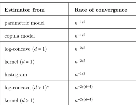
Furthermore, we prove that the Z-estimator is consistent and converges at rate n−1/2_{. Moreover, the joint density estimator converges at rate} _n−2/5 _{regardless of}

dimension. This rate makes our proposed semiparametric density estimator con-verges faster than the multivariate log-concave MLE and multivariate kernel density estimation. However, it is still slower than the parametric model.

1.3

Rate of convergence

Table 1.1 shows the rates of convergence for all density estimators that have been

(30)

Table 1.1: Convergence rate for density estimators

Estimator from Rate of convergence

parametric model n−1/2 copula model n−1/2 log-concave (d=1) n−2/5 kernel (d=1) n−2/5 histogram n−1/3 log-concave (d>1)∗ _n−2/(d+4) kernel (d>1) n−2/(d+4)

Note: * is a conjectured rate of convergence for alld.

1.4

Outline

The organization of this thesis is as follows. In Chapter 2, we discuss the log-concave density estimation both in the univariate and multivariate cases. The

avail-able R packages,logcondensandLogConcDEAD, that use to calculate the log-concave ML estimators will be mentioned with details of their algorithms. We also show the theoretical parts, which are pointwise limiting distributions and global rates

(31)

LogConcDEAD package to estimate the multivariate log-concave ML estimators are presented in the form of computational time.

In Chapter 3, we present the copula model to solve the curse of dimensionality

problem. This chapter will talk about several copula families such as Gaussian

copula and Archimedean copula families. Note that we only focus on parametric

copula families. The details of semiparametric Z-estimation will be summarized, and the two-stage estimation method will also be discussed. Moreover, some literature reviews about the asymptotic relative efficiency of the two-stage estimation method

and the MLE method will be presented in this chapter too.

Some simulation studies are shown in Chapter 4. The performance on the den-sity estimation of our proposed method and other parametric, nonparametric and

semiparametric methods will be presented.

The main theorems and proofs are in Chapter 5. We will show that the copula estimators under the log-concave marginals satisfy the consitency property and has

√

n convergence rate. Therefore, the joint density estimator by using the copula model with the log-concave marginals converges at a rate n−2/5_{, irrespective of the}

dimension. Some necessary regularity conditions and assumptions for proving the

main theorems also be demonstrated at the end of this chapter.

(32)

shown in Chapter 7 where the background of finite mixture models and expectation-maximization (EM) algorithm will be presented in Chapter 6. Some further

exten-sions will be discussed in Chapter 8. In this chapter, we focus on vine copulas, which allow us to account for the multiple dependence structures.

Other than the main part of this thesis, we work on another applied project.

This project works on the univariate log-concave densities. We do some simulation studies on clustering problems and proposed a new criterion for selecting the number of subpopulations. We call this criterion as a “proposed BIC”. This application is

(33)

2

Log-concave density estimation

2.1

Definitions and properties

A function f is said to be concave if

f(λx+ (1−λ)y) ≥ λf(x) + (1−λ)f(y)

for all x, y ∈ _Rd _and _λ ∈ (₀_,₁)_. _{We also say that a density} _f _{will be a log-concave} density if logf is concave. LetX1, X2, . . . , Xnbe independent random variables from some unknown densities f ∶ _R ↦ [0,∞), the log-concave density function can be expressed as

f(x) =expϕ(x). (2.1)

From (2.1), we also have logf(x) = ϕ(x), for some concave functions ϕ ∶ _R →

[−∞,∞). The cumulative distibution function (CDF) can be represented as F(x) =

(34)

Example 2.1. Gaussian distribution f(x) = 1 2πσ2exp{− 1 2σ2(x−µ) 2_}_; _µ_{∈ [−∞}_,_∞]_{, σ}2 _>₀ logf(x) = −log(2πσ2) − 1 2σ2(x−µ) 2 ∂xlogf(x) = − (x−µ) σ2 ∂_x2logf(x) = − 1

σ2 concave for all x

Example 2.2. Weibull distribution

f(x) = k λ( x λ) k−1 e−(x/λ)k ; x≥0, k, λ>0 logf(x) =logk λ+ (k−1)log x λ− ( x λ) k ∂xlogf(x) = k−1 x − k λ( x λ) k−1 ∂_x2logf(x) = −k−1 x2 − k(k−1) λ2 ( x λ) k−2

not concave when k<1 F(x) =1−e−(x/λ)k_; _x≥₀_{, k, λ}>₀ logF(x) = (x λ) k ∂xlogF(x) = k λ( x λ) k−1 ∂2 xlogF(x) = k(k−1) λ2 ( x λ) k−2 concave when k<1

(35)

Example 2.3. gamma distribution f(x) = β α Γ(α)x α−1 e−βx ; α, β>0

logf(x) =αlogβ−log Γ(α) + (α−1)logx−βx ∂xlogf(x) =

α−1 x −β ∂_x2logf(x) = 1−α

x2 concave for α≥1

Moreover, the log-concave shape constraint is attractive for various reasons. Some

of them are as follows.

1. Most common parametric distributions such as Gaussian, gamma with shape

parameter ≥ 1, beta with both parameters ≥ 1, exponential, Laplace, Weibull with shape parameter≥1 are log-concave. In contrast, some distributions are not log-concave for all values of parameters, for instance, Cauchy, log-normal,

F, and Student’s t-distribution.

2. The cumulative distribution function (CDF) of all log-concave functions are log-concave. Nevertheless, some non log-concave densities have log-concave

CDFs such as log-normal, gamma when shape parameter < 1, and Weibull

when shape parameter <1, (see Example 2.2).

3. All marginal and conditional of log-concave densities are again log-concave.

(36)

4. All log-concave densities are unimodal, but not all unimodals are log-concave. According to Birg´e [1997, Definition 1], a density f of the realines is called

unimodal if there exists some number M (not necessary unique) such that f

is nondecreasing on (−∞, M) and nonincreasing on (M,+∞). Any suchM is called a mode of the density. The densityf is said to be decreasing iff =0 for x<M and increasing if f =0 forx>M.

5. Log-concave is called a strongly unimodal density. (Ibragimov [1956]) A distri-bution function is called strong unimodal if its composition with any unimodal

distribution function is unimodal.

6. The sum of two independent log-concave random variables is log-concave whereas a unimodal class does not satisfy this attractive property.

7. The nonparametric ML estimator of the log-concave density always exists and

is unique. The corresponding theorem is shown in D¨umbgen and Rufibach

[2009, Theorem 2.1] and its proof is in D¨umbgen et al. [2011, Section 2]. On

the contrary, the nonparametric ML estimator of a unimodal density does not exist, see Birg´e [1997].

8. Balabdaoui et al. [2009] proved that the pointwise limiting distribution is

n2/5( ̂_f

(37)

Furthermore, Doss and Wellner [2016] showed that the univariate log-concave ML estimator has a global rate of convergence at a rate ofn−2/5_{. This rate was}

proved with respect to the Hellinger metric. On the other hand, the nonpara-metric ML estimator of the unimodal density converges at a slower rate than the log-concave ML estimator. The rate is n−1/3_.

9. The rate of convergence for univariate log-concave density estimator is better thann−2/(d+4)_{, which is the conjectured rate of multivariate log-concave density}

estimator and multivariate kernel density estimator.

10. The use of log-concave densities appears in several applications. Chang and Walther [2007] presented clustering with a mixture model. They extend an EM algorithm to work with the univariate log-concave densities and compare

the simulation results with the Gaussian mixture model (GMM). It shows that modeling with the log-concave densities has smaller misclassification cases than the GMM especially when the distributions are non-normal.

(38)

2.2

One-dimensional log-concave density

2.2.1 Log-concave maximum likelihood estimation

According to the density in (2.1), a log-likelihood function can be expressed as

`(ϕ) = 1 n n ∑ i=1 ϕ(xi).

Then, we add a Lagrange term to `(ϕ) in order to relax a constraint of f being a density. Moreover, the objective function in (2.2) will be set to maximize over all concave functions and will still satisfy the equation of_∫ expϕ̂(t)dt=1, see Silverman [1982]. Therefore, the modified log-likelihood function is given by

`mod(ϕ) = 1 n n ∑ i=1 ϕ(xi) − ∫ R expϕ(t)dt. (2.2)

Hence, the nonparametric ML estimator of ϕ is the maximizer of the function

(2.2) over all concave functions, which can be represented as

̂

ϕn=argmax ϕ concave

`mod(ϕ).

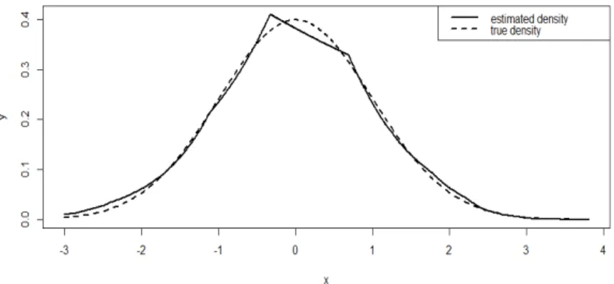
We also show a comparison between the estimated density from the log-concave ML

estimator and the true density in Figure 2.1. Moreover, D¨umbgen and Rufibach

[2009] showed that there exists a unique concave function ϕ̂n that maximizes the `mod(ϕ) function. In the next section, we will present some properties ofϕ̂n.

(39)

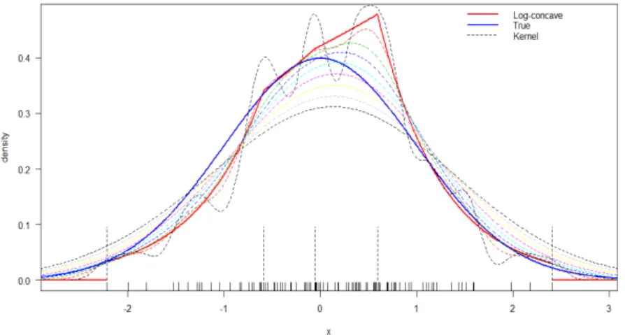
Figure 2.1: Estimated density from log-concave MLE with a true density of standard Gaussian distribution

2.2.2 Log-concave density estimator ϕ̂n

We denoteSnas a set of all knots from some continuous piecewise linear functions gn∶ [X(1), X(n)] ↦R, whereX(1)< ⋅ ⋅ ⋅ <X(n)denote an order statistics ofX1, . . . , Xn.

The set of knots can be represented as

Sn(gn) ∶= {u∈ (X(1), X(n)) ∶g ′

n(u−) >g

′

n(u+)} ∪ {X(1), X(n)}. (2.3)

As we can see, knots occur when the function changes slope. The minimum and maximum observations always are knots. The density estimation is of the form

̂

fn(x) =expϕ̂n(x). Figure 2.2 shows the estimated logarithm function of standard Gaussian distribution where its knots represent at the vertical dashed line.

(40)

More-over, f̂n = 0 outside the data range since ϕ̂n = −∞. The followings are some other characterizations of knots.

ϕ̂n occur at some points of data in [X(1), X(n)]. This is different from k

-monotone density fork>1 where the knots always lie between observations.

According to D¨umbgen and Rufibach [2009], for x≥X(1), let

̂ Fn(x) ∶= ∫ x X(1) expϕ̂n(u)du, ̂ Gn(x) ∶= ∫ x X(1) ̂ Fn(u)du, Gn(x) ∶= ∫ x X(1) Fn(u)du= ∫ x −∞F n(u)du.

Then, the concave functionϕ̂n is the ML estimator of the log-density ϕ0 if and

only if ̂ Gn(x) ⎧⎪⎪⎪ ⎪⎪⎪⎪ ⎨⎪⎪ ⎪⎪⎪⎪⎪ ⎩ ≤Gn(x) ∀x≥X(1), =Gn(x) if x∈ Sn(̂ϕn).

A consequence from the previous characterization of ϕ̂n is that the estimator of the distribution function F̂n is close to the empirical distribution function Fn onSn(̂ϕn).

(41)

Figure 2.2: Logarithm density of standard Gaussian distribution with the vertical dotted lines represent the locations of knots

2.2.3 A computational aspect of the univariate log-concave MLE

Theorem 2.4. [D¨umbgen and Rufibach, 2009] The nonparametric ML estimator

̂

ϕn exists and is unique. It is linear on all intervals [Xi, Xi+1], 1≤i<n. Moreover,

̂

ϕn= −∞ on R/[X(1), X(n)].

From Theorem 2.4, expϕ(t) from (2.2) can be written as a linear function for each interval of [Xi, Xi+1]. We define Si+1 as a slope of x∈ [Xi, Xi+1]. Hence,

Si+1 =

ϕi+1−ϕi xi+1−xi .

(42)

Then, the second term of`mod(ϕ)in (2.2) can be expressed as ∫ R expϕ(t) dt = n−1 ∑ i=1 ∫ xi+1 xi eϕi+(t−xi)Si+1 _dt = n∑−1 i=1 (eϕi+1 −eϕi) (xi+1−xi ϕi+1−ϕi ).

Now we can write (2.2) in an explicit form, which is

`∗(_ϕ) = 1 n n ∑ i=1 ϕ(xi) − n−1 ∑ i=1 (eϕi+1−eϕi) (xi+1−xi ϕi+1−ϕi ).

Finding one-dimensional log-concave ML estimator is quite convenient because

there is an available package in R called logcondens. This package is built by

D¨umbgen and Rufibach [2011] and can be accessible from CRAN at http://CRAN.

R-project.org/package=logcondens. According to their work, they presented two algorithms for calculating the univariate log-concave ML estimator, which are itera-tive convex minorant algorithm (ICMA) and acitera-tive set algorithm (ASA). According

to Walther [2009], ASA appears to be an efficient algorithm to calculate the MLE

nowadays. Thus, we decide to use ASA, which is implemented by D¨umbgen et al.

[2011], in our thesis. The ASA is a useful tool from optimization theory, see Fletcher

[1987]. The main idea of this algorithm is that it solves a finite number of uncon-strained optimization problems, see D¨umbgen et al. [2011, Section 3]. A function for finding the log-concave ML estimator in logcondens package with ASA is

(43)

activeSet-2.2.4 Auxiliary results for d=1

Gradient and Hessian matrices of f are also important to be studied. Since the expressions of these two matrices are complicated, we introduce a new auxiliary

function J, which can rewrite the partial derivatives of (2.2) in terms of the J

functions. The following J functions will be discussed again in Chapter 9 when

we calculate a criterion for choosing the number of subpopulations in the clustering

problem. We will show the expressions of these two matrices only for one-dimensional data. First, the modified log-likelihood function can be represented in the term ofJ function, which is given by

`∗( ϕ) = 1 n n ∑ i=1 ϕ(xi) − n−1 ∑ i=1 J(ϕi, ϕi+1)(xi+1−xi).

The J function can be expressed as

J(ϕj, ϕk) =J(ϕk, ϕj) = ⎧⎪⎪⎪ ⎪⎪⎪⎪ ⎨⎪⎪ ⎪⎪⎪⎪⎪ ⎩ exp(ϕk)−exp(ϕj) ϕk−ϕj if ϕj≠ϕk, exp(ϕj) if ϕj =ϕk, (2.4)

with the fact that J(ϕj, ϕk) = exp(ϕj)J(0, ϕk−ϕj). In addition, J(0,0) = 1 and J(0, r) = exp(r)−1

r . Letting Jpq(ϕj, ϕk) =∂ p ϕj∂

q

(44)

gradient and Hessian matrices of `∗(_ϕ)_{when we have} _m _{knots are given by} ∂ϕj` ∗( ϕ) = ⎧⎪⎪⎪ ⎪⎪⎪⎪⎪ ⎪⎪⎪⎪⎪ ⎨⎪⎪ ⎪⎪⎪⎪⎪ ⎪⎪⎪⎪⎪ ⎪⎩ 1 n−∆1J10(ϕ1, ϕ2) for j=1, 1 n−∆jJ10(ϕj, ϕj+1) −∆j−1J01(ϕj−1, ϕj) for 2≤j<m, 1 n−∆n−1J01(ϕm−1, ϕm) for j=m. (2.5) −∂ϕj∂ϕk` ∗( ϕ) = ⎧⎪⎪⎪ ⎪⎪⎪⎪⎪ ⎪⎪⎪⎪⎪ ⎪⎪⎪⎪⎪ ⎪⎪⎪⎪⎪ ⎪⎪ ⎨⎪⎪ ⎪⎪⎪⎪⎪ ⎪⎪⎪⎪⎪ ⎪⎪⎪⎪⎪ ⎪⎪⎪⎪⎪ ⎪⎪⎪⎩ ∆1J20(ϕ1, ϕ2) for j =k=1, ∆jJ20(ϕj, ϕj+1) −∆j−1J02(ϕj−1, ϕj) for 2≤j =k<m, ∆n−1J02(ϕn−1, ϕm) forj =k=m, ∆jJ11(ϕk, ϕj) for 1<j=k+1≤m, 0 for ∣j−k∣ >1. (2.6)

More details of J functions are in Appendix A.2.

2.2.5 Pointwise limiting distributions of the log-concave ML estimator

Balabdaoui et al. [2009] derived the pointwise limiting distributions ofnk/(2k+1)( ̂_f

n(x0) −f0(x0)), nk/(2k+1)(̂_ϕ

n(x0) −ϕ0(x0))and alsonk/(2k+1)( ̂fn′(x0) −f0′(x0)),nk/(2k+1)(̂ϕ′n(x0) −ϕ′0(x0)),

where k is the smallest kth derivative of ϕ which ϕ(k)≠_{0. They showed that these}

limiting distributions depend on the lower invelope of an integrated Brownian motion k 2

(45)

x0∈R, let W(t) be a standard Brownian motion starting from zero and define Yk(t) = ⎧⎪⎪⎪ ⎪⎪⎪⎪ ⎨⎪⎪ ⎪⎪⎪⎪⎪ ⎩ ∫0tW(s)ds−tk +2_, _if _t≥₀_, ∫t0W(s) ds−tk +2_, _if _t<₀_. (2.7)

Letf0=expϕ0 denote the true density and satisfies the following assumptions:

(a1) The density function f0 ∈the class of log-concave densities Flcd.

(a2) f0(x0) >0.

(a3) The function is at least twice continuously differentiable in a neighborhood of x0.

(a4) Ifϕ′′

0(x0) ≠0, thenk=2, see Groeneboom et al. [2001a] and Groeneboom et al.

[2001b].

(a5) The random continuous function H in Theorem 2.5 satisfying Hk(t) ≤ Yk(t) for all t∈_R. Thus, the function H is everywhere below Y.

(a6) Hk has a second derivative in which H_k′′ is concave. On top of that, Hk(t) = Yk(t), if the slope of H

′′

2 is strictly decreasing at t.

(a7) With probability 1,His three times differentiable att=0 and_∫

R{Y(t) −H(t)}dH ′′′(_t) =

(46)

According to (a4), we have ϕ′′

0(x0) ≠0, so k=2. Therefore, we have the process

of Y as Y2(t) = ⎧⎪⎪⎪ ⎪⎪⎪⎪ ⎨⎪⎪ ⎪⎪⎪⎪⎪ ⎩ ∫0tW(s)ds−t4, if t≥0, ∫t0W(s)ds−t4, if t<0.

Moreover, (a1) to (a7) are also true for k=2. Hence, we get Theorem 2.5.

Theorem 2.5. [Balabdaoui et al., 2009, Corollary 2.2, page 1306] Suppose that assumptions (a1) - (a7) hold. Then,

n2/5( ̂ fn(x0) −f0(x0)) d →c2(x0, ϕ0)H ′′ 2(0) and n2/5(̂ ϕn(x0) −ϕ0(x0)) d →C2(x0, ϕ0)H ′′ 2(0), where H′′

2(0) is the second derivative at 0 of the invelope H of Y. The constant c2

and C2 are given by

c2(x0, ϕ0) = ( {f0(x0)}3∣ϕ′′₀(x0)∣ 24 ) 1/5 and C2(x0, ϕ0) = ( ∣ ϕ′′ 0(x0)∣ 24{f0(x0)}2) 1/5 , ′′ ( ) 0( 0)

(47)

2.2.6 Global rates of convergence for the log-concave ML estimator

Doss and Wellner [2016] studied the global rate of convergence for one-dimensional log-concave ML estimator. They proved that the log-concave ML estimator converges

with a rate of n−2/5 _{with respect to the Hellinger distance. Let Ω be any}

measur-able space, and if f̂n, f0 are the estimated and true densities of the measures P,

respectively. The Hellinger distance, dH is given by

dH( ̂fn, f0) = [∫ Ω( √ ̂ fn− √ f0) 2 dP] 1/2 . (2.8)

Let logN[](ε,FM,lcd, dH) denote a bracketing entropy of an appropriate subclass

FM,lcd of log-concave densities Flcd with respect to the Hellinger distancedH, where

FM,lcd = {f ∈ Flcd ∶ sups∈_Rf(s) ≤ M and 1/M ≤f(s) if s ∈ [−1,1]}. More details of

the bracketing entropy can be found in Definition A.12. Doss and Wellner [2016, Theorem 3.1, page 8] showed that this bracketing entropy obtains a bound of the form

logN[](ε,FM,lcd, dH) ≤ AMε −1/2

, (2.9)

where the constant AM depends on M and ε > 0. The equation (2.9) is the main result to obtain the rate of convergence for the log-concave ML estimator. Under this bound, we get Theorem 2.6, which is similar to Doss and Wellner [2016, Theorem

(48)

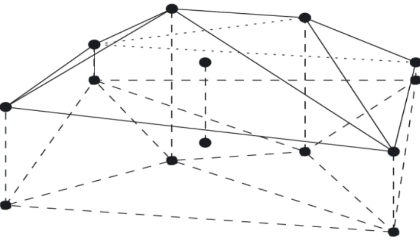
Figure 2.3: Tent-like structure for the logarithm of MLE when d = 2 (Figure from Cule et al. [2010])

Theorem 2.6. Suppose that f̂n is the univariate log-concave ML density estimator

of f0, then

dH( ̂fn, f0) =Op(n−2/5). (2.10)

2.3

Multi-dimensional log-concave density

2.3.1 Log-concave maximum likelihood estimation

In multivariate cases, the log-concave MLE was studied by Cule et al. [2010] and Cule [2009]. Cule et al. [2010] showed that with probability one, the log-concave ML

(49)

log-concave ML estimator is different from univariate log-log-concave ML estimator because we cannot write an objective function in the terms of slopes. Figure 2.3 shows an

example of a two-dimensional log-concave ML estimator in a log-scale. We can view this ML estimator as pulling a tent or a sheet in the vertical way, where the heights of the tent poles represent the values of logf̂n, which is built from bivariate data that are the black dots in the Figure. However, it will be harder to visualize when we deal with data more than two dimensions, because the illustrations are not obvious. LetX1, . . . , Xn be random samples fromf0 onRd and denoteCn=conv(X1, . . . , Xn) as a convex hull of data. According to Cule et al. [2010], an objective function for finding the ML estimator is

σ(y) = −1 n n ∑ i=1 yi+ ∫ Cn exp(¯hy(x))dx. (2.11)

Theorem 2.7. [Cule et al., 2010, Theorem 3] The function σ is a convex function. It has a unique minimum at y∗∈

Rn, say, and logf̂n=h¯y∗.

According to Cule et al. [2010], they called logf̂n as a ‘tent function’, which is a function ¯hy ∶ Rd →R for a fixed vector y = (y1, . . . , yn) ∈ Rn. ¯hy is a least concave function where

¯

(50)

2.3.2 A computational aspect of the multivariate log-concave ML esti-mator

The idea is to use Shor’s r-algorithm, which presented in Cule et al. [2010]. It is built for solving a convex and non-differentiable problems. This algorithm is to generate a sequenceyt_{, which} _σ(_yt) →_min

y∈_Rn

σ(y)as t→ ∞. σ(yt)_and _∂σ(_yt) _{will be} required at each iteration where ∂σ(yt) _{represents the direction moving from} _yt _to yt+1_.

Maximizing the multivariate log-concave objective function can be viewed as the

infinite dimensional optimization problem. It can be reduced to the problem of maximizing function ¯hy for some suitable vector y. In other words, we can imagine that the function ¯hy is when we place the pole height yi at Xi and pull the sheet over the top of the pole. Thus, a key for finding the log-concave ML estimator for multidimensional data is to find an appropriate vectory∗∈

Rn, wherey∗ _{comes from}

minimizing σ(y) in (2.11). From this minimization problem, we will get a unique y∗= (_y∗

1, . . . , y

∗

n) ∈Rn.

In order to calculate σ(y), we need to evaluate _∫_C

nexp(

¯

hy(x))dx. We can write the closed form of this integral by triangulating the convex hull of data, Cn. An example of the triangulations for d = 2 can be found in Figure 2.3. Each simplex represents an affine function of logf̂n. This step uses much computational time to

(51)

find a proper y∗ _{which makes ¯}_h

y∗ as a tent function that all tent poles touch the tent.

It can also be noticed that there is an available package in R that builts from Chen et al. [2015] for finding the multidimensional log-concave ML estimator. The package is calledLogConcDEADand the useful function is “mlelcd”. In this function,

the stopping criteria after the(r+1)th iteration are given by

∣yr+1 i −yri∣ ≤δ∣yri∣ for i=1, . . . , n, ∣σ(yr+1) − σ(yr)∣ ≤∣σ(yr)∣, ∣ ∫_C n exp ¯hyr(x)dx−1∣ ≤η,

for some small values of δ, , and η.

In the algorithm, these tolerances has been set toδ=10−4_,=₁₀−8_{, and} _η=₁₀−4_.

However, these stopping criteria can be set by a user in the mlelcd function with parameters ytol, sigmatol, and integraltol, respectively. An example code for finding the multivariate log-concave ML estimator by using theLogConcDEAD package is in

Appendix A.3.2.

2.3.3 Rate of convergence

Cule [2009] showed that the multivariate ML estimator f̂n is a consistent esti-mator of the true density f0. Moreover, they conjectured that the optimal rate of

(52)

convergence with respect to the Hellinger distance isn−2/(d+4)_.

Theorem 2.8. [Cule, 2009, Theorem 5.11] Let f0 be a log-concave density and let ̂

fn denote the log-concave maximum likelihood estimator. Then, with probability 1, dH( ̂fn, f0) →0 as n→ ∞.

Moreover, Cule [2009, page 97] conjectured that dH( ̂fn, f0) =Op(δn) where

δn= ⎧⎪⎪⎪ ⎪⎪⎪⎪⎪ ⎪⎪⎪⎪⎪ ⎨⎪⎪ ⎪⎪⎪⎪⎪ ⎪⎪⎪⎪⎪ ⎪⎩ n−2/(d+4) _when _d<₄_, n−1/4(_log_n)1/2 _when_d=₄_, n−1/d _when _d>₄_.

Then, they use the results from Cule [2009, Section 5.2.6] and conjectured that dH( ̂fn, f0) =Op(n−2/(d+4))for all d.

Furthermore, Kim and Samworth [2016, Theorem 5, page 2762] proved that the

actual rates of convergence for the log-concave ML estimator with respect to the Hellinger distance converges up to the logarithmic factors. However, they stated the results only for d≤3.

Theorem 2.9. [Kim and Samworth, 2016, Theorem 5, page 2762] Let X1, . . . , Xn

(53)

log-concave ML estimator. Then, dH( ̂fn,Fd) = ⎧⎪⎪⎪ ⎪⎪⎪⎪⎪ ⎪⎪⎪⎪⎪ ⎨⎪⎪ ⎪⎪⎪⎪⎪ ⎪⎪⎪⎪⎪ ⎪⎩ O(n−2/5) _if _d=₁_, O(n−1/3√_log_n) _if _d=₂_, O(n−1/4√_log_n) _if _d=₃

where Fd denote the set of upper semi-continuous, log-concave densities on Rd.

2.3.4 Computational time

As we mentioned before, the conjectured rate of convergence of the multivari-ate log-concave ML estimator is n−2/(d+4)_{, which is computationally intensive. The}

running time for four-dimensional data with sample size 1,000 is 18 minutes for a

1.60GHz/8GB RAM desktop PC. Unlike, for one-dimensional data, finding the ML estimator with the ASA in thelogcondens package takes under one second. Because it is a time-consuming algorithm, we propose a new method that works well with

multivariate density estimation and is also applicable in practice. This method will combine the knowledge of one-dimensional log-concave MLE with a copula model, which will be presented in the next Chapter.

(54)

3

Dependence modeling with copulas

3.1

Introduction

Because of the computationally intensive problem when we find the multivariate

log-concave ML estimator with Shor’sr-algorithm, we propose another useful method that works with the “copula model”. Copula can use to model the dependencies between variables and allows us to form a multivariate model in which its margins

are modeled separately from the dependence structure. We can find the estimators of each marginal density separately. Since our marginal densities are univariate log-concave densities, their ML estimators give us a better convergence rate than the

multivariate log-concave ML estimators. This is how the convergence rate can be improved.

Copula model has been widely used in several fields such as economics and finance,

see Patton [2012]. He applied the copula model with time series of the stock index returns and also presented the goodness of fit test for choosing an appropriate copula

(55)

family. R´emillard et al. [2012] presented the copula model with Archimedean copulas to work with the multivariate time series on the Canadian/US exchange rate and the

values of oil in the future ten-year period.

In this chapter, we show how to find the estimators under the copula model. The estimation can be done in two steps. First, we estimate the univariate log-concave

marginals. Then, we estimate the copula parameters. This two-stage estimation is called inference function for margins (IFM). As we mentioned before, univariate concave ML estimator gives the better rate of convergence than multivariate

log-concave ML estimator. Therefore, modeling under the copula model improves the performance of the density estimation in terms of the convergence rate. Moreover, it gaurantees that the convergence rate of our proposed method is much faster than

n−2/(d+4)_{, which is from the conjectured rate of multivariate log-concave ML}

esti-mator. However, our proposed rate is never better than the convergence rate of parametric estimator which is n−1/2_.

3.1.1 Definitions and properties

Copula is a multivariate function with uniform marginal distribution functions. Moreover, it can be called as a uniform representation or a dependence function,

(56)

concept of copula to work with ad-dimensional distribution functionF. We can split F into two parts, the marginal distribution functionsFj and the copula distribution functionC with its parameters θ∈_Rk_.

Definition 3.1. The joint distribution function F is a function with its domain in Rd which

F is nondecreasing.

F1, . . . , Fd are distribution functions.

F has marginsF1, . . . , Fdsuch thatFj(x) =F(∞, . . . , xj, . . . ,∞)forj=1, . . . , d.

F(x1, . . . ,−∞, . . . , xd) = 0 especially for d =2. F(x,−∞) = F(−∞, y) = 0 and F(∞, . . . ,∞) =1.

Theorem 3.2. (Sklar’s theorem) Let X= (X1, . . . , Xd)be a random vector with

dis-tribution function F and F ∈ F(F1, . . . , Fd) be a d-dimensional distribution function

with margins F1, . . . , Fd. Then there exists a d-copula C with uniform margins such

that

F(x1, . . . , xd) =C(F1(x1), . . . , Fd(xd)). (3.1)

(57)

cop-uniform random vector [Joe, 1997]. Note that a copula,C, is defined as a cumulative distribution function with support in [0,1]d_{. Moreover, a copula density function of} the copula distribution function C is given by

c(F1, . . . , Fd) =

∂d_C(_F

1, . . . , Fd) ∂F1⋯∂Fd

. (3.2)

Furthermore, some properties of C are as follows.

1. The copula function is always unique if all marginal functions are continuous. Conversely, if C is a d-copula with distribution function F1, . . . , Fd, then F from (3.1) is ad-dimensional distribution function with margins F1, . . . , Fd.

2. For Fj ∈ [0,1];j =1, . . . , d, when ∂dC(F1, . . . , Fd)/(∂F1⋯∂Fd) exists, C is ab-solutely continuous.

3. Every copula C is continuous and satisfies the following inequality

∣C(F1, . . . , Fd)−C(G1, . . . , Gd)∣ ≤ ∑dj=1∣Fj−Gj∣when∀1≤j≤d, and 0≤Fj, Gj ≤

1.

4. For all 1≤j ≤d, 0≤Fj ≤1, we have Cj(Fj) =C(1, . . . ,1, Fj, . . . ,1, . . . ,1) =Fj and Cj(Fj) =C(F1, . . . ,0, . . . , Fj, . . . , Fd) =0.

5. If g1, . . . , gd are monotone, nondecreasing mappings of R in itself, any copula function of(X1, . . . , Xd) is also a copula function of (g1(X1), . . . , gd(Xd)).

(58)

6. For a bivariate copula, there are some interesting properties as follows.

C(1, u) =C(u,1) =u and C(0, u) =C(u,0) =0 for all u∈ [0,1].

C is nondecreasing in each variable.

For every s, t, u, v∈ [0,1], such that s≤t and u≤v, then

C(t, v) −C(t, u) −C(s, v) +C(s, u) ≥0.

For every s, t, u, v∈ [0,1], C satisfies the following Lipschitz condition

∣C(t, v) −C(s, u)∣ ≤ ∣t−s∣ + ∣v−u∣.

Moreover, copulas have their universal bound called “Fr´echet-Hoeffding bounds inequality” as given in Theorem 3.3.

Theorem 3.3. Let C be any d-copula with F1, . . . , Fd be marginal distribution

func-tions with support in [0,1]d_{. Then,}

W(F1(x1), . . . , Fd(xd)) ≤ C(F1(x1), . . . , Fd(xd)) ≤ M(F1(x1), . . . , Fd(xd))

where W(F1(x1), . . . , Fd(xd)) =max(F1(x1) + ⋅ ⋅ ⋅ +Fd(xd) −d+1,0) and

M(F1(x1), . . . , Fd(xd)) =min(F1(x1), . . . , Fd(xd)). Moreover, an independence

(59)

Figure 3.1: Graphics of M, W, and Π (figure from Nelsen [2006])

W and M are called lower and upper Fr´echet-Hoeffding bounds. The copula

C(F1(x1), . . . , Fd(xd)) =M(F1(x1), . . . , Fd(xd)) represents the most positive depen-dence. The functionsM and Π ared-copulas for all d≥2. On the other hand, W is a copula only whend≤2. WhenC(F1(x1), . . . , Fd(xd)) =max(F1(x1) + ⋅ ⋅ ⋅ +Fd(xd) − d+1,0), it represents the most negative dependence. Furthermore when X1, . . . , Xd are independent,C(F1(x1), . . . , Fd(xd)) =Π(F1(x1), . . . , Fd(xd)) =F1(x1)⋯Fd(xd).

3.1.2 Dependence

For a set of distributions F(F1, . . . , Fd), there are several statistics for measuring the level of dependences between random variables. In our work, we first discuss concordance. Then, we present two famous measures, which are Spearman’s rho and

(60)

Kendall’s tau.

3.1.2.1 Concordance

The random variables with distribution function F and Gare said to be concor-dant if the large values of F are associated with the large values of G and also the small values of F and Gare being small together.

Definition 3.4. (Concordance) LetF andGbe distribution functions inF(F1, . . . , Fd) whereX∼F, Y ∼GandX, Y are continuous random variables such that(xi, yi)and

(xj, yj) are the two observations from a vector (X, Y). Then, (xi, yi) and (xj, yj) are concordant if xi >xj and yi >yj orxi <xj and yi <yj. Conversely, we say that they are discordant when xi >xj but yi <yj or if xi <xj and yi >yj. The formula can be represented as(xi−xj)(yi−yj) >0 for concordance and(xi−xj)(yi−yj) <0 for discordance.

Theorem 3.5. [Nelsen, 2006, Theorem 5.1.1] Let (X1, Y1) and(X2, Y2) be

indepen-dent vectors of continuous random variables with joint distribution functionsH1 and

H2, respectively, with common margins F (of X1 and X2) and G (of Y1 and Y2).

Let u=F(x), v=G(y), and C1 and C2 denote the copulas of (X1, Y1) and (X2, Y2),

respectively, so that H1(x, y) =C1(F(x), G(y)) and H2(x, y) =C2(F(x), G(y)). Let

(61)

(X1, Y1) and (X2, Y2), i.e., let Q=P[(X1−X2)(Y1−Y2) >0] −P[(X1−X2)(Y1−Y2) <0]. Then, Q=Q(C1, C2) =4∫ 1 0 ∫ 1 0 C2(u, v)dC1(u, v) −1. 3.1.2.2 Spearman’s rho

Spearman’s rho correlation is based on both concordance and discordance. We

will show details of this correlation via examples of three independent random vec-tors. Let (X1, Y1),(X2, Y2),(X3, Y3) be three independent random vectors from a

joint distribution functionH whereF andGare the marginal distribution functions of X and Y, respectively. The Spearman’s rho for (X1, Y1) and (X3, Y2) is given by

ρC =3{P[(X1−X3)(Y1−Y2) >0] −P[(X1−X3)(Y1−Y2) <0]}. (3.3)

The equation (3.3) represents a probability of concordance minus a probability of

discordance times a normalizing constant. Note that we can also use(X2, Y3)instead

of(X3, Y2). The idea is that one vector has the joint distribution function H, which

is(X1, Y1), and another vector (X3, Y2)is independent. Thus, the joint distribution

(62)

Y2 are independent, the copula of(X3, Y2)is Π. Then from Theorem 3.5, we get Q(C,Π) =4_∫ 1 0 ∫ 1 0 uv dC(u, v) −1. (3.4)

The Spearman’s rho can also be viewed as the measurement of how far from inde-pendent of the variables. To study the range ofQ(C,Π), we work on the boundaries of (3.4). The lower and upper bounds ofQ(C,Π) are given by

Q(W,Π) =4_∫ 1 0 ∫ 1 0 uv dW(u, v) −1, and Q(M,Π) =4_∫ 1 0 ∫ 1 0 uv dM(u, v) −1.

Because the support ofW is the second diagonal G(y) =1−F(x), therefore

∫ 1 0 ∫ 1 0 h(u, v)dW(u, v) = ∫ 1 0 h(u,1−u)du (3.5)

for all integrable function h, which domain is in [0,1]2_{. Likewise, the support of} _M

is the main diagonal G(y) =F(x) in[0,1]2_{. Because}_M _{has a uniform margin, then}

∫ 1 0 ∫ 1 0 h(u, v) dM(u, v) = ∫ 1 0 h(u, u) du. (3.6) Therefore, we have Q(W,Π) =4_∫ 1 0 u(1−u)du−1= −1 3 and Q(M,Π) =4_∫ 1 0 u2 du−1= 1 3.

Consequently, for any copula C, Q(C,Π) ∈ [−1/3,1/3]. A multiplier 3 in (3.3) is

(63)

Theorem 3.6. [Nelsen, 2006, Theorem 5.1.6] Let X and Y be continuous random variables whose copula is C. Then the population version of Spearman’s rho for X

and Y is given by ρC = 3Q(C,Π) = 12_∫ 1 0 ∫ 1 0 uv dC(u, v) −3 = 12_∫ 1 0 ∫ 1 0 C(u, v) dudv−3 = 12_∫ 1 0 ∫ 1 0 {C(u, v) −uv}dudv.

Example 3.7. Farlie-Gumbel -Morgenstern (FGM) copula

C(u, v) =uv+θuv(1−u)(1−v); θ∈ [−1,1], (3.7) then ρC = 12∫ 1 0 ∫ 1 0 { uv+θuv(1−u)(1−v) −uv}dudv = 12(1 6) ∫ 1 0 θv(1−v) dv = θ 3. Hence, ρC ∈ [−1/3,1/3]. 3.1.2.3 Kendall’s tau

A population version of Kendall’s tau is also related to the concordance and

(64)

distributed random vectors from the same joint distribution function H. Therefore, the population version of Kendall’s tau is in the form of

τC =P[(X1−X2)(Y1−Y2) >0] −P[(X1−X2)(Y1−Y2) <0]. (3.8)

Theorem 3.8. [Nelsen, 2006, Theorem 5.1.3] Let X and Y be continuous random variables whose copula is C. Then, the population version of Kendall’s tau for X

and Y is given by τC = Q(C, C) = 4_∫ 1 0 ∫ 1 0 C(u, v) dC(u, v) −1 = 4_∫ 1 0 ∫ 1 0 C(u, v)c(u, v) dudv−1.

The lower and upper bounds of Q(C, C) can be calculated from Q(W, W) and Q(M, M), respectively. We use the calculations in (3.5) and (3.6), hence we get

Q(W, W) =4_∫ 1 0 ∫ 1 0 max(u+v−1,0)dW(u, v) −1 =4_∫ 1 0 0du−1= −1, Q(M, M) =4_∫ 1 0 ∫ 1 0 min(u, v)dM(u, v) −1 =4_∫ 1 0 u du−1=1. Therefore,Q(C, C) ∈ [−1,1].

(65)

Example 3.9. Farlie-Gumbel -Morgenstern (FGM) copula Refer to the FGM copula distribution function in (3.7), we get

∂uC(u, v) =v+θv(1−v)(1−2u) ∂u∂vC(u, v) =1+θ(1−2u)(1−2v) =c(u, v). Then, τC =4∫ 1 0 ∫ 1 0 { uv+θuv(1−u)(1−v)} {1+θ(1−2v)(1−2u)}dudv−1 =4(1 4+ θ 18) = 2θ 9 .

Because of θ ∈ [−1,1], therefore τC ∈ [−2/9,2/9]. According to Example 3.7 and 3.9, FGM has restricted usefulness because ρC and τC have the limited ranges of dependence.

Although, both Spearman’s rho (ρ) and Kendall’s tau (τ) are the measurements of dependence. There are some differences. First, the range of dependence that ρC

and τC can cover are different as shown in Example 3.7 and 3.9. Second, Nelsen

[2006] showed universal inequality for these two measures.

Theorem 3.10. [Nelsen, 2006, Theorem 5.1.10] LetX andY be continuous random variables, and letρ and τ denote Spearman’s rho and Kendall’s tau, defined by (3.3)

and (3.8), respectively. Then,

(66)

3.1.3 Copula families

In this thesis, we focus on parametric copula families. However, there are also nonparametric copulas such as empirical copula and kernel copula. Some parametric

copula families contain one parameter. Some contain more than one parameter, see Durrleman et al. [2000], Nelsen [2006] and Yan [2007]. We show some examples of bivariate Gaussian and Archimedean copula families. Gaussian copula has one

parameter but Archimedean copulas contain both one parameter and two parameters families. In each example, we present the copula distribution function, the copula

density that derives from the representation in (3.2), and also the explicit form of Spearman’s rho and Kendall’s tau if they can be shown explicitly. For examples below, let u, v be the uniform representations of F(x) and G(y).

3.1.3.1 Gaussian copula

C(u, v) =Nθ(Φ−1(u),Φ−1(v)); u, v∈ (0,1)

The bivariate Gaussian copula density function can be represented as

c(u, v) = √ 1 detRexp ⎛ ⎜⎜ ⎜⎜ ⎝ −1 2 ⎡⎢ ⎢⎢ ⎢⎢ ⎢⎢ ⎣ Φ−1(_u) Φ−1(_v) ⎤⎥ ⎥⎥ ⎥⎥ ⎥⎥ ⎦ T (R−1− I) ⎡⎢ ⎢⎢ ⎢⎢ ⎢⎢ ⎣ Φ−1(_u) Φ−1(_v) ⎤⎥ ⎥⎥ ⎥⎥ ⎥⎥ ⎦ ⎞ ⎟⎟ ⎟⎟ ⎠ .

(67)

Let consider the correlation matrix R= ⎡⎢ ⎢⎢ ⎢⎢ ⎢⎢ ⎣ 1 θ θ 1 ⎤⎥ ⎥⎥ ⎥⎥ ⎥⎥ ⎦

where det(R) =1−θ2_{, then}

R−1− I = 1 1−θ2 ⎡⎢ ⎢⎢ ⎢⎢ ⎢⎢ ⎣ 1 −θ −θ 1 ⎤⎥ ⎥⎥ ⎥⎥ ⎥⎥ ⎦ − ⎡⎢ ⎢⎢ ⎢⎢ ⎢⎢ ⎣ 1 0 0 1 ⎤⎥ ⎥⎥ ⎥⎥ ⎥⎥ ⎦ = θ 1−θ2 ⎡⎢ ⎢⎢ ⎢⎢ ⎢⎢ ⎣ θ −1 −1 θ ⎤⎥ ⎥⎥ ⎥⎥ ⎥⎥ ⎦ . Therefore, c(u, v) = √ 1 1−θ2 exp ⎛ ⎜⎜ ⎜⎜ ⎝ −1 2( θ 1−θ2) ⎡⎢ ⎢⎢ ⎢⎢ ⎢⎢ ⎣ θΦ−1(_u) −_Φ−1(_v) −Φ−1(_u) +_θ_Φ−1(_v) ⎤⎥ ⎥⎥ ⎥⎥ ⎥⎥ ⎦ T ⎡⎢ ⎢⎢ ⎢⎢ ⎢⎢ ⎣ Φ−1(_u) Φ−1(_v) ⎤⎥ ⎥⎥ ⎥⎥ ⎥⎥ ⎦ ⎞ ⎟⎟ ⎟⎟ ⎠ = √ 1 1−θ2 exp(− θ 2(1−θ2)[θ(Φ −1( u))2−2Φ−1( u)Φ−1( v) +θ(Φ−1( v))2]).

Kendall’s tau is given by

τ = 2

πarcsin(θ), where θ is the Spearman’s rho.

3.1.3.2 The t copula Letx= (x1, x2)T, C(u, v) = ∫ t−1 δ (u) −∞ ∫ t−1 δ (v) −∞ Γ(δ+2 2 ) Γ(δ₂)πδ√1−θ2(1+ xT_R−1_x δ ) −(δ+2)/2 dx,

(68)

wheret−1

δ denote the quantile function of a standard univariatetδ distribution withδ degrees of freedom, andR is the correlation matrix with off-diagonal elements equal toθ. The density of t copula has a form

c(u, v) = fδ,θ(t −1 δ (u), t −1 δ (v)) fδ(t−_δ1(u))fδ(t−_δ1(v)) ;u, v∈ (0,1),

wherefδ,θ is the joint density of bivariate standard t-distributed random vectors and fδ is the standardt density function with degrees of freedom δ. Thetcopula has the same Spearman’s rho and Kendall’s tau as the Gaussian copula.

3.1.3.3 Archimedean copulas

Let φ[−1] _{denote a pseudo-inverse of} _φ _{and considers} _φ _{as a continuously strictly}

decreasing convex function from[0,1]to[0,∞]. The functionφ is called a generator of the copula. Thus, we have

φ[−1]( t) = ⎧⎪⎪⎪ ⎪⎪⎪⎪ ⎨⎪⎪ ⎪⎪⎪⎪⎪ ⎩ φ−1(_t) _for _t∈ [₀_{, φ}(₀)]_, 0 for t≥φ(0).

Note thatφ[−1] _{is continuous and nonincreasing on} [₀_,∞] _{but strictly decreasing on}

[0, φ(0)]. The distribution function of Archimedean copula is given by

C(u, v) =φ[−1](

(69)

We say that C is strict, when φ(0) = ∞ and C(u, v) > 0 for all (u, v) ∈ [0,1]2_.

On the contrary, C is non-strict when φ(0) < ∞. When the copula C is strict, φ[−1] = _φ−1_{. The copula in (3.9) is said to be a strict Archimedean copula, which}

equals to φ−1(_φ(_u) +_φ(_v))_{. Kendall’s tau of the Archimede}