Developing Risk of Mortality and
Early Warning Score Models
using Routinely Collected Data
by
Tessy Badriyah
The thesis is submitted in partial fulfilment of the requirements for the award of the degree of Doctor Philosophy of the University of Portsmouth
Abstract
Aim. The aim of this study was to contribute to the building of effective and efficient methods to predict adverse clinical outcome. It has been done by developing risk of mortality and early warning score models using routinely collected data that are available from hospital computer systems.
Methods. To predict risk of mortality, firstly we used logistic regression using (Biochemistry and Haematology Outcome Model - BHOM dataset) to generate a model, and the performance of each model was then compared using discrimination (AUROC or c-index) and calibration (the Hosmer-Lemeshow test). Secondly, we focused on decision trees (DT) to be compared with logistic regression (LR). In addition, we used cross validation to compare LR with other various machine learning methods. We developed early warning score algorithmically using decision trees (DTEWS) using vital sign dataset and compared the performance of DTEWS with other EWSs based on clinical expertise using c-index, early warning score efficiency curve and distribution score. We also compared DTEWS with another EWS based on statistics and applied DTEWS to BHOM dataset.
Results. In BHOM dataset, there were 9497 adult hospital discharges, and it was divided into four subsets. A model was built using one training set and then applied to three other testing data sets. The model in logistic regression satisfied both discrimination and calibration value when the c-index in the range 0.700-0.800 is reasonable discrimination and the p-value > 0.05 indicates there is no evidence of significant lack of fit. We also found that decision trees gave a satisfactory result followed by some other machine learning methods.Using a large vital signs dataset (n = 198,755 observation sets) from acute medical admissions, DTEWS can provide a discrimination (c-index) as good as other EWSs, has a better c-index, and also is better in other measurements including EWS efficiency curve, and distribution of score. We found DTEWS can also be applied to BHOM dataset with satisfactory results.
Conclusion. The results of this study support the idea that decision trees can be applied to medical problems. When we produced a model for risk of mortality, we have shown that the decision trees model has reasonable discrimination and could be considered as an alternative technique to logistic regression. We have shown that a structured methodology using decision trees to develop early warning score has satisfactory result and contributes additional evidence that suggests an algorithmical method can be employed to quickly produce EWSs for employment in particular types of medical purpose.
Declaration of authorship
Whilst registered as a candidate for the above degree, I have not been registered for any other research award. The results and conclusions embodied in this thesis are the work of the named candidate and have not been submitted for any other academic award.
... TESSY BADRIYAH
Table of Contents
Abstract i
Declaration of authorship ii
Table of Contents iii
List of Tables vii
List of Figures x
Abbreviation xii
Acknowledgement xiii
Dissemination xiv
Chapter 1 Introduction ... 1
1.1 Background to the research ... 1
1.2 The aim of the study ... 5
1.3 The rationale for this study ... 6
Chapter 2 Literature Review ... 12
2.1 Extracting useful knowledge from the data ... 13
2.1.1 Data definition and collection 15 2.1.2 Knowledge discovery from data 17 2.2 Classification and Prediction ... 19
2.2.1 Classification by Decision Trees Induction 21 2.2.2 Transformation of a decision tree into decision rules 29 2.2.3 Pruning to overcome the limitation of decision trees 30 2.2.4 Handling continuous attribute values in decision trees 32 2.2.5 Handling unknown (missing) values in decision trees 33 2.3 Prediction by regression methods ... 33
2.3.1 Simple linear regression and correlation 34 2.3.2 Multiple regression 36 2.3.3 Logistic regression 37 2.3.4 Which regression method do we need to use? 38 2.4 Assessing performance of a model ... 39
2.4.1 Accuracy (accuration rate) 40
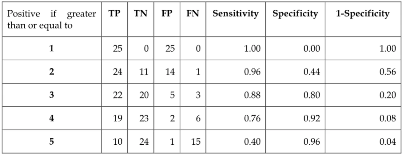
2.4.2 Sensitivity, Specificity, and precision 43
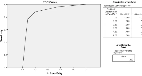
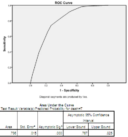
2.4.3 Area under ROC Curves 46
2.4.4 Using p-values and confidence intervals to interpret results 51
2.4.5 Calibration using chi-square statistic 54
2.4.6 Statistical inference to evaluate the differences between two
2.5 Re-sampling method ... 60
2.6 A brief history of physiological outcome modelling ... 62
2.6.1 The history 62 2.6.2 Logistic regression is the most popular method to predict risk of mortality 64 2.6.3 Developing risk of mortality using methodology in machine learning 65 2.7 Recognising and responding to clinical deterioration ... 66
2.7.1 Systems for recognising and responding to clinical deterioration 67
2.7.2 Rapid Response System: recognising and responding to clinical deterioration 68 Chapter 3 Developing a model of risk of mortality using routinely collected data ... 72
3.1 Introduction ... 72
3.2 Design of a System to Predict Clinical Outcomes ... 73
3.3 Ethical Considerations ... 74
3.4 Data Description ... 75
3.5 The characteristics of the dataset ... 76
3.6 Assessing performance of a model ... 77
3.6.1 Discrimination using area under ROC curve (AUROC) 77 3.6.2 Calibration using chi-test 78 3.6.3 Exhaustive method 79 3.6.4 t-test statistics to assess models from cross validation 80 3.7 Developing a Risk of Mortality Model using SPSS ... 81
3.7.1 Logistic Regression Model 81 3.7.2 Decision Trees Model 88 3.7.3 The effects of changes of the type of data in the independent attributes 94 3.7.4 Discussion of the Results 96 3.8 Developing a risk of mortality model using MATLAB ... 98
3.8.1 Logistic regression model 98 3.8.2 Decision Trees Model 101 3.8.3 Implementation of stratification model and calibration using chi-test 105 3.8.4 Implementation of Exhaustive method to assess performance of the model 111 3.8.5 Discussion of the Results 113 3.9 Developing a risk of mortality model using RapidMiner ... 115
3.10 Cross Validation ... 117
3.10.1 Generate Dataset for Cross-Validation 118 3.10.2 Cross Validation among methods in Machine Learning 119 3.11 The summary of results and overall discussion ... 122
Chapter 4 A Structured methodology for developing early warning score using decision trees (DTEWS) ... 125 4.1 Introduction ... 125 4.2 Previous Study ... 126
4.2.1 The characteristics of the dataset 126
4.2.2 The method to develop early warning score 128
4.2.3 The performance 129
4.3 Methodology to generate early warning score ... 129
4.3.1 Data used and Description 129
4.3.2 Assessing performance of a model 131
4.4 A new structured methodology to develop early warning
score using decision trees (DTEWS) ... 134 4.5 Develop early warning score using MATLAB ... 138
4.5.1 Illustration of DTEWS methodology 138
4.5.2 Decision trees model and generating cut points 139
4.5.3 Building tree table 141
4.5.4 Generating Score 143
4.5.5 Determine weighting scores 145
4.5.6 Building early warning score system 146
4.6 Evaluation of DTEWS methodology ... 147 4.6.1 Comparing score values and the performance 148 4.6.2 Evaluating the efficiency using EWS efficiency curve 150 4.6.3 Distribution score for different age groups 152 4.7 Extending DTEWS ... 153
4.7.1 Score using multiple % (percentage of death) 154
4.7.2 Using relative risks 159
4.7.3 Using different thresholds 160
4.7.4 Using different number of risk bands 162
4.8 The summary of results and overall discussion ... 165 Chapter 5 Validating and Comparing decision tree early warning score (DTEWS) 168
5.1 Introduction ... 168 5.2 DTEWS validates National Early Warning Score (NEWS) ... 169
5.2.1 Minor changes between ViEWS and NEWS 169
5.2.2 Data used and description 171
5.2.3 Generating score from 4 other adverse clinical outcomes 173
5.2.4 Comparing performance amongs EWSs 175
5.3 Comparing DTEWS with other system based on statistics
(Centile) ... 182 5.3.1 Generating score of vital sign dataset using Centile 182 5.3.2 Comparing score values between DTEWS and Centile 187 5.4 Modelling BHOM dataset using DTEWS methodology ... 192 5.5 The summary of results and overall discussion ... 194
Chapter 6 Overall Discussion and Conclusion ... 196
6.1 Study Outcome ... 196
6.2 Original Contribution to Knowledge and limitation of the study ... 200
6.3 Reflection on the Results in Clinical Context ... 201
6.4 Suggestions for future work ... 202
6.5 Overall conclusion ... 202 Appendices 204
List of Tables
Table 2.1 Dataset Hypertension 16
Table 2.2 Hypertension dataset 24
Table 2.3 Hypertension dataset, comparing predicted and observed
value 41
Table 2.4 Confusion matrix for three classes 43
Table 2.5 Sample dataset to demonstrate area under ROC curve 48 Table 2.6 Set of points in the Sensitivity and 1-Specificity to form ROC
curve 49
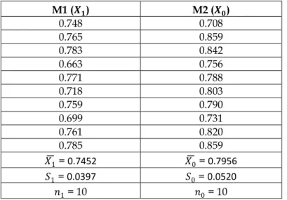
Table 2.7 Predicted and observed risks in bands 55 Table 2.8 c-index obtained from applying two methods, using 10-fold
cross validation 58
Table 3.1 The performance of model when validating other datasets 87 Table 3.2 The performance of Decision Trees model when validating
other datasets 94
Table 3.3 Comparison discrimination between Logistic Regression
and Decision Trees model using SPSS 96
Table 3.4 The performance of the logistic regression model using
MATLAB when validating other datasets 101
Table 3.5 The performance of Decision Trees model using MATLAB
when validating other datasets 105
Table 3.6 Stratification of Logistic Regression Model using SPSS,
based on Equation 3.1/ Equation 3.2 108
Table 3.7 Stratification of Logistic Regression Model using SPSS by
Prytherch, et.al. (2005) 109
Table 3.8 Stratification of Logistic Regression model using MATLAB 109 Table 3.9 Stratification model of Logistic Regression model using
SPSS and MATLAB 110
Table 3.10 Stratification model of Decision Trees model using SPSS
and MATLAB 110
Table 3.11 Performance of discrimination, calibration and exhaustive method of Logistic Regression model using SPSS and
MATLAB 112
Table 3.12 Performance of c-index, χ2 (chi-test) and exhaustive
method of decision trees model using SPSS and MATLAB 113 Table 3.13 Comparison Stratified Modelling by
RapidMinerFrameWork using Q1 as training data,
Q2,Q3,Q4 as testing data 116
Table 3.14. The performance of six (6) methods in subset1 formed
10-fold cross validation. 120
Table 3.15 The performance of LR to be compared with 5 other
methods (DT, SVM, NB, NN, KNN) using t-test statistics. 121 Table 4.1 The characteristics of the patients in the study 127
Table 4.2 ViEWS early warning score by (Prytherch, et al., 2010) 128
Table 4.3. Tree table for heart rate variable 135
Table 4.4 Converting percentage of death into the score for heart rate
variable 136
Table 4.5 Score for heart rate variable 136
Table 4.6 Decision trees SPSS early warning score using vital signs1
dataset 137
Table 4.7 Tree table for Heart rate field 142
Table 4.8 Generating score for heart rate variable 143 Table 4.9 Tree table and generating score for temperature variable 144 Table 4.10 Score for heart rate variable in MATLAB 145 Table 4.11 DTEWS early warning score using vital signs1 dataset 146 Table 4.12 Research question and expected answer 147 Table 4.13 Sensitivity and Specificity that performing ROC curve for
ViEWS and DTEWS 148
Table 4.14 EWS Efficiency curve between ViEWS and DTEWS 150 Table 4.15 Tree table and generating score for heart rate variable using
vital sign2 dataset 154
Table 4.16 Different scoring system between score 0-3 and actual score 155 Table 4.17 Weighting score for heart rate variable in vital signs2 dataset
using score 0-3 155
Table 4.18 Weighting score for heart rate variable in vital signs2 dataset
using multiple % (percentage of death) 156
Table 4.19 Early warning score of vital sign2 dataset using score 0,1,2,3
and score using actual percentage 156
Table 4.20 Different performance of c-index between two different
scores using vital sign2 dataset 157
Table 4.21 Tree table and generating score for heart rate variable using
vital sign3 dataset using actual percentage 158
Table 4.22 Tree table and generating score for heart rate variable using
vital sign3 dataset using relative risks 159
Table 4.23 Different threshold scores of DTEWS on vital sign1 dataset (using score 0,1,2,3 and score 0, 2, 4, 6) 160 Table 4.24 The performance of early warning score using different
threshold 161
Table 4.25 vital signs1 dataset, score 0-1 162
Table 4.26 vital signs1 dataset, score 0-2 163
Table 4.27 vital signs1 dataset, score 0-4 163
Table 4.28 The performance of different number of risk bands to
generate early warning scores using vital sign1 dataset 164 Table 5.1 Comparison of early warning score of ViEWS and NEWS 170 Table 5.2 Four others adverse clinical outcomes dataset and the
percentage of death 172
Table 5.3 Early warning score for any of 3 other adverse clinical
Table 5.4 Early warning score for death with precedence
(DEATH_PRECEDENCE dataset) 174
Table 5.5 Early warning score for unanticipated ICU admission
precedence (ITU_PRECEDENCE dataset) 174
Table 5.6 Early warning score for cardiac arrest precedence
(CA_PRECEDENCE dataset) 175
Table 5.7 The area under ROC curve (c-index) amongs ViEWS,
DTEWS and NEWS using vital sign1 dataset 176 Table 5.8 The area under ROC curve for 4 other adverse clinical
outcomes amongs 3 EWS scores 179
Table 5.9 Weighting scores for heart rate variable using Centile 185 Table 5.10 Centile early warning score using vital signs1 dataset 186 Table 5.11 The area under ROC curve (c-index) amongs ViEWS,
DTEWS and NEWS using 4 other adverse clinical outcomes
datasets 190
Table 5.12 Generating score for wcc variable using CART method 192 Table 5.13 Generating score for wcc variable using CHAID method 193 Table 5.14. Early warning score for BHOM dataset 193 Table 5.15 Discrimination of BHOM model developed by DTEWS
List of Figures
Figure 2.1 Decision Tree for hypertension dataset 21 Figure 2.2 Split at the root node of the decision tree 25 Figure 2.3 Transformation of a decision tree into decision rules 30 Figure 2.4 The intercept and slope of the regression equation 35 Figure 2.5 A confusion matrix for positive and negative records 42
Figure 2.6 ROC Curve from table 2.8 49
Figure 2.7 ROC curve, cut-off values and calculation of area under the
curve using SPSS 50
Figure 2.8 The approximate normal curve describing the distribution
of height of adult men 53
Figure 3.1 Design of System to Predict Clinical Outcome 74 Figure 3.2 Generate Logistic Regression Model using SPSS 82
Figure 3.3 Variables in the Equation Output 83
Figure 3.4 Categorical Variables Codings output 83 Figure 3.5 Developing syntax to calculate the probability attribute 84 Figure 3.6 Generate area under ROC curve for Logistic Regression
model 85
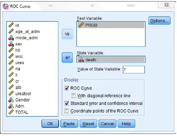
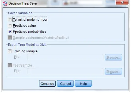
Figure 3.7 Area under ROC curve for Q1 dataset model 86 Figure 3.8 Generate Decision Trees model using SPSS 88 Figure 3.9 The option to save predicted probabilities in Decision Trees
model 89
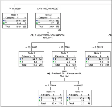
Figure 3.10 Complete Decision Trees model 90
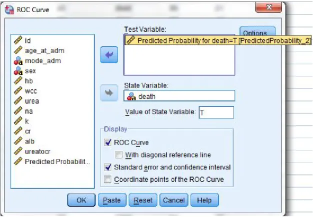
Figure 3.11 Zoom-out from Decision Trees model in Figure 3.10 90 Figure 3.12 Generate area under ROC curve for Decision Trees model 91 Figure 3.13 Area under ROC curve for Q1 dataset using Decision Trees
model 92
Figure 3.14 Saving Decision Trees model 93
Figure 3.15 Decision trees model produced by MATLAB 106 Figure 3.16 Main Process in RapidMiner’s framework 115 Figure 4.1 Early Warning Score efficiency curve comparison amongs
EWS score by (Prytherch, et al., 2010), (Subbe, et al., 2001)
and (Allen, 2004) 132
Figure 4.2 The distribution of VIEWS score (Prytherch, et al., 2010)
and associated mortality 133
Figure 4.3 Decision trees model for heart rate variable 134 Figure 4.4 Illustration of DTEWS process when it generates EWS for
each variable 139
Figure 4.5 Decision trees for heart rate (pulse) variable 140 Figure 4.6 Area under ROC curve (c-index) between ViEWS and
DTEWS 149
Figure 4.7 the EWS efficiency curves for DTEWS and NEWS using
Figure 4.8 Distribution of scores generated by VIEWS and DTEWS and associated mortality within 24h of a given vital signs
observation set using vital signs1 dataset 152 Figure 4.9 Percentage deaths by ViEWS & DTEWS score for each age
group 153
Figure 5.1 The area under ROC curve (c-index) amongs ViEWS,
DTEWS and NEWS using vital sign1 dataset 176 Figure 5.2 Distributed score of ViEWS, DTEWS and NEWS on vital
sign1 dataset 177
Figure 5.3 EWS efficiency curve between DTEWS and NEWS on vital
sign1 dataset 178
Figure 5.4. EWS efficiency curve between ViEWS and NEWS on vital
sign1 dataset 178
Figure 5.5 The comparison of the area under ROC curve among 3
EWS scores on 4 other adverse clinical outcomes 179 Figure 5.6 Distribution of scores of ViEWS, DTEWS and NEWS on 4
other clinical outcomes dataset 180
Figure 5.7 EWS efficiency curve of ViEWS, DTEWS and NEWS on 4
other adverse clinical outcome dataset 181
Figure 5.8 Generate Centile score 183
Figure 5.9 Choose heart rate variable as an example 184
Figure 5.10 Deciding perCentile 184
Figure 5.11 Obtained percentile scores 185
Figure 5.12 Comparison between AUROC of DTEWS and Centile 187 Figure 5.13 Distribution of score between DTEWS and Centile 188 Figure 5.14 Comparison of EWS efficiency curve between DTEWS and
Centile 188
Figure 5.15 Area under ROC curve (c-index) between DTEWS and
CENTILE using 4 adverse clinical outcome datasets 189 Figure 5.16 Distribution score of DTEWS and CENTILE using 4 other
adverse clinical outcome datasets 190
Figure 5.17 EWS efficiency curve between DTEWS and CENTILE using 4 other adverse clinical outcome datasets 191
Abbreviation
AI: Artificial Intelligence
AWTTS: Aggregate Weighted Scoring Systems
BP_SYS: Blood pressure systolic
BP_DIA: Blood pressure diastolic
CA: cardiac arrest
CART: Classification Regression Trees
CHAID: Chi-Square Automatic Interaction Detector
CONC_LEVEL: Conscious Level
DM: Data Mining
DT: Decision Trees
EWS: Early Warning Score
HR: Heart Rate
ITU: unanticipated ICU admission
KNN: K-Nearest Neighbours
LR: Logistic Regression
ML: Machine Learning
NB: Naïve Bayes
NEWS: National Early Warning Score
NN: Neural Networks
RCP: Royal College of Physicians
SVM: Support Vector Machines
UK: United Kingdom
Acknowledgement
First of all, all praises and thanks to Allah - God Almighty. It is so much blessing that I can present this thesis. And special thanks must go to my family, my husband, Iwan Syarif, my children Daisy, Defita and Pascal, my Dad and my Mum, Makhmud Mujab and Ilik Mizan, this work dedicated to you, thanks so much for all supports and never ending love for me.
I thank to my first supervisor, Dr. Jim Briggs who gives all the guidance, for his support in which ever form without which I possibly wouldn’t have been able to achieve this. I sincerely appreciated it.
I would especially like to thank Dr. Tineke Fitch for her support in all those ways could make me have the opportunity to come and study in the UK. I thank to my second supervisor Prof. Dave Prytherch for guidance and provision of data used in this study, my third supervisor Dr. Ivan Jordanov for discussion in the early of my study, and also Mrs. Deborah Prytherch, for the great proofreading and editing.
I thank to my PhD committee, Dr. Mohamed Gaber, Dr. Christine Urquhart and Dr. Chris Subbe for their valuable inputs and suggestions on my Thesis during my VIVA on 6th September 2013.
I thank to Prof. Gary Smith for provision of data and publishing paper, Dr. M Mohammed for useful advice and also all member of clinical outcome modelling team for cooperation. I would like to take this opportunity of thanking to all my colleagues in Electronic Engineering Polytechnic Institute of Surabaya (EEPIS) and all staff in the School of Computing, University of Portsmouth, thank you for your support. To all my friends, and all my fellow PhD students in the department, thank you for your support and friendship. I am indebted to the Indonesian Government for the scholarship for my PhD study for 3.5 years and also School of Computing, University of Portsmouth for giving me a chance to conducting research activities.
Southampton, 23 September 2013 Tessy Badriyah
Dissemination
Journals :1. Badriyah, T., Briggs, J., Prytherch, D., Mohammed, M. A., Meredith, P. et al. (2013). Decision-tree early waning score (DT-EWS) validates the design characteristics of the National Early Warning Score (NEWS), Resuscitation. (submitted)
2. Jarvis, S. W., Kovacs, C., Badriyah, T., Briggs, J., Mohammed, M. A., Meredith, P., et al. (2013). Development and validation of a decision tree early warning score based on routine laboratory test results for the discrimination of hospital mortality in emergency medical admissions.
Resuscitation. (accepted)
Posters & Talk :
Badriyah, T., Briggs, J., Prytherch (2012). DTEWS: Developing EWS using Decision Trees, 2012, University of Portsmouth.
Badriyah, T., Briggs, J., Prytherch (2010, 2011). Comparison of Modelling Technique to Predict Clinical Outcomes using Routinely Collected Data, 2010, 2011, University of Portsmouth.
Chapter 1
Introduction
1.1
Background to the research
When people get seriously ill, they go to the hospital and get medical care. Hospital staff need to identify patients who are at high risk and respond to it appropriately. Unsafe hospital care will increase a patient's risk of death. A serious adverse event (SAE) was characterized by NICE (National Institute for Health and Clinical Excellence, 2007) as an unpleasant event that can prove fatal and can cause incapacity or disability. SAE can also extend the duration of patients admission in a hospital.
Knowing how to identify the 'sick' hospital patient at the earliest opportunity would be useful to identify patients at high or low risk of death or other serious adverse event. The hospital can then respond appropriately to this – perhaps through the nursing or medical staff directly responsible for the patient, or by means of some specialist facility such as a high-dependency or intensive care unit. The response typically provides action or advice on additional care required to prevent deterioration and, therefore, avoid an adverse outcome or other morbidities (Duckitt et al., 2007).
In this thesis, we discuss how predicting the risk of mortality or other adverse outcome can provide advantages where the information could be used by clinical staff and/or hospital management to implement more individualized treatment strategies. By investigating and developing models to predict risk of adverse outcome, and also by comparing methods using different tools and testing them on the real benchmarking dataset from hospital gives us knowledge of what is the appropriate way for predicting adverse clinical outcome.
Previous studies have developed a model to predict the risk of mortality by using routinely collected data that are available in the first few hours following admission to hospital. For the evaluation of in-hospital mortality, a study conducted by Silke, Kellett, Rooney, Bennett, & O'Riordan (2010) formulated a system of scoring which consists of the basic clinical and variable of laboratory which are present when a patient is admitted in the hospital. This will facilitate validation of the system in an independent sample. Their study was based on the assumption that, for acutely ill patients, the most important period is the initial few hours.
An assumption that one can model the risk of in-hospital mortality among general medical patients through administrative data and laboratory items were tested by a study conducted by Prytherch together with his co-workers (Prytherch et al., 2005). These items are available soon after the patient is admitted in the hospital. They used the Biochemistry and Haematology Outcome Model (BHOM), based on data that are available routinely from hospital pathology and administrative computer systems.
For the management of the ill patients, hospital is supposed to be the most appropriate place since it provides the supportive environment for effective treatment. The concept of the patient at risk when their condition deteriorates, requiring critical care, means that the first most important thing is how to recognize the patient’s condition. What value of each physiological variable can be categorized as abnormal, and how can we use that to provide an overall picture of the patient's condition? To recognize when a patient starts to deteriorate, clinical staff need to recognize which patient will deteriorate so that they can provide additional care. This is normally done by monitoring a standard set of vital signs. In many hospitals, an early warning score (EWS) system is used to convert the vital signs into a decision as to whether an action (e.g. call a doctor) should be triggered due to the patient's condition.
The very first early warning score system was formulated by Morgan and his co-workers in 1997. It was developed through use of aggregate use of weighted scoring of vital signs to warn the physicians about the deteriorating condition of the patient. Since then, several modifications have been made in the system (Gao et al., 2007). The system developed was simple enough to be used in the wards, using the observations recorded by nursing staff routinely (Morgan & Wright, 2007). Review paper carried out by Smith, Prytherch, Schmidt, & Featherstone (2008) on the use of 33 unique aggregates weighted scoring of vital signs. They found that there were only 12 out of the 33 unique systems (36%) discriminated reasonably well between survivors and non-survivors. Further, Prytherch, Smith, Schmidt, & Featherstone (2010) developed a new system called as ViEWS and compared the performance with 33 other previously presented system that are referenced in (Smith, Prytherch, Schmidt, & Featherstone, 2008). They found that ViEWS performed better than 33 others unique systems.
An EWS typically assigns a small integer score (e.g. 0, 1, 2 or 3) to a given physiological variable. 0 is assigned to values in the normal range and 1, 2 or 3 are given as the variable becomes more abnormal. The EWS is the total of the individual scores. The EWS is then used to determine what, if any, further action is required, following a pre-determined “escalation protocol”. The EWS is primarily intended as an aid for more junior, less experienced members of staff. The choice of threshold at which action should be triggered, and the choice of action, is very important. Too low a threshold could mean that the response is swamped by lots of low-level cases. Too high a threshold could mean that deteriorating patients are detected too late to do anything for them. During the initial stages of physiological weakening, simple response is required. If the response is delayed the treatment required can be significantly more complex and need intensive resource.
According to the research by Goldhill, McNarry, Mandersloot, & McGinley (2005), it was found that there is an association between higher number of
physiological abnormalities with greater hospital mortality. Mortality rate in patients with no abnormality was found to be 0.4%, whereas, it was 51.9% in patients with five or more physical abnormalities.
National Institute for Health and Clinical Excellence (2007) reported there was a relation between physiological abnormalities and higher hospital mortality. There is also a need to categorise patients by early risk assessment. They also recommended that six variables: heart rate, respiratory rate,systolic blood pressure, Conscious Level, oxygen saturation and temperature, should be used by track and trigger system as the system’s warning about the condition of patients who needed additional care.
Things that we have been discussed at the beginning and the end of the previous paragraph brings us to the conclusion that there are two facts that are needed in this case: there is a need to categorize patients by early risk assessment and there is a need to know when the patient's condition began to deteriorate. It is closely related to delivering better care to patients as the main purpose that we want to achieve in this thesis, and this can be done by using routinely collected data that are available from hospital computer systems. To achieve that goal, then there are two points that we want to accomplish. The first point is how to predict the risk of mortality of patient by categorized it in risk assessment. The result can be used by hospital, especially to determine which patients are in high-risk and thus require additional care. The second point is how to develop early warning score system that can facilitate the hospital to detect the situation when the patient’s condition needs more serious treatment due to deterioration.
1.2
The aim of the study
The primary aim of this study was to investigate modelling techniques to predict risk of adverse clinical outcome. Part of this was to develop a structured methodology to generate an early warning score model. Our approach is based on using routinely collected data that is available in the first few hours of a patient hospital episode.
This was achieved by addressing the following objectives:
1. Designing a system to predict clinical outcome by using data mining techniques that can be applied to the problem area.
2. Investigating and implementing a comparison study to predict risk of mortality and testing the candidates on the Biochemistry and Haematology Outcome Models (BHOM) dataset.
3. Assessing the performance of the Risk of Mortality models developed using discrimination and calibration. Validating the model with work by Prytherch, Sirl, et al. (2005) on BHOM dataset in objective 2.
4. Developing a new structured methodology to generate an early warning score algorithmically based on decision trees, assessing the performance of the model, and validating the model with the previous study by (Prytherch, et al., 2010).
5. Validating the Early Warning Score model generated in objective 4 with other adverse clinical outcomes, including cardiac arrest and unanticipated ICU admission that has been done by Smith, Prytherch, Meredith, Schmidt, & Featherstone (2013)
6. Different from score based on clinical judgment, we compare our new structured method in objective 4 with another system based on statistics by Tarassenko et al. (2011).
7. We are of the opinion that our objective number 4 can be applied to another kind of dataset for particular clinical situations. For that
purpose, we apply our new structure method to generate early warning score on BHOM dataset which was used in objective 2.
1.3
The rationale for this study
Risk of adverse clinical outcome can be modelled using routinely collected data, and the most important period is the initial few hours after admission (Prytherch, Briggs, Weaver, Schmidt, & Smith, 2005; Prytherch, Sirl, et al., 2005; Silke, et al., 2010)
The rationale for doing this is that it raises the possibility of categorizing patients based on an assessment of their risk of some outcome and responding appropriately. Mortality (i.e. death) is the most extreme outcome and therefore one that bears particular study, but the techniques are similarly applicable to other outcomes.
Naturally, there are different models to predict risk of mortality based on different data sources, and it is depend on the availability of the data in the hospital. Whether more complete data will improve the predictions of death is still questionable. The research conducted by Pine, Jones, & Lou (1998) investigated the effectiveness of the different models in predicting mortality differing by source of data and by medical condition. They showed that models based exclusively on administrative data didn’t predict death as well as did models that were based on clinical factors. Adding laboratory values to administrative data improved predictions of death. However, the selection of the data that can be used depends on the availability of existing data in the hospital administrative computer systems and clinical judgment after analysing the results of the model.
There is a variety of different statistical and machine learning techniques have been used in the literature. Among them, logistic regression is the most
popular of the modelling techniques that have been developed over the last few decades to provide risk stratification. Several studies of these models have shown good external validation with respect to both calibration and discrimination (Pine, et al., 1998; Prytherch, Sirl, et al., 2005; Prytherch et al., 2003; Tang et al., 2007). Logistic Regression (LR) is the current "standard" technique for predicting risk of mortality and when looking at alternative methods, they compare their performance with LR. The two references in the next paragraph below support this assertion.
Asiimwe et al. (2011) used Classification and Regression Tree (CART) methods to analyse routinely collected laboratory data to identify prognostic factors for inpatient mortality with Acute Chronic Obstructive Pulmonary Disease (ACOPD). He showed that CART could be considered as an alternative technique to logistic regression and produced effective models. Another paper (Verplancke et al., 2008) compared logistic regression with support vector machines (SVM), and came to the conclusion that both the LR and SVM models were good. They compared the accuracy of predicting hospital mortality in patients admitted to an intensive care unit (ICU) with haematological malignancies. They concluded that the LR and SVM models were equally effective.
Both methods: CART and SVM are existing methods in machine learning. Apart from those methods, there are still a lot of methods that could be used in machine learning to predict adverse clinical outcome. In this thesis, we will focus on decision trees as one of the machine learning method to develop risk of mortality and early warning score model. The reason to choose decision trees is due to the logic of the modelling results. When people need to make a decision, they then compose a number of rules to solve the problem. In this thesis, we will investigate decision trees as a base method to predict risk of mortality and early warning score model.
From a clinical perspective, early risk assessment would be very useful to facilitate clinician decision making, in particular identifying patients at high or low risk. Especially for those high risk patients, it can allow them to receive more individualized treatment, for example: care in the emergency unit. However, Goldhill, White, & Sumner (1999) found that in an ICU, patients of the wards showed more deaths in contrast to the other individuals who were admitted in the operating/recovery, emergency and accident department. This means that there is a need to recognise the state where the patient who was not categorized as high risk in the beginning, can suddenly need more serious treatment due to deterioration. This was the reason why Morgan, as a founder of early warning score (EWS), further developed this as a "track and trigger system" (TT). This was meant to track physiological variables and then raise a 'trigger' for those patients who deteriorate and need further treatment.
Morgan emphasized that EWS was designed solely to create a safe environment, to ensure that skilled clinicians could be called in a good time to help patients who exhibit signs of physiological deterioration (Morgan & Wright, 2007). Therefore in the original EWS developed in 1997 was not initially designed to predict an outcome. Even so, in the end, for the prompt knowing of potential or established critical illness, the use of track and trigger systems (TTs) was proved as a tool to identify patients in high risk. Since then, most TTs use scores based on the judgement and experience of a clinician (either singly or collectively in a committee or working party). (Gao, et al., 2007) identified that majority of the scoring systems developed so far are based on local modifications of either the original Early Warning Score (EWS) which was discovered by Morgan (Morgan & Wright, 2007), or a later modification of this (Stenhouse, Coates, Tivey, Allsop, & Parker, 2000). Modification of the original early warning score called modified EWS (MEWS) was investigated by Subbe, Kruger, Rutherford, & Gemmel (2001) to identify patients who have a deteriorating condition. They showed that the
MEWS score associated with increased mortality and may help to identify patients at risk of worsening condition. Another research which is also a modification of the original EWS and also calling itself modified EWS (MEWS) but has a slightly different score conducted by Gardner-Thorpe, (2006). The authors discovered that MEWS was useful to be implemented. Review paper identified different types of track and trigger systems (TTs) that can be classified as: single-parameter systems, multiple-parameter systems, aggregate weighted scoring systems (AWTTS) and combination systems (Gao, et al., 2007). Detailed explanation about those different TTs can be found in Chapter 2 (Literature Review).
Of the four types of TTs, Cuthbertson & Smith, (2007) report that aggregate weighted scoring systems are the most widely used system in the UK. Prytherch, et al. (2010) gave the definition of AWTTS as systems which allocate points in a weighted manner, based on the derangement of patients’ vital signs variables from an arbitrarily agreed ‘normal’ range. The sum of the allocated points is known as the early warning score (EWS).
Regarding AWTTS as the most widely track and trigger system (TTS) used in UK, Smith, Prytherch, Schmidt, & Featherstone, (2008) reviewed a wide range of unique, but very similar, AWTTS in clinical use and there is no consistency regarding their physiological components, but the majority differ only in minor variations in the weightings for physiological derangement and/or the cut-off points between physiological weighting bands. The performance of most systems tested was poor when used to discriminate between survivors and non-survivors, although from 33 unique systems, there are only 12 systems (36%) that discriminated reasonably well. Their results support the argument that physiology can be used to predict outcome, but that further work is required to improve the AWTTS models.
Not only is further work required to improve AWTTS models, but also to evaluate the effectiveness of the early warning scores. Prytherch, et al. (2010)
provided a new concept in thinking about AWTTSs – the EWS efficiency curve. For each AWTTS, there is a relative measure of the number of “triggers” that would be generated at different values of EWS, and this permits the comparison of the workload generated by different AWTTSs. In the same paper, the authors also develop the VitalPACTM EWS (ViEWS) by utilising an iterative, realistic ‘trial and error’ method intentionally being altered to increase its capability to predict internal hospital mortality and ability to discriminate patients at higher risk of mortality within 24 hours of the observation. By using large-scale vital signs data (nearly 200,000 observation sets), performance of ViEWS compared with 33 unique systems as presented in (Smith, Prytherch, Schmidt, & Featherstone, 2008). The performance of ViEWS was better than 33 unique systems in the term of discrimination (c-index) and also the most efficient system when measured by early warning score efficiency curve.
As opposed to most of the previous systems which were based on the opinions of medical experts, (Duckitt, et al., 2007) develop scoring system derived based on multivariate logistic regression analysis. They made a derivation and validation study of 4384 patients in a Medical Assessment Unit, and described important physiological variables related to in-hospital mortality. They then applied them in the new scoring system, which was validated against a different cohort. The new scoring system Worthing PSS was obtained from the regression coefficient for each variable. They stated that the new scoring system had reasonable accuracy and was more accurate than most other scoring systems. Higher score is associated with higher mortality and a longer length of stay in hospital.
Different from clinical judgment and structured methodology, (Tarassenko, et al., 2011) developed an early warning score (EWS) system based on the statistical properties of a dataset comprising 64,622 hours’ worth of continuous vital-sign data, acquired from 863 acutely ill in-hospital patients using bedside monitors. Normalised histograms and cumulative distribution
functions were plotted for each physiological variable (heart rate, respiration rate, oxygen saturation and systolic blood pressure). Their system, Centile-based alerting system, was constructed as follows: an EWS score of 3 was assigned when a vital sign is lower than 1st centile or greater than 99th centile for that variable (in case of double–sided distribution). When a vital sign is between 1st and 5th centile or between the 95th and 99th centile, then this represents score 2. Score 1 refers to the vital sign between 5th and 10th centile or between the 90th and 95th centile. For the appropriate characterization of vital signs the EWS system based on the above approach was found to be good but, yet it needs to be studied to find if this has brought any positive outcome on patient treatment.
We conclude that there is a need to produce a robust methodology to develop an early warning score model. The use of scores with parameters and cut-off points that are not appropriate is unhelpful, and there is therefore a need for an EWS that derives its thresholds systematically, based on actual data. Prytherch, et. al. (2010) achieved this by brute force trial and error. Until now, scoring systems have been developed using different and various clinical assessments, staff expertise, and personal experience. We now need to produce a structured methodology to generate early warning scores algorithmically, which can then be evaluated by clinical expert knowledge. This should also properly evaluate the scoring system. This will provide the real results for delivering better care to patients.
Chapter 2
Literature Review
This chapter starts from the idea that it might be possible to use one of the methods in machine learning to predict adverse clinical outcome.
This chapter can be divided into three parts:
1. The foundation of data mining or knowledge discovery;
2. The history of predictive modelling of the risk of mortality using routinely collected data; and
3. Recognising and responding to patient deterioration.
The first part will be covered in six sections. Firstly, we discuss the importance of extracting useful knowledge from the data as the foundation of data mining or knowledge discovery. We then go on to describe classification and prediction as the method that has been chosen in this thesis. We show how to generate decision trees as a model and also discuss logistic regression. After we have reviewed some alternative models of decision trees and logistic regression, the next step is to show how to assess the performance of the model. The second part discusses the history of predictive modelling of the risk of mortality using routinely collected data. The third part will then review the literature about how deterioration in the patient’s condition is recognised and responded to.
2.1
Extracting useful knowledge from
the data
At present, the importance of gathering valuable information and acting in accordance with the gathered data is greatly increasing. In the age of digital information, the problem of data overloads increases. There exist a gap between the capacities for data-organization and data-collection and also the capacity for data analysis. Regrettably, this gap is widening. We need to “mine” the data to extract something useful that could be used as knowledge. Han, Kamber, & Pei (2006) identify that what motivates this data mining is the present situation in which we are often faced with the fact that the data is rich but the information poor. Consequently, decision makers often make a decision based on their intuition rather than based on information-rich data stored in data repositories. This is because they don't have the tools to extract the knowledge which exists in the large amount of data. Data mining is intended to solve this problem. Using data mining, decision makers have a tool that performs data analysis, covers data patterns and contributes to the strategic solution of any problem.
Various authors described data mining in different terms. Han, et al. (2006) define data mining as extracting valuable information from a large sized data. While Kantardzic (2002) gives a definition for data mining as finding distinct models, gathered values or summaries from a defined data.
In this thesis, we would like to give a formal definition of data mining as the process of extracting valuable information from the data collected at hospital using innovative techniques and computer based procedures.
According to Kantardzic (2002), prediction and description is thought to be the main aim of data mining. Description is based on the discovering patterns
for the description of data that can be interpreted by the humans whereas, prediction makes uses of different variables or fields in a set of data to predict the undefined or future values for the variable of interest. The activities in this thesis will fall into the predictive data mining category, producing a model of risk of mortality and early warning score using a given dataset. Data mining systems should be able to discover patterns of knowledge based on the premise that data can be useful if it is turned into information, and then data mining proceeds to extract information from large amounts of data to produce knowledge. The resulting knowledge can be used to solve the problem. Han, et al. (2006) provide some functionalities or techniques used in data mining, the most popular of which are correlation, association, classification, prediction, cluster analysis and outlier analysis. The techniques that we used and focused on in this thesis are classification and prediction. Classification facilitates in finding a model (or function) that helps in defining and separating distinct classes or concepts; it also enables to make the proper use of model in order to find out the unknown class label. The obtained model is helpful for the analysis of the training data (i.e. data objects whose class label is well defined). Classification also plays a key role in predicting the categorical (discrete, unordered), predicting models and their constant-valued functions and labels. This can be used to recognize the numerical data values which are not available or is missing other than the class labels (Han, et al., 2006).
Before commencing an analysis, it is essential to gain an understanding of the data. Therefore in the next sub section we will explain about how the data are defined and collected.
2.1.1
Data definition and collection
The definition of data is a factual type of information, especially information organized for analysis or used to reason or to make decisions. In the sort of application that we are considering, data are collected on a sample from a much larger group called the population. The sample itself is of interest not in its own right, but from what it can tell us about the population. Because of chance, different samples from the population might have slightly different characteristics from the general characteristics of the population and this must be taken into account when using a sample to make inferences about the population (Kirkwood & Sterne, 2003).
In more complex systems, data are stored in a database system (also called Database Management System (DBMS) that consists of a collection of interrelated data. Here, we will not discuss further about the methods of data storage, but however we will highlight that the data are usually stored in the form of tables.
Each table consists of a set of attributes (columns or fields) and usually stores a large set of tuples (records or rows). Each tuple in a table represents an object and is described by a set of attribute values. Because it involves a set of data, in this case, we can call the data a dataset.
There are two main types of data:
1. Qualitative or categorical: measurement expressed by natural language description. Categorical data can be nominal or ordinal. Nominal has no ranking or order, for example, colour, gender, etc. Ordinal describes an order or ranking between the items measured, such as high, medium or low for salary rate.
2. Quantitative or numeric: numerical measurement. There are two types of numeric data, discrete and continuous.
a. Any kind of data which has finite number of possible values is known as discrete (for instance student id number can be defined as a number which cannot be added or subtracted).
b. Continuous data is the one which can have any value (e.g. height, length, mass).
In Table 2.1, we try to make an example of a dataset, it was as adapted from data mining course materials collaborating with our colleagues (Basuki, Badriyah, & Ridho, 2009) in Politeknik Elektronika Negeri Surabaya (PENS), Indonesia. From the dataset, we want to determine whether a person has a risk of hypertension (or not) based on age, weight, and gender attributes.
Table 2.1 Dataset Hypertension
In Table 2.1, each record is characterized by an identity attribute, such as the name of the patient, followed by a fixed number of measurements, or attributes, along with a target attribute, denoting its class or in another term its
outcome. Attributes that are not target attributes (class) are called independent
There are some term we use from both data mining and statistics. When discussing machine learning techniques in data mining, we use such terms as
target attribute or class. When discussing regression in statistics, we use the term outcome variable.
From the table as the basic representation of data, we would like to discover something useful that can be used to predict target attributes. Hence in the above example, we would like to discover how to predict the risk of hypertension from an unknown dataset based on the known dataset in Table 2.1.
The known dataset is called a training dataset and can be used to produce a model as the result from extracting something useful from the dataset. We used a model to predict target attributes in the unknown dataset. The unknown dataset is called a testing dataset, to test the model. The process to predict target attributes using data testing is called validation.
2.1.2
Knowledge discovery from data
We have a table that contains data definitions. We need to produce a model to extract something useful from the dataset. This can be done by using data mining. The term Knowledge Discovery from Data or KDD and data mining are used interchangeably by many people. (Han, et al., 2006) identified data mining as a process of knowledge discovery consisting of the following steps:
1. cleaning and integration of data 2. data selection and transformation
3. learning data to discover knowledge/pattern 4. evaluation and presentation of knowledge/pattern 5. knowledge needed
With those 5 steps, machine learning techniques take the role to discover knowledge hidden in the data in step 3.
Before we discuss further about machine learning, we need to differentiate between data mining, machine learning, artificial intelligence and statistics. Sometimes there is considerable overlap in these terms. We would say that they are all related, but they are all different things. We would like to briefly define each of these terms:
Statistics is a discipline mainly based in mathematical methods, which can be used for the same purpose as data mining, especially in classifying or grouping things. It is also concerned with probabilistic models, specifically inference on models using data, and makes some assumptions about data properties, such as distribution of data.
Data mining consists of some steps in building models in order to detect the patterns that allow us to classify or predict something from a given dataset. Data mining is applied machine learning that can help to understand the important things that were previously unknown in the data.
Machine learning is the task of finding knowledge and storing it in some form that can be mathematical models, algorithms, tree, or anything that can help to present knowledge.
Artificial intelligence is the branch of computer science concerned with making computers behave like humans or to emulate how the brain works. Artificial Intelligence encompasses other areas apart from machine learning, including natural language processing, planning, robotics. We see machine learning as a part of Artificial Intelligence. Kantardzic (2002) identifies machine learning as a combination of artificial intelligence and statistics, spawning a number of different problems and algorithms for their solution. These algorithms vary in their goals, in the
available training datasets, and in the learning strategies and representation of data.
Inductive machine learning is considered to be the basic machine-learning task in which a set of samples can be helpful in making generalization. It is designed by utilizing different methods and models. They can be further classified into supervised learning and unsupervised learning. In order to calculate the unknown dependence from a known input-output, sample supervised learning can be used. This kind of inductive learning is helpful in regression and classification. The term "supervised" denotes that the output values for training samples are known (i.e., provided by a "teacher") (Kantardzic, 2002).
Within the learning scheme which is not supervised, only the samples which had the input values are defined to a learning system. In the process of unsupervised learning there is no notion of the output. It eliminates the class or target attribute in the dataset and requires that the “learner” forms and evaluates the model on its own.
There are many data-mining methodologies and corresponding computer-based tools is available. One of the methodologies is decision trees. Typical techniques in decision trees include the ID3 algorithm and C4.5 algorithm.
2.2
Classification and Prediction
As mentioned in section 2.1., this thesis focuses on the predictive data mining category, producing a model of risk of mortality and early warning score using a given dataset.
As a part of predictive data mining category, classification and prediction techniques are related to produce a model. In this thesis, we will focus on
decision trees as one of the machine learning method to develop a model. The reason to choose decision trees is due to the logic of the modelling results. When people need to make a decision, they then compose a number of rules to solve the problem. In this thesis, we will investigate decision trees as a base method to predict risk of mortality and early warning score model. To clarify the definition of the classification and prediction, in the first part of this section will discuss distinguish between both techniques. And then went on to explain basic techniques for data classification, such as how to build decision tree classifiers.
The two kinds of data analysis namely classification and prediction are useful tool in extracting models which describes important data classes and helps in determining the unknown values while checking the outcome of data. The difference between classification and prediction can be shown by the following two examples.
An example of classification is: suppose a medical researcher wants to analyse the factors that influence the risk of breast cancer. In order to predict whether the person is at risk the outcome attributes will be, have a risk (yes) or don't have a risk (no). Model or classifier is formulated for the prediction of categorical labels in task of classification. This model is a classifier. The special class of classification which the target attribute has only two possible values (e.g. yes or no, true or false) is called binary classification.
An example of prediction is: suppose that the medical researcher wants to predict the level of risk of breast cancer. Level of risk can be expressed in numerical numbers ranging from 0 to 1. Risk 0 indicates that someone does not have a risk of cancer at all, while risk 1 indicates that a person has a 100% risk of cancer. This sort of data explains the numerical prediction in which a
designed model predicts a continuous-valued function or ordered value as opposite to a categorical label.
2.2.1
Classification by Decision Trees Induction
Decision trees are one of the most well-established classification methods. A decision tree can be described as a kind of tree structure in which every node (non-leaf node) determines a test; each branch corresponds to a value of the test, and each leaf node (or terminal node) which has a class label.
Figure 2.1 gives an example of a decision tree built from a hypertension dataset (Basuki, et al., 2009). The tree begins with what is termed as root node, considered to be the "parent" of every other node. Decision tree can play a role in classification by routing from the root node till it arrives at the leaf of the node.
Decision trees are built using an attribute selection measure to put attribute on the tree node. An attribute selection measure is a way of selecting the splitting criterion that “best” separates a given data partition that discriminates different classes (e.g. class1=’yes’, class2=’no’). Ideally, all of the records that fall into a given partition would belong to the same class. A very well-known decision tree classifier, called the ID3 algorithm, was invented by Ross Quinlan in 1979 (Quinlan, 1993). It uses information gain as its attribute selection measure. Attribute selection measure means the mechanism to select attributes that will be placed as a node in the trees. The measurement of information gain based on pioneering work by Claude Shannon on information theory, which studied the value or “information content” of messages (Shannon, 1948). This is measured in bits – the number of binary digits that would be required to store the information in its purest form.
All the formulas that are used to generate decision trees using ID3 algorithm has been taken from data mining book by Han, et al. (2006). There are various kind of decision trees depend on attribute selection used to select an attribute that will placed in a node in decision trees. ID3 algorithm uses information gain as attribute selection that describe in formulas in Equation 2.1-Equation 2.3.
In ID3 algorithm, the expected information needed to classify a record in dataset D is given by:
Equation 2.1 :
Where:
( ) is the original information requirement, which here means the expected information needed to classify a record in dataset D (based on just the proportion of classes)
D is the hypertension dataset
is the proportion of classes in the dataset (there are two classes in the outcome variable in Table 2.1: “yes” and “no”)
To get an exact classification, we need to know how much further information do we still need after the partitioning by measured:
Equation 2.2 : ( ) = | |
| | ( )
Where:
( ) is the expected information needed to classify a record in D if the records are partitioned according to A (obtained after partitioning on A)
A is the selected attribute
D is the dataset
Dj is the dataset partitioned according to A.
In the following equation, the term information gain is defined as a difference between the original information requirement (based on the proportion of classes) and new requirement (gained when A is partitioned).
Equation 2.3 :
Example 2.1 :
To get a clear picture of the formation of the decision tree, we will give a complete illustration from hypertension dataset in Table 2.2 using the ID3 algorithm as all the formula has been described previously. FromTable 2.2, the outcome is hypertension variable. It has 2 classes: “yes” means a person has a risk of hypertension and “no” means a person doesn’t have a risk of hypertension. Data was taken with 8 samples, denoted as D. There are two steps used to convert data into a tree: to determine the selected node, and to develop a tree.
Table 2.2 Hypertension dataset
Name Age Weight Gender Hypertension
Andy young overweight male yes
Eddy young underweight male no
Annie young average female no
Boby old overweight male no
Harley old overweight male yes
Dody young underweight male no
Ruth old overweight female yes
George old average male no
The proportion of datasets that predict hypertension as the outcome is 3/8. The proportion that predicts no hypertension is correspondingly 5/8. We first use Equation 2.1 to compute the expected information needed to classify a record in D:
Info(D) = − − = 0.53 +0.42 = 0.95
Using Equation 2.2, the expected information needed to classify a record in D
if the records are partitioned according to age (4/8 old and 4/8 young) is:
( ) = ∗ − − + ∗ (− − ) = 0.90
From Equation 2.3, hence, the gain in information from such a partitioning would be:
Similarly, we can compute Gain(weight) = 0.5 bits, and Gain(gender) = 0.04 bits. Because weight has the highest information gain among the attributes, it is selected as the splitting attribute.
Node N is labelled with weight, and branches are grown for each of the attribute’s values.
Figure 2.2 Split at the root node of the decision tree
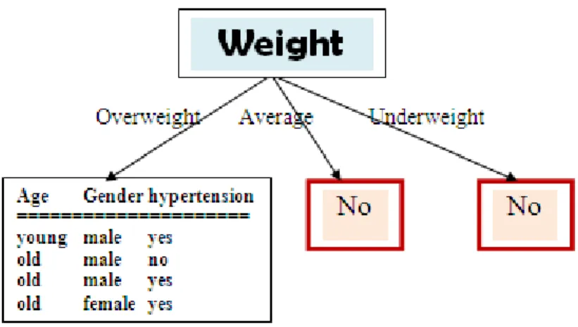
The data in any branch has a homogenous value if the branch has the same value/class for the target attribute. As we can see in the above picture, when
Weight = average, all the data have hypertension = "No", and also when Weight
= underweight, all data values have hypertension = "No" as well. Therefore, these parts of the tree can be represented by leaf nodes. Leaf nodes are nodes with no branches to lower nodes. Consequently, these leaf nodes cannot continue to process the next attribute in a lower branch.
In the next step, having divided the tree by the attribute Weight, we will focus on the branch where Weight = overweight:
Name Age Gender Hypertension
Andy young male yes
Boby old male no
Harley old male yes
The expected information needed to classify a record in the table when
Weight=overweight:
Info(D) = − − = 0.31 +0.50 = 0.81
Using Equation 2.2, the expected information needed to classify a record in D if the records are partitioned according to age attribute is
( ) = ∗ − − 0 + ∗ (− − ) = 0.043
The gain ratio for age attribute would be :
( ) = ( ) − ( ) = 0.81 − 0.043 = 0.767
Similarly, the expected information needed to classify a record in D if the records are partitioned according to gender is :
( ) = ∗ − − + ∗ − − 0 = 0.043
Attribute gender has the same gain ratio as attribute age = 0.767
Therefore, there is no way to determine the next branches except by using expert knowledge or random selection. If we choose Gender to be the next attribute, the tree can be developed as follows:
From the leaf that contains mixed values (yes and no), we can continue the calculation of entropy. Fortunately, age is the last attribute left and we can directly choose the age attribute without calculating the entropy value. The next tree obtained is as follows:
As we can see above, if age=old, there is still a mix of (Yes) and (No) as there is one record with a Yes value and one with a No value. However, we must choose one value; there is no way except using expert knowledge (if available) or using random selection. In Figure 2.1, we choose ‘No’ value if age=old. These illustrations of generating decision trees from the dataset are intended to provide a clear picture about the processes that exist in the decision trees. Besides many other attribute selection measures that have been proposed, we use two methods of attribute selection measures: Chi-Square Automatic Interaction Detector (CHAID) in SPSS and the Classification Regression Trees (CART) in MATLAB. Both methods are used in chapter 3 to develop risk of mortality and in chapter 4 to develop early warning score.
CHAID method was designed in South Africa by (Kass, 1980). This was a decision tree which used a measure based on the statistical chi-test 2).
Breiman et al., (1984) developed a CART algorithm for obtaining the binary decision trees in which every node has two branches. It uses an attribute selection measure called the Gini Index.
The Gini index measures the impurity of D, a data partition or set of training records, as:
Equation 2.4: ( ) = 1 −
Where pi is the probability that a record in D belongs to class Ci and is estimated by , /| |. The sum is computed over m classes.
The Gini index considers a binary split for each attribute. Let’s first consider the case where A is a discrete-valued attribute having v distinct values, [a1, a2, ... ,av] occurring in D.
In case of binary split, there was a computation of all impurity of every division. For instance, if a binary split on A divides D into D1 and D1, the Gini index of D says that the given partition is in equation 2.5.
Equation 2.5: ( ) = | |
| | ( ) +
| |
| | ( )
By the binary split on a discrete-or continuous valued attribute A can lead to lowering in impurity:
Equation 2.6:
2.2.2
Transformation of a decision tree into
decision rules
Decision Trees provide a representation that is intuitive and easily understandable by humans. But to actually generate the ou