Central among the questions explored in biology are those that seek to understand the timing and rates of evolutionary processes. Accurate estimates of species divergence times are vital to understanding historical biogeography, estimating diversification rates, and identifying the causes of variation in rates of molecular evolution.
This tutorial will provide a general overview of divergence time estimation and fossil calibration in a Bayesian framework. The exercise will guide you through the steps necessary for estimating phylogenetic relationships and dating species divergences using the program BEAST v1.7.5.
Background: Divergence time estimation
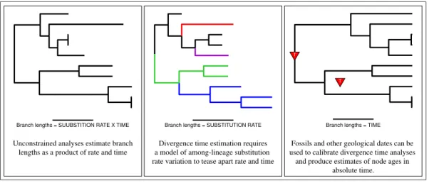
Estimating branch lengths in proportion to time is confounded by the fact that the rate of evolution and time are intrinsically linked when inferring genetic differences between species. A model of lineage-specific substitution rate variation must be applied to tease apart rate and time. When applied in methods for divergence time estimation, the resulting trees have branch lengths that are proportional to time. External node age estimates from the fossil record or other sources are necessary for inferring the real-time (or absolute) ages of lineage divergences (Figure1).
Branch lengths = SUUBSTITION RATE X TIME Unconstrained analyses estimate branch
lengths as a product of rate and time
Branch lengths = SUBSTITUTION RATE Divergence time estimation requires a model of among-lineage substitution rate variation to tease apart rate and time
Branch lengths = TIME Fossils and other geological dates can be used to calibrate divergence time analyses and produce estimates of node ages in
absolute time. T T
Figure 1: Estimating branch lengths in units of time requires a model of lineage-specific rate variation, a model for describing the distribution of speciation events over time, and external information to calibrate the tree.
Ultimately, the goal of Bayesian divergence time estimation is to estimate the joint posterior probability,
P(R,T |S,C), of the branch rates (R) and times (T) given a set of sequences (S) and calibration information (C):
P(R,T | S,C) = P(S | R,T) P(R) P(T | C)
P(S | C) ,
whereP(S|R,T) is the likelihood,P(R) is the prior probability of the rates, P(T |C) is the prior probability of the times, and P(S|C) is the marginal probability of the data. We use numerical methods—Markov chain Monte Carlo (MCMC)—to eliminate the difficult task of calculating the marginal probability of the data. Thus, our primary focus, aside from the tree topology, is devising probability distributions for the prior on the rates, P(R), and the prior on the times, P(T |C).
Modeling lineage-specific substitution rates
Many factors can influence the rate of substitution in a population such as mutation rate, population size, generation time, and selection. As a result, many models have been proposed that describe how substitution rate may vary across the Tree of Life.
The simplest model, the molecular clock, assumes that the rate of substitution remains constant over time
(Zuckerkandl and Pauling, 1962). However, many studies have shown that molecular data (in general)
violate the assumption of a molecular clock and that there exists considerable variation in the rates of substitution among lineages.
Several models have been developed and implemented for inferring divergence times without assuming a strict molecular clock and are commonly applied to empirical data sets. Many of these models have been applied as priors using Bayesian inference methods. The implementation of dating methods in a Bayesian framework provides a flexible way to model rate variation and obtain reliable estimates of speciation times, provided the assumptions of the models are adequate. When coupled with numerical methods, such as MCMC, for approximating the posterior probability distribution of parameters, Bayesian methods are extremely powerful for estimating the parameters of a statistical model and are widely used in phylogenetics.
Some models of lineage-specific rate variation:
• Global molecular clock: a constant rate of substitution over time (Zuckerkandl and Pauling,1962) • Local molecular clocks (Kishino, Miyata and Hasegawa,1990;Rambaut and Bromham, 1998; Yang
and Yoder,2003;Drummond and Suchard,2010)
– Closely related lineages share the same rate and rates are clustered by sub-clades
• Compound Poisson process (Huelsenbeck, Larget and Swofford,2000)
– Rate changes occur along lineages according to a point process and at rate-change events, the new rate is a product of the old rate and a Γ-distributed multiplier.
• Autocorrelated rates: substitution rates evolve gradually over the tree
– Log-normally distributed rates: the rate at a node is drawn from a log-normal distribution with a mean equal to the parent rate (Thorne, Kishino and Painter,1998;Kishino, Thorne and
Bruno,2001;Thorne and Kishino,2002)
– Cox-Ingersoll-Ross Process: the rate of the daughter branch is determined a non-central χ2
distribution. This process includes a parameter that determines the intensity of the force that drives the process to its stationary distribution (Lepage et al.,2006).
• Uncorrelated rates
– The rate associated with each branch is drawn from a single underlying parametric distribution such as an exponential or log-normal (Drummond et al.,2006;Rannala and Yang,2007;Lepage
et al.,2007).
• Infinite mixture model on branch rates
– Branches are assigned to distinct rate categories according to a Dirichlet process (Heath, Holder
and Huelsenbeck,2012).
The variety of models for relaxing the molecular clock assumption presents a challenge for investigators interested in estimating divergence times. Some models assume that rates are heritable and autocorrelated over the tree, others model rate change as a step-wise process, and others assume that the rates on each branch are independently drawn from a single distribution. Furthermore, studies comparing the accuracy (using simulation) or precision of different models have produced conflicting results, some favoring uncorrelated models (Drummond et al.,2006) and others preferring autocorrelated models (Lepage et al.,
2007). Because of this, it is important for researchers performing these analyses to consider and test different relaxed clock models (Lepage et al.,2007;Ronquist et al.,2012;Li and Drummond,2012;?). It is also critical to take into account the scale of the question when estimating divergence times. For example, it might not be reasonable to assume that rates are autocorrelated if the data set includes very distantly related taxa and low taxon sampling. In such cases, it is unlikely that any signal of autocorrelation is detectible.
Priors on node times
There are many component parts that make up a Bayesian analysis of divergence time. One that is often overlooked is the prior on node times, often called a tree prior. This model describes how speciation events are distributed over time. When this model is combined with a model for branch rate, Bayesian inference allows you to estimate relative divergence times. Furthermore, because the rate and time are confounded in the branch-length parameter, the prior describing the branching times can have a strong effect on divergence time estimation.
We can separate the priors on node ages into different categories:
• Phenomenological—models that make no explicit assumptions about the biological processes that
generated the tree. These priors are conditional on the age of the root.
– Uniform distribution: This simple model assumes that internal nodes are uniformly distributed between the root and tip nodes (Lepage et al.,2007; Ronquist et al.,2012).
– Dirichlet distribution: A flat Dirichlet distribution describes the placement of internal nodes on every path between the root and tips (Kishino, Thorne and Bruno,2001;Thorne and Kishino,
2002).
• Mechanistic–models that describe the biological processes responsible for generating the pattern of
lineage divergences.
– Population-level processes—models describing demographic processes (suitable for describing differences among individuals in the same species/population)
∗ Coalescent—These demographic models describe the time, in generations, between
coales-cent events and allow for the estimation of population-level parameters (Kingman,1982a;b;c;
Griffiths and Tavare,1994).
– Species-level processes—stochastic branching models that describe lineage diversification (suit-able for describing the timing of divergences between samples from different species)
∗ Yule (pure-birth) process: The simplest branching model assumes that, at any given point
in time, every living lineage can speciate at the same rate, λ. Because the speciation rate is constant through time, there is an exponential waiting time between speciation eventsYule
(1924); Aldous(2001). The Yule model does not allow for extinction.
∗ Birth-death process: An extension of the Yule process, the birth-death model assumes that
at any point in time every lineage an undergo speciation at rate λ or go extinct at rate µ
(Kendall, 1948; Thompson, 1975; Nee, May and Harvey, 1994; Rannala and Yang, 1996;
Yang and Rannala,1997;Popovic,2004;Aldous and Popovic,2005;Gernhard,2008). Thus,
the Yule process is a special case of the birth-death process where µ= 0.
In BEAST, the available tree priors for divergence time estimation using inter-species sequences are the
the Calibrated Yule, Birth Death Incomplete-Sampling, and Birth-Death Serially Sampled. Other programs also offer speciation priors as well as some alternative priors such as a uniform prior
(PhyloBayes, MrBayes v3.2, DPPDiv), a Dirichlet prior (multidivtime), and a birth-death prior with
species sampling (MCMCTree). Priors based on the coalescent which are intended for population-level analyses or time-stamped virus data are also available in BEAST. The effect of different node-time priors on estimates of divergence times is not well understood and appears to be dataset-dependent (Lepage et al.,
2007). Accordingly, it is important to account for the characteristics of your data when choosing a tree prior. If you know that your sequences are from extant species, each from different genera, then it is unlikely that a coalescent model adequately reflects the processes that generated those sequences. And since you do not have any samples from lineages in the past, then you should not use the serial-sampled birth-death model. Furthermore, if you have prior knowledge that extinction has occurred, then a pure-birth (Yule) prior is not appropriate.
Fossil calibration
Without external information to calibrate the tree, divergence time estimation methods can only reliably provide estimates of relative divergence times and not absolute node ages. In the absence of adequate calibration data, relative divergence times are suitable for analyses of rates of continuous trait evolution or understanding relative rates of diversification. However, for some problems, such as those that seek to uncover correlation between biogeographical events and lineage diversification, an absolute time scale is required. Calibration information can come from a variety of sources including “known” substitution rates (often secondary calibrations estimated from a previous study), dated tip sequences from serially sampled data (typically time-stamped virus data), or geological date estimates (fossils or biogeographical data). Age estimates from fossil organisms are the most common form of divergence time calibration information. These data are used as age constraints on their putative ancestral nodes. There are numerous difficulties with incorporating node age estimates from fossil data including disparity in fossilization and sampling, uncertainty in dating, and correct phylogenetic placement of the fossil. Thus, it is critical that careful attention is paid to the paleontological data included in phylogenetic divergence time analyses. With an accurately dated and identified fossil in hand, further consideration is required to determine how to apply the node-age constraint. If the fossil is truly a descendant of the node it calibrates, then it provides a reliable minimum age bound on the ancestral node time. However, maximum bounds are far more difficult to come by. Bayesian methods provide a way to account for uncertainty in fossil calibrations. Prior distributions reflecting our knowledge (or lack thereof) of the amount of elapsed time from the ancestral node to is calibrating fossil are easily incorporated into these methods.
A nice review paper by Ho and Phillips (2009) outlines a number of different parametric distributions appropriate for use as priors on calibrated nodes. In this exercise we will use the uniform, normal, log-normal, and exponential distributions (Figure2).
Uniform distribution – Typically, you must have both maximum and minimum age bounds when applying
a uniform calibration prior (though some methods are available for applying uniform constraints with soft bounds). The minimum bound is provided by the fossil member of the clade. The maximum bound may come from a bracketing method or other external source. This distribution places equal probability across all ages spanning the interval between the lower and upper bounds.
Normal distribution – The normal distribution is not always appropriate for calibrating a node using fossil
information (though some methods allow for assigning a truncated normal prior density). When applying a biogeographical date (e.g. the Isthmus of Panama) or a secondary calibration (a node age estimate from
Time
Uniform (min, max)
Exponential (λ) Gamma (α, β) Minimum age Log Normal (µ, σ) Normal (µ, σ) (fossil)
Figure 2: Five different parametric distributions that can be applied as priors on the age of a calibrated node. a previous study), the normal distribution can be a useful calibration prior. This distribution is always symmetrical and places the greatest prior weight on the mean (µ). Its scale is determined by the standard deviation parameter (σ).
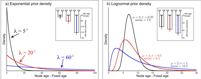
Probability distributions restricted to the interval [0,∞), such as the log-normal, exponential, and gamma are appropriate for use as zero-offset calibration priors. When applying these priors on node age, the fossil age is the origin of the prior distribution. Thus, it is useful to consider the fact that the prior is modeling the amount of time that has elapsed since the divergence event (ancestral node) until the time of the descendant fossil (Figure 3).
λ
= 5
-1λ
= 20
-1λ
= 60
-1 D e n si tyNode age - Fossil age
0 20 40 60 80 100 60 80 100 120 140
a) Exponential prior density
Exp e ct e d n o d e a g e Min age (fossil) Exp e ct e d n o d e a g e Min age (fossil) D e n si ty
Node age - Fossil age
0 5 10 15 20 25 30
30
35
40
45
b) Lognormal prior density
Figure 3: Two common prior densities for calibrating node ages. a) The exponential distribution with three different values for the rate parameter,λ. As the value of theλrate parameter is decreased, the prior becomes less informative (the blue line is the least informative prior, λ = 60−1). The inset shows an example of the three different priors
and their expected values placed on the same node with a minimum age bound of 60. b) The lognormal distribution with 3 different values for the shape parameter,σ. For this distribution, even thoughµis equal to 2.0 for all three, expected value (mean) is dependent on the value ofσ. The inset shows an example of the three different priors and their expected values placed on the same node with a minimum age bound of 30.
Gamma distribution – The gamma distribution is commonly used as a prior on scalar variables in Bayesian inference. It relies on 2 parameters: the scale parameter (α) and a rate parameter (λ). More specifically, the gamma distribution is the sum ofαindependently and identical exponentially distributed random variables with rate λ. Asα becomes very large (α >10), this distribution approaches the normal distribution.
Exponential distribution – The exponential distribution is a special case of the gamma distribution and is
characterized by a single rate parameter (λ) and is useful for calibration if the fossil age is very close to the age of its ancestral node. The expected (mean) age difference under this distribution is equal to λ−1 and
the median is equal to λ−1∗ln(2). Under the exponential distribution, the greatest prior weight is placed
on node ages very close to the age of the fossil with diminishing probability to ∞. Asλis increased, this prior density becomes strongly informative, whereas very low values ofλresult in a fairly non-informative prior (Figure3a).
Log-normal distribution – An offset, log-normal prior on the calibrated node age places the highest
proba-bility on ages somewhat older than the fossil, with non-zero probaproba-bility to∞. If a variable is log-normally distributed with parametersµ and σ, then the natural log of that variable is normally distributed with a mean of µ and standard deviation ofσ. The median of the lognormal distribution is equal to eµ and the mean is equal toeµ+σ
2
2 (Figure 3b).
Programs used in this exercise
BEAST – Bayesian Evolutionary Analysis Sampling Trees
BEAST is a free software package for Bayesian evolutionary analysis of molecular sequences using MCMC and strictly oriented toward inference using rooted, time-measured phylogenetic trees. The development and maintenance of BEAST is a large, collaborative effort and the program includes a wide array of different types of analyses:
• Phylogenetic tree inference under different models for substitution rate variation
– Constant rate molecular clock (Zuckerkandl and Pauling,1962) – Uncorrelated relaxed clocks (Drummond et al.,2006)
– Random local molecular clocks (Drummond and Suchard,2010)
• Estimates of species divergence dates and fossil calibration under a wide range of branch-time models
and calibration methods
• Analysis of non-contemporaneous sequences
• Heterogenous substitution models across data partitions • Population genetic analyses
– Estimation of demographic parameters (population sizes, growth/decline, migration) – Bayesian skyline plots
– Phylogeography (Lemey et al., 2009)
• Gene-tree/species-tree inference (∗BEAST;Heled and Drummond,2010) • and more...
BEAST is written in java and its appearance and functionality are consistent across platforms. Inference using MCMC is done using the BEAST program, however, there are several utility applications that assist in the preparation of input files and summarize output (BEAUti, LogCombiner, and TreeAnnotator are all part of the BEAST software bundle;http://beast.bio.ed.ac.uk).
BEAUti – Bayesian Evolutionary Analysis Utility
BEAUti is a utility program with a graphical user interface for creating BEAST and *BEAST input files which must be written in the eXtensible Markup Language (XML). This application provides a clear way to specify priors, partition data, calibrate internal nodes, etc.
LogCombiner – When multiple (identical) analyses are run using BEAST (or MrBayes), LogCombiner
can be used to combine the parameter log files or tree files into a single file that can then be summarized using Tracer (log files) or TreeAnnotator (tree files). However, it is important to ensure that all analyses reached convergence and sampled the same stationary distribution before combining the parameter files.
TreeAnnotator – TreeAnnotator is used to summarize the posterior sample of trees to produce a
maxi-mum clade credibility tree and summarize the posterior estimates of other parameters that can be easily visualized on the tree (e.g. node height). This program is also useful for comparing a specific tree topology and branching times to the set of trees sampled in the MCMC analysis.
Tracer – Tracer is used for assessing and summarizing the posterior estimates of the various parameters
sampled by the Markov Chain. This program can be used for visual inspection and assessment of conver-gence and it also calculates 95% credible intervals (which approximate the 95% highest posterior density intervals) and effective sample sizes (ESS) of parameters (http://tree.bio.ed.ac.uk/software/tracer).
FigTree – FigTree is an excellent program for viewing trees and producing publication-quality
fig-ures. It can interpret the node-annotations created on the summary trees by TreeAnnotator, allow-ing the user to display node-based statistics (e.g. posterior probabilities) in a visually appealallow-ing way (http://tree.bio.ed.ac.uk/software/figtree).
The eXtensible Markup Language
The eXtensible Markup Language (XML) is a general-purpose markup language, which allows for the combination of text and additional information. In BEAST, the use of the XML makes analysis specification very flexible and readable by both the program and people. The XML file specifies sequences, node calibrations, models, priors, output file names, etc. BEAUti is a useful tool for creating an XML file for many BEAST analyses. However, typically, dataset-specific issues can arise and some understanding of the BEAST-specific XML format is essential for troubleshooting. Additionally, there are a number of interesting models and analyses available in BEAST that cannot be specified using the BEAUti utility program. Refer to the BEAST web page (http://beast.bio.ed.ac.uk/XML format) for detailed information about the BEAST XML format. Box 1 shows an example of BEAST XML syntax for specifying a birth-death prior on node times.
<!-- A prior on the distribution node heights defined given -->
<!-- a Birth-Death speciation process (Gernhard 2008). -->
<birthDeathModel id="birthDeath" units="substitutions"> <birthMinusDeathRate>
<parameter id="birthDeath.meanGrowthRate" value="1.0" lower="0.0" upper="Infinity"/> </birthMinusDeathRate>
<relativeDeathRate>
<parameter id="birthDeath.relativeDeathRate" value="0.5" lower="0.0" upper="Infinity"/> </relativeDeathRate>
</birthDeathModel>
Practical: Divergence time estimation
For this exercise, we will estimate phylogenetic relationships and date the species divergences of the ten simulated sequences in the file called divtime.nex. This simple alignment contains two genes, each 500 nucleotides in length.
• Download all of the compressed directories and place them in a directory you’ve created named: divtime beast. After uncompressing, you should have the files listed in Box 2. (Tutorial url:
http://treethinkers.org/divergence-time-estimation-using-beast/)
• divtime beast/data/
– divtime.nex
– divtime start tree.tre
• divtime beast/output1/ – divtime.log – divtime.prior.log – divtime.trees – divtime.prior.trees – divtime.ops – divtime.prior.ops • divtime beast/output2/ – divtime 100m.1.log – divtime 100m.2.log – divtime 100m.prior.log • divtime beast/output3/ – divtime 100m.1.trees – divtime 100m.2.trees – divtime.comb.trees
Box 2: The data files required for this exercise.
• Open the NEXUS file containing the sequences in your text editor. TheASSUMPTIONSblock contains
the commands for partitioning the alignment into two separate genes (Box 3). Tests for model selection indicated that gene1and gene2evolved under separate GTR+Γ models.
#NEXUS BEGIN DATA;
DIMENSIONS NTAX=10 NCHAR=1000;
FORMAT DATATYPE = DNA GAP = - MISSING = ?; MATRIX T1 CTACGGGAGGGCAACGGGGCTAGATGGTAAACGCGCCATCGATCGCAAG... T2 CTACGGGAGGGCGACGGGGCTAGATGGTAAACGCGCCCTCGATCGCAAG... T3 CAGCGTGAGGGCCACGGGGCTGGCAGGTACTCCGGCCCACGAGTGGAAG... T4 CAGCGTGGGGGCCACGGGGCTAGAAGTTACTCCGGCCCACGAGTGGAAG... T5 CAGCGTGGGGGCCACGGGGCTAGAAGTTACTCCGGCCCACGAGTGGAAG... T6 CAGCGAGAAGCCGACGGGGATGGAAGGGACTCAGACGCACGAGTCCATG... T7 CATCGCGAGGGGGACGGGGCTCGTAGATTATCGTTCATGCAAGCTGAAG... T8 CATCGCGAGGGGGACGGGGCTCGTAGTTTATCGTTCAGGCAAGCTGAAG... T9 CAGCGTGACCACGACGGGGCTGGGGGTGATTCCCGCTGACAAGATGAAG... T10 CTGCGTGACAACGACGGGGCTGGGAGTTGTTCCCGCTCACAAGAGGAAG... ; END; BEGIN ASSUMPTIONS; charset gene1 = 1-500; charset gene2 = 501-1000; END;
Box 3: A fragment of the NEXUS file containing the sequences for this exercise. The data partitions are defined in theASSUMPTIONSblock..
These 10 sequences consist of 6 ingroup taxa: T1, T2, T3, T4, T5, T6 and 4 outgroup taxa: T7, T8, T9, T10. After performing an unconstrained analysis using maximum likelihood, we get the topology in Figure4. The branch lengths estimated under maximum likelihood are indicative of variation in substitu-tion rates. Divergence time estimasubstitu-tion and fossil calibrasubstitu-tion require that you have some prior knowledge of the tree topology so that calibration dates can be properly assigned.
Figure 4: A maximum likelihood estimate of the phylogenetic relationships of divtime.nex. (Constructed using PAUP* v4.0a125;Swofford,1998)
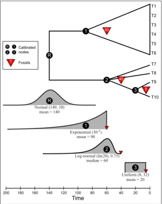
Fossil node calibrations are often difficult to obtain for every node and for many groups they are simply unavailable. In such cases, constraints can be applied to outgroup nodes. There are four calibration points for this data set. These are illustrated in Figure5. The oldest fossil belonging to the ingroup can calibrate the age of that clade. This fossil was identified as a member of the clade, falling within the crown group. Two fossils calibrate nodes within the outgroup clade and a well supported estimate of the root age from a previous study allows us to place a prior distribution on that node (Figure5).
R 1 2 3 Log-normal (ln(20), 0.75) Exponential (30-1) Normal (140, 10) Uniform (8, 32) 3 2 1 R T1 T2 T3 T4 T5 T6 T8 T7 T9 T10 20 40 60 80 100 120 0 160 140 200 180 Time 60 40 8 3 2 1 R Calibrated nodes Fossils T mean = 140 mean = 90 median = 60 mean = 20
Figure 5: Four nodes with fossil calibration for thedivtime.nexdata set. There are calibrations on the root and 3 other internal nodes. Each calibration point is assumed to have a different prior density.
Getting started with BEAUti
Creating a properly-formatted BEAST XML file from scratch is not a simple task. However, BEAUti provides a simple way to navigate the various elements specific to the BEAST XML format.
• Begin by executing the BEAUti program. For Mac OSX and Windows, you can do this by double
clicking on the application. For Unix systems (including Mac OSX), it is convenient to add the entire
BEASTv1.7.5/bindirectory to your path.
• Import the sequences from divtime.nexusing the pull-down menu: File→Import Data.
This example data set contains 2 different partitions labeled gene1 and gene2. When the NEXUS file is imported into BEAUti, the Partitions tab lists each partition and their currently assumed substitution model, clock model, and tree.
• Double click on the file name (divtime.nex) next to one of the data partitions. This will bring up
a window allowing you to visually inspect your alignment.
We would like to analyze each gene under separate substitution models, while assuming the clock and tree are linked.
• Select bothgene1andgene2. While both partitions are highlighted click theUnlink Subst. Models
button. You will notice that the site model listed for gene2has changed. [Figure 6]
Figure 6: Unlink the substitution models for the two data partitions.
• For the sake of clarity, let’s rename theClock Model and Partition Tree. While both partitions
are highlighted, click theLink Clock Models button. This will bring up a window where you can rename the clock model. Check the box next toRename clock model partition to: and provide a new name. The example below calls itdivtimeClock. [Figure7]
Figure 7: Rename the clock model.
• Similarly, rename thePartition Treeby clicking theLink Treesbutton. Perhaps call itdivtimeTree.
Now your Partitions tab should show that the two genes are assumed to have separate substitution models, a single clock model called divtimeClock, and a single tree calleddivtimeTree. [Figure 8] Now that you have set up your data partitions, you can move on to specifying ancestral nodes in the tree for calibration.
Figure 8: The data partitions with unlinked substitution models and linked clock model and tree.
• Go to the Taxa tab.
The options in theTaxa window allow the user to identify internal nodes of interest. Simply creating a taxon set does not necessarily force the clade to be monophyletic nor does it require you to specify a time calibration for that node. Once a taxon set is created, statistics associated with the most recent common ancestor (MRCA) of those taxa (e.g. node height) will be reported in the BEAST parameter log file. For this data set, we will apply external time calibrations to 4 internal nodes (Figure 5), including the root. Because the root node is implicit, we only have to specify 3 internal nodes in theTaxa window.
• Create a new taxon set for calibration node 1 by clicking the + button in the lower, left corner of
the window. Double click on the default name (untitled1) for the taxon set and rename itmrca1. These taxa form our “ingroup” clade, so check the box under the Monophyletic? column. There is also a check-box in the column labeled Stem? this allows the user to specify a calibration for the stem of a clade, thus placing an age constraint on the ancestral node of the MRCA defined by this taxon set. Leave this unchecked since we are assuming that the fossil calibration formrca1is within the crown group. You will also see a text-entry box where you can provide a starting age for the node. This is a new feature of BEAUti 1.7.5 that allows you to use a randomly-generated starting tree that is consistent with your calibrations. We will specify our own starting tree, so leave this box empty. [Figure9]
• In the center panel of the Taxa window, select the taxa descended from calibration node 1 (T1, T2, T3, T4, T5, T6). When you have highlighted each of these taxon names, move them from the
Excluded Taxa column to theIncluded Taxa column by clicking the button with the green arrow.
[Figure9]
Figure 9: Defining the taxon set for the most recent common ancestor of T1, T2, T3, T4, T5, and T6.
• Create a new taxon set for calibration node 2 (T7, T8, T9, T10; Figure 5) and rename itmrca2.
These taxa make up the “outgroup” and should also be monophyletic.
• Make a new taxon set for calibration node 3 called mrca3 (T9, T10; Figure 5). You can leave the
Monophyletic? box unchecked for this set of taxa.
The Tips menu contains the options necessary for analyses of data sets containing non-contemporaneous tips. This is primarily for serial sampled virus data and not applicable to this exercise.
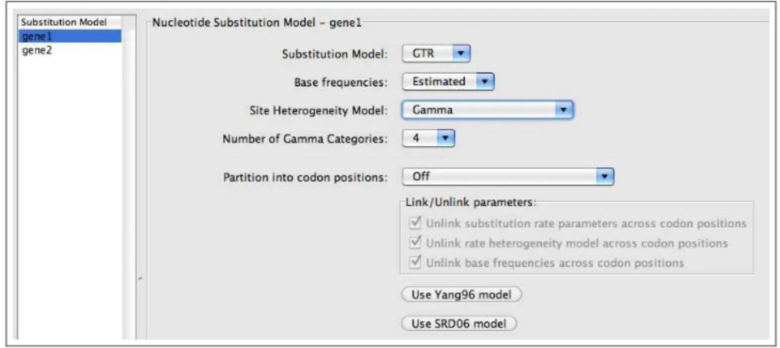
• Go to the Sites menu to specify a substitution model for each of our data partitions. Change the
substitution model for gene1 to GTR, with Estimated base frequencies, and set the among-site heterogeneity model toGamma. [Figure 10]
• Specify a GTR+Γ model forgene2 as well. [Figure10]
Figure 10: Defining a GTR+Γ model forgene1.
You will notice other options in the Sites menu which are specifically for protein-coding data, allowing you to partition your data set by codon position. If you select the button labeled Use Yang96 model, this will specify a codon model for which each of the 3 positions evolves under a different GTR+Γ model (Yang, 1996). The button labeled Use SRD06 Model will set the model parameters to those used in a paper by Shapiro, Rambaut and Drummond(2006) which partitions the data so that 3rd codon positions are analyzed separately from 1st and 2nd positions and assumes a HKY+Γ model. The sequences in this analysis are not protein-coding, so these options are not applicable to this exercise.
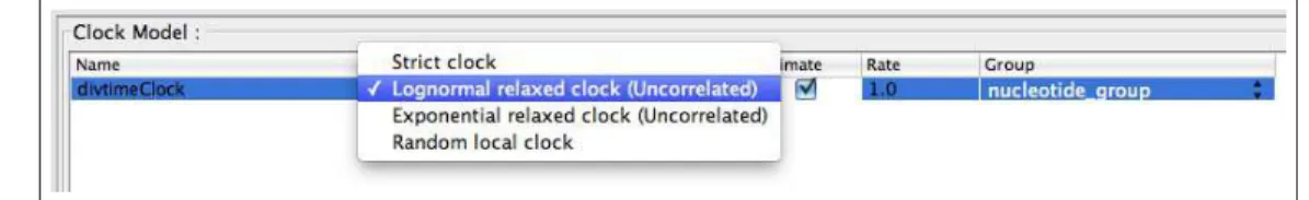
• Move on to the Clocks menu to set up the relaxed clock analysis.
Here, we can specify the model of lineage-specific substitution rate variation. The default model in BEAUti is the Strict Clock with a fixed substitution rate equal to 1. Three models for relaxing the assumption of a constant substitution rate can be specified in BEAUti as well. The Lognormal relaxed clock
(Uncorrelated)option assumes that the substitution rates associated with each branch are independently
drawn from a single, discretized lognormal distribution (Drummond et al.,2006). Under theExponential
relaxed clock (Uncorrelated)model, the rates associated with each branch are exponentially distributed
(Drummond et al.,2006). TheRandom local clock uses Bayesian stochastic search variable selection to
average over random local molecular clocks (Drummond and Suchard,2010).
• Set theClock Model fordivtimeClockto Lognormal relaxed clock (Uncorrelated) and check
the box in the Estimate column. [Figure 11]
Below the settings for the Clock Model there is a box labeled Clock Model Group. The clock group table is used to specify shared molecular clocks, and to set apart clocks applied to different types of data.
• Move on to the Trees window.
In theTreesmenu, you can specify a starting tree and theTree Priorwhich is the prior on the distribution of node times.
Figure 11: Options for modeling among-lineage substitution rate variation in the Clock Model menu.
• Go to the Tree Prior pull-down menu and choose Speciation: Birth-Death Process. [Figure
12]
Figure 12: Setting the birth-death prior distribution on branching times.
This model and those labeled Speciation are appropriate for analyses of inter-species relationships. The
Speciationmodels are stochastic branching processes with a constant rate of speciation (λ) and a constant
rate of extinction (µ). In the case of the Yule model, the extinction rate is equal to 0. Notice that for each of the different tree priors, the relevant citation is provided for you. Both the Yule and birth-death models are implemented in BEAST followingGernhard(2008) with hyper-prior distributions on the parameters of the model. Thus, for the birth-death model used in this analysis, our runs will sample the net diversification rate (meanGrowthRate=λ−µ) and the relative rate of extinction (relativeDeathRate= µλ).
You will notice several other options for the Tree prior available in BEAUti. These priors are differen-tiated by the labels Coalescent,Speciation, or Epidemiology. Coalescent tree priors are appropriate for population-level analyses. Conversely, when you are estimating relationships and divergence times of interspecies data, it is best to employ a speciation prior. Choosing a coalescent prior for estimating deep divergences, or a speciation prior for intra-species data, can often lead to problematic results due to inter-actions between the prior on the node ages and the prior on the branch rates. Thus, it is critical that these priors are chosen judiciously. Furthermore, it is important to note that our understanding of the statistical properties of speciation prior densities combined with calibration densities is somewhat incomplete, par-ticularly when the tree topology is considered a random variable (Heled and Drummond,2012;Warnock,
Yang and Donoghue,2012). The optionSpeciation: Calibrated Yule is a more statistically sound tree
prior when applying a single calibration density. Refer to Heled and Drummond(2012) for more details about this issue.
BEAST also has a few options for initialization of the tree topology and branch lengths. Starting trees can be generated either randomly (under a coalescent model) or with UPGMA. Alternatively, the user can specify the tree by including atreesblock in the NEXUS data file, importing it directly into BEAUti, or by pasting the Newick string and XML elements in the XML file.
We would like to use our own starting tree. The starting tree topology can come from any type of analysis. For this data set, we performed an initial analysis using maximum likelihood resulting in the tree in Figure 4. Using the maximum likelihood tree topology, branch lengths were generated by drawing them from a uniform distribution conditional on the node age constraints from the fossil record. For this exercise, the file called divtime start tree.treis a NEXUS formatted file containing the starting tree. [Figure 13]
R
1
2
3
Figure 13: Starting tree. The topology was inferred using maximum likelihood and the node heights were drawn from a uniform distribution with constraints on the root and 3 internal nodes.
• Load the starting tree using the pull-down menu: File→Import Data. Import the NEXUS file
containing your starting tree: divtime start tree.tre(you may have to change theFile Format
to All Files). This will jump you back to the Partitions window.
• Return to theTrees window and select User-specified starting tree in theTree Model section.
Next to the option Select-user specified tree: choose ml tre. [Figure 14]
Figure 14: Specifying a starting tree.
The States panel allows one to specify analyses for ancestral state reconstruction and provides sequence
error model options for any data partition. Leave these options unmodified.
• Navigate to the Priors menu.
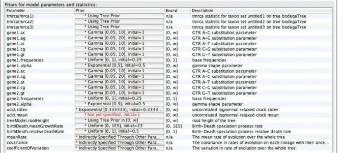
In the Priors window, all of the model parameters and statistics specified in earlier menus are listed. Here you can set prior distributions on substitution model parameters, calibration nodes, and parameters associated with the clock model and tree model. [Figure15]
The prior on the ucld.meanparameter is indicated in red because it is not set by default in this version of BEAUti. When you click on the box for this prior you will see a window allowing you to specify a prior distribution on the mean rate of substitution. In Bayesian terminology this parameter is ahyperparameter
because it is a parameter describing a prior distribution and not a direct parameter of the data model (like base frequencies or branch lengths). In Bayesian inference a prior distribution can be placed on a hyperparameter, and this is called ahyperprior. By allowing the value of this hyperparameter to vary, we are freed from the responsibility of fixing the mean of the log-normal prior distribution on branch-specific substitution rates. Additionally, the Markov chain will sample this hyperparameter along with the other
Figure 15: The statistics, parameters, and hyperparameters specific to this analysis and default priors. parameters directly associated with the models on our data, providing us with an estimate of the posterior distribution.
• Click on the prior for ucld.meanand specify anExponential distribution on this hyperparameter
with a mean equal to 10.0. [Figure 16]
Figure 16: Exponential prior distribution on theucld.meanhyperparameter.
Review the hyperparameters of the birth-death model. For this model the average net diversification rate is meanGrowthRate = λ−µ and the relative rate of extinction is relativeDeathRate= µλ. Under the birth-death model implemented in BEAST, the net diversification rate (meanGrowthRate) must be greater than zero (µ < λ). Therefore, the relative death rate can only take on values between 0 and 1. The default priors for these parameters are both uniform distributions.
Next, we can specify prior distributions on calibrated node ages. Each of the 4 calibrated nodes (Figure 5) requires a different type of prior distribution on their respective ages. Notice that the current prior for each of our calibrated nodes is set to: Using Tree Prior. If we did not have constraints on the ages of the clades defined in the Taxa menu, the times for these divergences will be sampled, just like all the others, with the prior being the birth-death model. By creating thesetmrcaparameters in the Taxa window, we have created a statistic that will be logged to our output file.
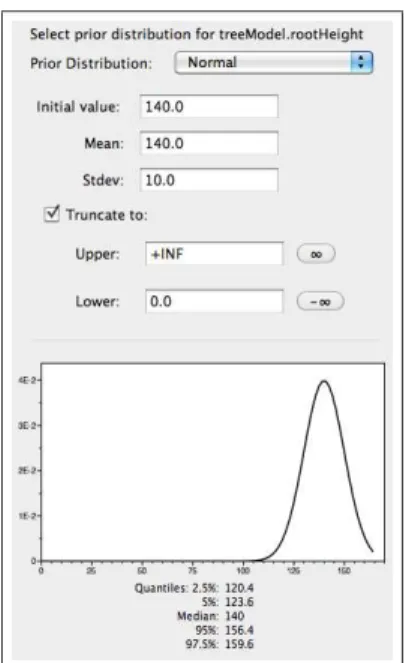
• Set a normal distribution on the age of the root. Click on the prior box for thetreeModel.rootHeight
parameter and chooseNormal. Parameterize the normal distribution so that theMeanandInitial
Value are equal to140and theStdev (standard deviation) is equal to10. For this prior, the value
is truncated so that the age of the root cannot be less than 0. Leave the box indicating a truncated normal distribution checked. The normal distribution is not always appropriate for representing fossil age constraints, but is useful for imposing a prior requiring soft minimum and maximum bounds. Typically, this type of prior on the calibrated node age is based on biogeographical data or when a secondary calibration date is used. [Figure 17]
Figure 17: A normal prior distribution on the age of the root.
A fossil age constraint is available for the most recent common ancestor of our ingroup, mrca1 (T1, T2, T3, T4, T5, T6). This minimum age estimate will serve as a hard lower bound on the age that node. Thus, the prior distribution on this node will be offset by the age of the fossil (60). When applying off-set priors on nodes, it is perhaps easiest to consider the fact that the distribution is modeling the time difference between the age of the calibrated node and the age of the fossil (see Figure3). We are applying an exponential prior on the age of mrca1. The exponential distribution is characterized by a single rate parameter (λ), which controls both the mean and variance. The expected (mean) age difference under this distribution is equal toλ−1 and the median is equal toλ−1∗ln(2). Specifying the exponential prior on a
node age in BEAST requires that you set theexpected age difference between the node and fossil (Mean) and the hard lower bound (Offset).
• Click on the prior box next to tmrca(mrca1)and set the prior distribution on the age of mrca1to
an Exponential with a Mean equal to 30 and Offset equal to 60. The quantiles for this prior
probability will be below 170.67 My. [Figure18] 0 60 0.03 0.01 0.02 160 140 120 100 80 D e n si ty
Node Age (My) Quantiles 2.5%: 5%: Median (50%): 95%: 97.5%: 60.76 61.54 80.79 149.87 170.67 Offset Exponential Prior Density for tmrca(mrca1)
Figure 18: An offset exponential prior on the calibration nodemrca1.
The fossil calibration for the MRCA of the outgroup (T7, T8, T9, T10) provides a minimum age bound for the age of mrca2. The log-normal distribution is often used to describe the age of an ancestral node in relation to a fossil descendant. If a random variable, χ, is log-normally distributed with parameters µ
and σ: χ∼LN(µ, σ), then the natural log of that variable is normally distributed with a mean of µ and standard deviation of σ: log(χ) ∼ Norm(µ, σ). The median of the lognormal distribution is equal to eµ
and the mean (or expectation) is:
E(χ) =eµ+
σ2 2 .
When applying the lognormal offset prior distribution on node age in BEAST, first consider the expected age difference between the MRCA and the fossil. Generally, it is difficult to know with any certainty the time lag between the speciation event and the appearance of the fossil and, typically, we prefer to specify prior densities that are not overly informative (Heath,2012).
For the prior density onmrca2, we will specify a lognormal prior density with an expected value equal to 20. Thus, if we want the expectation of the lognormal distribution to equal 20, we must determine the value forµ using the equation above solve forµ:
µ = ln(20)−0.75 2
2 = 2.714482,
where 0.75 is the standard deviation parameter of the lognormal distribution for this particular fossil calibration.
• Select the prior box next to tmrca(mrca2)and specify a Lognormal prior distribution for mrca2
and setLog(Mean) to µ= 2.714482. The age of the fossil is40 time units; use this date to set the
Offset for the lognormal prior distribution. Finally, set theLog(Stdev) to 0.75, so that 97.5% of
the prior probability is below 105.7. [Figure 19A]
Notice that the window for theLognormal prior distribution allows you to specifyMean in Real Space. If you choose this option, then the mean value you enter is the expected value of the lognormal distribution. You will specify the exact same distribution as above if you set theLog(Mean) to 20while this option is selected. [Figure19B]
A B
Figure 19: A log-normal prior distribution to calibratemrca2. A) Specifying theLog(Mean). B) SelectingMean in Real Space. A bug in BEAUti v1.7.0 causes the plot of the prior density to disappear when you specify an
Offset value.
It is important that you are very careful when specifying these parameters. If, for example,Mean in Real
Space was checked and you provided a value of 2.714482for theLog(Mean), then your calibration prior
density would be very informative. In the case of the prior ontmrca(mrca2), this would place 95% of the prior density below 47.03566. Conversely, if you set the Log(Mean) to 20, your calibration prior would be extremely diffuse, with a median value of 485,165,235!
The node leading to taxa T9 and T10 will be calibrated using a simple uniform distribution. For this calibration we will be placing a hard minimum and a hard maximum bound on the age of mrca3. Fossil data typically provide us with reliable minimum constraints on the age of a clade. And although absolute maximum bounds are very difficult to obtain, uniform priors with hard lower and upper age constraints are often used for divergence time estimation. Some methods using phylogenetic bracketing and stratigraphic bounding have been developed for determining possible maximum bounds (Marshall, 1990; 1994; 1997;
Benton and Donoghue,2007;Marshall,2008), though it is best to apply soft age maxima when using these
methods.
• Select the prior box next to tmrca(mrca3)and set the Uniform prior distribution on the time of mrca3with a Lower limit of 8and an Upper limit of 32. [Figure 20]
Figure 20: A uniform prior distribution on the age of mrca3with hard lower and upper bounds.
TheOperatorsmenu contains a list of the parameters and hyperparameters that will be sampled over the course of the MCMC run. In this window, it is possible to turn off any of the elements listed to fix a given parameter to its starting value. For example, if you would like to estimate divergence times on a fixed tree topology (using a starting tree that you provided), then disable proposals operating on theTree. For this exercise, leave this window unmodified.
Now that you have specified all of your data elements, models, priors, and operators, go to the MCMC
tab to set the length of the Markov chain, sample frequency, and file names. By default, BEAST sets the number of generations to 10,000,000.
• Since we have a limited amount of time for this exercise, change theLength of chain to 1,000,000.
(Runtimes may vary depending on your computer, if you have reason to believe that this may take a very long time, then change the run length to something smaller.)
The frequency parameters are sampled and logged to file can be altered in the box labeledLog parameters
every. In general, this value should be set relative to the length of the chain to avoid generating excessively
large output files. If a low value is specified, the output files containing the parameter values and trees will be very large, possibly without gaining much additional information. Conversely, if you specify an exceedingly large sample interval, then you will not get enough information about the posterior distributions of your parameters.
• ChangeLog parameters every to 100.
• The frequency states are echoed to the screen is simply for observing the progress of your run, so set
this to a satisfactory value (such as1000), keeping in mind that writing to the screen too frequently can cause the program to run slower. Specify the output file name prefix divtime in File name
stem.
Now you are ready to generate your BEAST XML file!
• Click on the button in the lower right corner: Generate BEAST File...
You will see a window that will allow you to see the priors that you have not reviewed. This window also warns you about improper priors.
• It is safe to proceed, so click Continue and save your XML file with the name divtime.xml.
For the last step in BEAUti, generate an XML file that will run the analysis on an “empty” dataset and sample only from the prior. This allows us to evaluate the priors we have applied to the various parameters and hyperparameters in our analysis. BEAUti creates this file by simply replacing the nucleotide sequences in the XML file with a series of missing states: NNNN. Running this file in BEAST will produce output files that we can use to visualize the priors and compare them to our posterior estimates.
• Check the box next to Sample from prior only - create empty alignment. Be sure to change
theFile name stem to divtime.prior and the XML file name todivtime.prior.xmlafter you
click Generate BEAST File... , so that you do not over-write your analysis files. Then close
Making changes in the XML file
BEAUti is a great tool for generating a properly-formatted XML file for many types of BEAST analyses. However, you may encounter errors that require modifying elements in your input file and if you wish to make small to moderate changes to your analysis, altering the input file is far less tedious than generating a new one using BEAUti. Furthermore, BEAST is a rich program and all of the types of analyses, models, and parameters available in the core cannot be specified using BEAUti. Thus, some understanding of the BEAST XML format is essential.
If you attempted to execute divtime.xml in BEAST right now, the analysis would terminate due to an error resulting from issues with the specification of the truncated normal prior on the root height in BEAUti. For other datasets, you may run into problems if you use a randomly-generated starting tree that is not compatible with calibrations on nodes.
• Open thedivtime.xml file generated by BEAUti in your text editor and glance over the contents.
BEAUti provides many comments describing each of the elements in the file.
As you look over the contents of this file, you will notice that the components are specified in an order similar to the steps you took in BEAUti. The XML syntax is very verbose. This feature makes it fairly easy to understand the different elements of the BEAST input file. If you wished to alter your analysis or realized that you misspecified a prior parameter, changing the XML file is far simpler than going through all of the steps in BEAUti again. For example, if you wanted to change bounds of the uniform prior on
mrca3 from (8, 32) to (12, 30), this can be done easily by altering these values in the XML file (Box 4), though leave these at 8 and 32 for this exercise.
<uniformPrior lower="8.0" upper="32.0"> <statistic idref="tmrca(mrca3)"> </uniformPrior>
Box 4: The XML syntax for specifying a uniform prior distribution on tmrca(mrca3). Changing the parameters (highlighted) of this prior is simply done by altering the XML file.
For our analysis, there is one setting causes an error when this XML file is executed in BEAST (Box 5). This is a problem with the truncated prior on the age of the root node.
Error parsing ‘<uniformPrior>’ element with id, ‘null’:
Uniform prior uniformPrior cannot take a bound at infinity, because it returns 1/(high-low) = 1/inf
Box 5: BEAST error from truncated normal prior.
• We can easily correct this problem if we edit the XML file. Find the priors specified for the parameter
calledtreeModel.rootHeightin your XML file. These priors are specified in the section delineated by the comment: Define MCMC(Box 6). Use the find function in your text editor to find this problem.
<uniformPrior lower="0.0" upper="Infinity"> <parameter idref="treeModel.rootHeight"> </uniformPrior>
<normalPrior mean="140.0" stdev="10.0"> <parameter idref="treeModel.rootHeight"> </normalPrior>
Box 6: The truncated normal prior distribution on thetreeModel.rootHeight. The error results from the upper bound on theuniformPrior.
• Because the improper uniform prior doesn’t integrate to 1.0, BEAST returns an error. This can
be fixed by either giving the uniformPrioran upper bound equal to some arbitrarily chosen, high value (change Infinity to 100000.0) or by deleting the syntax describing the uniformPrior on
treeModel.rootHeight altogether (delete everything highlighted in yellow in Box 6). Since the height of the root node is always bounded by the ages of its descendant nodes, the age is already truncated (Box 6).
• Make these changes for both of the XML files created in BEAUti (divtime.xmlanddivtime.prior.xml).
Look over the elements specified in each of the XML files and verify that everything is satisfactory. Save and close the input files.
Although running multiple, independent analyses is an important part of any Bayesian analysis, BEAST does not do this by default. However, setting up multiple runs is trivial once you have a complete XML file in hand and only requires that you make a copy of the input file and alter the names of the output files in the XML (it’s also best to change the initial states for all of your parameters, including the starting tree).
Running BEAST
Now you are ready to start your BEAST analysis. BEAST allows you to use the BEAGLE library if you already have it installed. BEAGLE is an application programming interface and library that effectively takes advantage of your computer hardware (CPUs and GPUs) for doing the heavy lifting (likelihood calculation) needed for statistical phylogenetic inference (Ayers et al., 2012). Particularly, when using BEAGLE’s GPU (NVIDIA) implementation, runtimes are significantly shorter.
• Execute divtime.prior.xmland divtime.xmlin BEAST. You should see the screen output every
1,000 generations, reporting the likelihood and several other statistics.
• Once you have verified that your XML file was properly configured and you see the likelihood update,
feel free to kill the run. I have provided the output files for this analysis and you can find them in
divtime beast/output*.
Summarizing the output
Once the run reaches the end of the chain, you will find three new files in your analysis directory. The MCMC samples of various scalar parameters and statistics are written to the file called divtime.log. The tree-state at every sampled iteration is saved to divtime.trees. The tree strings in this file are all annotated in extended Newick format with the substitution rate from the uncorrelated lognormal model at each node. The files called divtime.opsand mcmc.operators(these files may be identical) summarize the performance of each of the proposal mechanisms (operators) used in your analysis. Reviewing this file can help identify operators that might need adjustment if their acceptance probabilities are too high. The main output files are the .logfile and .treesfile. It is not feasible to review the data contained in these files by simply opening them in a spreadsheet program or a tree viewing program. Fortunately, the developers of BEAST have also written general utility programs for summarizing and visualizing posterior samples from Bayesian inference using MCMC. Tracer is a cross-platform, java program for summarizing posterior samples of scaler parameters. This program is necessary for assessing convergence, mixing, and determining an adequate burn-in. Tree topologies, branch rates, and node heights are summarized using the program TreeAnnotator and visualized in FigTree.
Tracer
This section will briefly cover using Tracer and visual inspection of the analysis output for MCMC conver-gence diagnostics.
• Open Tracer and import the divtime.logfile in the File→Import New Trace File.
You will notice, in the Estimates tab, that many items in the ESS column are red. The MCMC runs you have performed today are all far too short to produce adequate posterior estimates of divergence times and substitution model parameters and this is reflected in the ESS values. The ESS is theeffective sample size of a parameter. The value indicates the number of effectively independent draws from the posterior in the sample. This statistic can help to identify autocorrelation in your samples that might result from poor mixing. It is important that you run your chains long enough and sufficiently sample the stationary distribution so that the ESS values of your parameters are all high (over 200 or so).
• Click on a parameter with a low ESS and explore the various windows in Tracer. It is clear that we
must run the MCMC chain longer to get good estimates.
Provided with the files for this exercise are the output files from analyses run for 100,000,000 iterations. These files can be found in thedivtime beast/output2/directory and are all labeled with the file stem:
divtime 100m*.
• Closedivtime.login Tracer using the - button and opendivtime 100m.1.log,divtime 100m.2.log
and divtime 100m.prior.log.
These log files are from much longer runs and since we ran two independent, identical analyses, we can compare the log files in Tracer and determine if they have converged on the same stationary distribution. Additionally, analyzing an empty alignment allows you to compare your posterior estimates to the prior distributions used for each parameter.
• Select and highlight all three files (divtime 100m.1.log,divtime 100m.2.logand
divtime 100m.prior.log) in the Trace Files pane (do not include Combined). This allows you to compare all three runs simultaneously. Click on the various parameters and view how they differ in their estimates and 95% credible intervals for those parameters.
The 95% credible interval is a Bayesian measure of uncertainty that accounts for the data. If we use the 95% credible interval, this means that the probability the true value of a parameter lies within this interval is 0.95, given our model and data. This measure is often used to approximate the 95% highest posterior density region (HPD).
• Find the parameter ucld.stdevand compare the estimates of the standard deviation of the
uncor-related log-normal distribution.
Theucld.stdevindicates the amount of variation in the substitution rates across branches. Our prior on this parameter is an exponential distribution withλ= 3.0 (mean= 0.33333). Thus, there is a considerable amount of prior weight on ucld.stdev = 0. A standard deviation of 0 indicates support for no variation in substitution rates and the presence of a molecular clock.
• Withucld.stdevhighlighted for all three runs, go to theMarginal Density window, which allows
Figure 21: Comparing the marginal densities of theucld.stdevparameter from 2 independent runs (red and gray) and the prior (blue) in Tracer.
• Color (or “colour”) the densities byTrace File next toColour by at the bottom of the window (if
you do not see this option, increase the size of your Tracer window). You can also add aLegend to reveal which density belongs to which run file. [Figure21]
The first thing you will notice from this plot is that the marginal densities from each of our analysis runs (divtime 100m.1.logand divtime 100m.2.log) are nearly identical. If you click through the other sampled parameters, these densities are the same for each one. This indicates that both of our runs have converged on the same stationary distribution. Since some of the other parameters might not have mixed well, we may want to run them longer, but we can have good confidence that our runs have sampled the same distribution.
Second, notice how the marginal densities for the ucld.stdev parameter from each of the analysis runs are quite different from the marginal density of that parameter sampled from the prior. The signal in the data is not overwhelmed by the prior on this parameter. Moreover, our analysis runs do not have any significant density at zero, indicating no support for a constant rate of substitution (e.g. strict molecular clock). This is also evident if you view the 95% credible intervals (95% HPD) for each of the runs. When the analyses are run with data, aucld.stdev of 0 does not fall within the credible interval.
When calibrating divergence time estimates using off-set parametric prior densities, it is very important to evaluate (and report) the marginal densities of both the prior and posterior samples of calibrated node heights.
• Highlight only the trace file containing MCMC samples under the prior (divtime 100m.prior.log).
Then inspect the Marginal Density for each one. The prior densities are quite close to the cali-bration priors we specified in BEAUti and described in Figure5.
• Specifically, look at the marginal prior density of tmrca(mrca1). The calibration prior assigned to
this node was an exponential density with a rate (orλ) equal to 1
30. We expect the marginal density of the age of that node sampled under the prior to match the expected prior density. In Figure22, you can see that the marginal prior density of the age of mrca1 (purple line) closely fits an exponential distribution with a rate equal to 1
0 0.005 0.01 0.015 0.02 0.025 0.03 0.035 0.04 60 80 100 120 140 160 180 Density
Node Age (mrca1)
true age
Marginal posterior density (observed)
Marginal prior density (observed)
Exponential(1/30) density (expected)
Figure 22: Comparing the marginal density oftmrca(mrca1)(purple line) to the exponential prior density specified for that calibration node (black line). (This figure was generated usinggnuplotand can also be made inR.) Because the two analysis runs (divtime 100m.1.logand divtime 100m.2.log) sampled from the same posterior distribution, particularly for the parameters we are interested in, they can be combined. Tracer does this when you import files and you will see a file called Combined in theTrace Files window. To use this option, however, you must first remove the prior trace file.
• Highlight only the prior file (divtime 100m.prior.log) in the Trace Files pane. Click the
-button below the window to remove the file.
• Now highlight the Combined trace file. Navigate through the sampled parameters and notice how
the ESSs have improved.
Continue examining the options in Tracer. This program is very useful for exploring many aspects of your analysis.
Summarizing the trees
After reviewing the trace files from the two independent runs in Tracer and verifying that both runs converged on the posterior distributions and reached stationarity, we can combine the sampled trees into a single tree file and summarize the results.
• Open the program LogCombiner and set theFile type to Tree Files. Next, import the twotrees
files in thedivtime beast/output3/directory (divtime 100m.1.treesanddivtime 100m.2.trees) using the + button. [Figure23]
These analyses were each run for 100,000,000 iterations with a sample frequency of 10,000. Therefore, each of the trees files contains 100,000 trees.
• Set a burn-in value of 2,500, thus discarding the first 25% of the samples in each tree file. Then click
on the Choose file ... button to create an output file (call it divtime.comb.trees) and run the program. [Figure23]
• Alternatively, use LogCombiner in unix with the command:
Figure 23: Use LogCombiner to combine the trees from two independent, identical runs.
Once LogCombiner has terminated, you will have a file containing 10,000 trees calleddivtime.comb.trees
which can be summarized using TreeAnnotator. TreeAnnotator takes a collection of trees and summarizes them by identifying the topology with the best support, calculating clade posterior probabilities, and calculating 95% credible intervals for node-specific parameters. All of the node statistics are annotated on the tree topology for each node in the Newick string.
• Open the program TreeAnnotator. Since we already discarded a set of burn-in trees when combining
the tree files, we can leave Burnin set to0. [Figure24]
Figure 24: Set up tree summary in TreeAnnotator.
• For theTarget tree type, choose Maximum clade credibility tree.
TheMaximum clade credibility tree is the topology with the highest product of clade posterior
prob-abilities across all nodes. Alternatively, you can select theMaximum sum of clade credibilities which sums all of the clade posteriors. Or you can provide a target tree from file.
ThePosterior probability limitoption applies to summaries on a target tree topology and only calculates
posteriors for nodes that are above the specified limit.
• Choose Median heights or Mean heights for Node heights which will set the node heights of
the output tree to equal the median or mean height for each node in the sample of trees.
• Choosedivtime.comb.treesas yourInput Tree File. Then name theOutput File: divtime.fig.tre
and click Run. [Figure24]
Once the program has finished running, you will find the filedivtime.fig.trein your directory.
• Open divtime.fig.tre in your text editor. The tree is written in NEXUS format. Look at the
tree string and notice the annotation. Each node in the tree is labeled with comments using the
An alternative program to LogCombiner and TreeAnnotator isSumTrees, a program in the DendroPy package (Sukumaran and Holder,2010). SumTrees is very flexible and allows more options than TreeAn-notator and it provides a way to summarize sets of trees from a number of different programs and analyses. The tree summaries produced by TreeAnnotator or SumTrees can be opened with FigTree. FigTree reads the comments for each each node and can display them in a variety of ways.
• Open FigTree and open the filedivtime.fig.tre.
FigTree is a great tree-viewing program and it also allows you to produce publication-quality tree figures. This summary tree is shown in Figure25. The posterior probabilities are labeled on each branch (they are almost all equal to 1). The branches of the tree are colored by the average substitution rate estimated for each lineage. On each node, bars are displayed representing the node age 95% credible interval.
Figure 25: The final tree with node bars representing the age 95% credible intervals and posterior probabilities of each clade labeled on the branches. Each branch is colored according to the average substitution rate sampled by the MCMC chain.
• Explore the various options for creating a tree figure and recreate the tree in Figure 25. The figure
you create can be exported as a PDF or EPS file.
Divergence time estimation for this simulated data set is very straight-forward. To generate the sequences for this exercise I first simulated a tree topology and divergence times under a constant-rate birth-death process with 10 extant taxa (T1, T2, T3, T4, T5, T6, T7, T8, T9, T10). The simulated time-tree is shown in Figure26A.
With a tree topology and branch lengths in units of time, I simulated lineage-specific substitution rate variation under an uncorrelated model such that the rate associated with each branch was drawn from a log-normal distribution (Figure26B). The tree with branch lengths in units ofrate∗timewas then used to simulate two separate genes each under a different GTR+Γ model. For the most part, the models assumed in this analysis matched the models used to generate the data, therefore our estimates of divergence time and tree topology are quite accurate. We inferred the correct tree topology and the true divergence times all fall within the node age 95% credible intervals.
Time substitutions/site
A B
Figure 26: A) The true tree and branching times. The age of the root is equal to 147.28. B) The true tree and branch lengths in units ofrate∗time. The branches are colored according to their substitution rate.
Useful Links
• BEAST website and documentation: http://beast.bio.ed.ac.uk • BEAST open source project: http://code.google.com/p/beast-mcmc
• Join the BEAST user discussion: http://groups.google.com/group/beast-users
• BEAST2 (under development, a complete rewrite of BEAST1): http://beast2.cs.auckland.ac.nz • MrBayes: http://mrbayes.sourceforge.net/
• DPPDiv: http://phylo.bio.ku.edu/content/tracy-heath-dppdiv • PhyloBayes: www.phylobayes.org/
• multidivtime: http://statgen.ncsu.edu/thorne/multidivtime.html • MCMCtree (PAML):http://abacus.gene.ucl.ac.uk/software/paml.html • BEAGLE: http://code.google.com/p/beagle-lib/
• A list of programs: http://evolution.genetics.washington.edu/phylip/software.html#Stratigraphy • The Paleobiology Database: http://www.paleodb.org
• The Fossil Record & Date A Clade: http://www.fossilrecord.net
Questions about this tutorial can be directed to Tracy Heath (email: [email protected]).
Relevant References
Aldous D. 2001. Stochastic models and descriptive statistics for phylogenetic trees, from yule to today. Statistical Science. 16:23–34.
Aldous D, Popovic L. 2005. A critical branching process model for biodiversity. Advances in Applied Probability. 37:1094–1115.
Aris-Brosou S, Yang Z. 2002. Effects of models of rate evolution on estimation of divergence dates with special reference to the metazoan 18s ribosomal rna phylogeny. Systematic Biology. 51:703–714.
Aris-Brosou S, Yang Z. 2003. Bayesian models of episodic evolution support a late precambrian explosive diversification of the metazoa. Molecular Biology and Evolution. 20:1947–54.
Ayers DL, Darling A, Zwickl DJ, et al. (12 co-authors). 2012. BEAGLE: An application programming interface and high-performance computing library for statistical phylogenetics. Systematic Biology. 61:170–173.
Baele G, Lemey P, Bedford T, Rambaut A, Suchard MA, Alekseyenko AV. 2012. Improving the accuracy of demographic and molecular clock model comparison while accommodating phylogenetic uncertainty. Molecular Biology and Evolution. 30:2157–2167.
Baele G, Li WLS, Drummond AJ, Suchard MA, Lemey P. 2013. Accurate model selection of relaxed molecular clocks in Bayesian phylogenetics. Molecular Biology and Evolution. 30:239–243.
Benton MJ, Ayala FJ. 2003. Dating the tree of life. Science. 300:1698–1700.
Benton MJ, Donoghue PCJ. 2007. Paleontological evidence to date the tree of life. Molecular Biology and Evolution. 24:26–53.
Benton MJ, Wills MA, Hitchin R. 2000. Quality of the fossil record through time. Nature. 403:534–537. Brown R, Yang Z. 2011. Rate variation and estimation of divergence times using strict and relaxed clocks.
BMC Evolutionary Biology. 11:271.
Cutler DJ. 2000a. Estimating divergence times in the presence of an overdispersed molecular clock. Molec-ular Biology and Evolution. 17:1647–1660.
Cutler DJ. 2000b. Understanding the overdispersed molecular clock. Genetics. 154:1403–1417.
Darriba D, Aberer A, Flouri T, Heath T, Izquierdo-Carrasco F, Stamatakis A. 2013. Boosting the per-formance of Bayesian divergence time estimation with the phylogenetic likelihood library. 12th IEEE International Workshop on High Performance Computational Biology. .
dos Reis M, Inoue J, Hasegawa M, Asher R, Donoghue P, Yang Z. 2012. Phylogenomic datasets provide both precision and accuracy in estimating the timescale of placental mammal phylogeny. Proceedings of the Royal Society B: Biological Sciences. 279:3491–3500.
dos Reis M, Yang Z. 2011. Approximate likelihood calculation on a phylogeny for bayesian estimation of divergence times. Molecular Biology and Evolution. 28:2161–2172.
dos Reis M, Yang Z. 2012. The unbearable uncertainty of Bayesian divergence time estimation. Journal of Systematics and Evolution. 51:30–43.
Doyle JA, Donoghue MJ. 1993. Phylogenies and angiosperm diversification. Paleobiology. 19:141–167. Drummond A, Pybus O, Rambaut A, Forsberg R, Rodrigo A. 2003. Measurably evolving populations.
Trends in Ecology & Evolution. 18:481–488.
Drummond AJ, Ho SY, Phillips MJ, Rambaut A. 2006. Relaxed phylogenetics and dating with confidence. PLoS Biology. 4:e88.
Drummond AJ, Rambaut A. 2007. BEAST: Bayesian evolutionary analysis by sampling trees. BMC Evolutionary Biology. 7:214.