Distributed Estimation and Inference for the Analysis of Big Biomedical Data

Distributed Estimation and Inference for the

Analysis of Big Biomedical Data

by

Emily C. Hector

A dissertation submitted in partial fulfillment of the requirements for the degree of

Doctor of Philosophy (Biostatistics)

in The University of Michigan 2020

Doctoral Committee:

Professor Peter X.-K. Song, Chair

Professor Veerabhadran Baladandayuthapani Professor Xuming He

Emily C. Hector [email protected]

ORCID iD: 0000-0003-1488-3150

ACKNOWLEDGEMENTS

It is a challenge to know where to begin. During my graduate studies in the Department of Biostatistics at the University of Michigan I have had the great privilege of working with generous, passionate, kind and brilliant colleagues and friends, without whom the journey and its final product would have been impossible. I will try to do them justice.

I am grateful to my parents and sister for their love, encouragement and support. They lead by example, living with balance, purpose, empathy and curiosity. I strive to be better because of them.

To my many friends and colleagues, especially Andrew Whiteman, thank you for your love, support and friendship. There have been times of challenge and of great happiness, and every moment was enriched by your presence. In alphabetical order, particular thanks go to Margaret Banker, Marco Benedetti, Mathieu Bray, Wei Hao, Holly Hartman, Lan Luo, Adam Peterson, Kelly Speth, Lu Tang, Lili Wang, Lu Xia, Xianyong Yin, Ling Zhou and Yiwang Zhou. I would also like to thank the Biostatistics department staff, and especially Nicole Fenech, for their tireless work. I extend my sincere thanks to my many collaborators in the ELEMENT team, including Jackie Goodrich, Erica Jansen, Karen Peterson and Wei Perng, and to Tianwei Yu and Laura Scott, for their collaboration and guidance. I am grateful to Markku Laakso for generously letting me use his data in my third project. Special thanks go to Michael Boehnke for his generosity, support and accumen, and to the

chair of the Biostatistics department, Bhramar Mukherjee, for her time, counsel and example. They foster a rich, diverse and stimulating environment in our department, and it is difficult to imagine Michigan without them.

I am deeply indebted to my committee for their time, advice and contributions, and especially: to Xuming He for his encouragement to do difficult theory that led to a new and deeper understanding and great improvement of my work; to Veera Baladandayuthapani for his insights, wisdom and kindness.

I am extremely grateful to Jian Kang, a mentor, motivator and supporter, for his invaluable encouragement and guidance over the past six years that have greatly enriched my graduate experience. I count myself lucky to have him as a mentor. Thank you for your brilliance.

Most of all, I cannot begin to express my deepest gratitude to my advisor, mentor and friend, Peter Song. I admire his approach of looking for elegant solutions to complex problems. His mentorship has put me on the path to becoming the statistician I aspire to be, and his deep insights have helped me hone my intuition. His enthusiasm and passion for research and data are infectious. He does so much for his students and I want to thank him for that. I hope to someday inspire my students the way he has inspired me.

TABLE OF CONTENTS

DEDICATION . . . ii

ACKNOWLEDGEMENTS. . . iii

LIST OF TABLES . . . vii

LIST OF FIGURES . . . viii

LIST OF APPENDICES . . . xi

ABSTRACT. . . xii

CHAPTER I. Introduction . . . 1

1.1 Motivation . . . 1

1.2 Big Data Challenges . . . 2

1.2.1 Modelling Challenges . . . 2

1.2.2 Computational Challenges . . . 3

1.2.3 Theoretical Challenges . . . 3

1.3 Objectives . . . 4

II. Modelling Correlated Data: a Framework . . . 7

2.1 Introduction . . . 7

2.2 Estimation . . . 9

2.2.1 Joint Modelling Approaches . . . 9

2.2.2 Likelihood-Derived Approaches . . . 10

2.2.3 Estimating Equation Approaches . . . 12

2.3 A Unifying Framework: Estimating Function Theory . . . 14

III. A Distributed and Integrated Method of Moments for High-Dimensional Correlated Data Analysis . . . 19

3.1 Introduction . . . 19

3.2 Formulation . . . 25

3.2.1 Division: Distributed Composite Likelihoods . . . 26

3.2.2 Integration: the Generalized Method of Moments . . . 29

3.3 Asymptotic Properties . . . 32

3.4 Implementation: the Parallelized One-Step Estimator . . . 36

3.5 Simulations . . . 39

3.6 Application to Infant EEG Data . . . 45

IV. Doubly Distributed Supervised Learning and Inference with

High-Dimensional Correlated Outcomes . . . 52

4.1 Introduction . . . 52

4.2 Formulation . . . 56

4.2.1 Double Data Split Procedure . . . 57

4.2.2 Integration . . . 60

4.3 Examples . . . 63

4.3.1 Likelihood-based methods . . . 63

4.3.2 Generalized estimating equations . . . 64

4.3.3 M-estimation . . . 65

4.3.4 Joint mean-variance modelling . . . 65

4.3.5 Marginal quantile regression for correlated data . . . 66

4.4 Asymptotic Properties . . . 67

4.5 Distributed Estimation and Inference . . . 72

4.5.1 Construction ofĈk,i . . . 73

4.5.2 Asymptotic results forK andJ fixed . . . 74

4.5.3 Asymptotic results for divergingKwithJ fixed . . . 77

4.5.4 Asymptotic results for divergingKandJ . . . 80

4.6 Simulations . . . 83

4.7 Discussion . . . 86

V. Joint Integrative Analysis of Multiple Data Sources with Correlated Vector Outcomes . . . 88

5.1 Introduction . . . 88

5.2 Distributed and integrated quadratic inference functions . . . 91

5.2.1 Model formulation . . . 91

5.2.2 Quadratic Inference Functions . . . 93

5.2.3 Integrated Estimator . . . 94

5.2.4 Large sample theory . . . 97

5.3 Simulations . . . 99

5.4 Real Data Analysis . . . 103

5.5 Discussion . . . 106

VI. Summary and Future Work. . . 108

APPENDICES . . . .114

LIST OF TABLES

Table

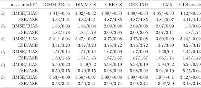
3.1 Simulation results: RMSE, BIAS, ESE, ASE with five covariates,N =1,000,M =

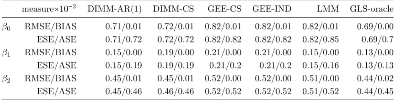
200,J=5, averaged over 500 simulations. . . 41 3.2 Simulation results: RMSE, BIAS, ESE, ASE with two covariates,N =1,000,M =

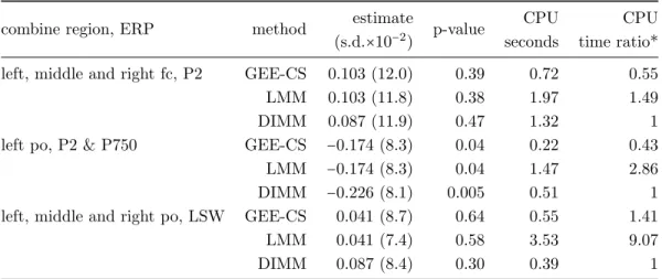
1,000,J=5, averaged over 500 simulations. . . 42 3.3 Select EEG data analysis results: iron sufficiency status effect estimates and

statistics for each combination scheme. . . 47 4.1 Double division of outcome data on both the dimension of responses (into blocks)

and sample size (into groups). . . 55 4.2 Mean CPU time in seconds for each setting with the GEE block analysis, averaged

over 1,000 simulations. Mean CPU time is computed as the maximum CPU time taken over parallelized block analyses added to the CPU time taken by the rest of the procedure. . . 85 4.3 RMSE×10−3_{, BIAS}×₁₀−4_{, ESE}×₁₀−3_{, ASE}×₁₀−3_{for each setting and each covariate,}

averaged over 500 simulations. . . 86 5.1 Logistic regression simulation results with homogeneity partition P = {(j, k)}J,K_j,k=1

(G=1,d1=J K). . . 101 5.2 Logistic regression simulation results with P = {P1,P2,P3},

P1 = {(1, k),(2, k)}K k=1, P2 = {(3, k)} K k=1 and P3 = {(4, k),(5, k)} K k=1, and exchangeable working block correlation structure. . . 102 5.3 Linear regression simulation results with homogeneity partition P = {(j, k)}J,K_j,k=1

(G=1,d1=J K). . . 103 5.4 Metabolite data structure schematic. . . 104 6.1 Comparison of advantages and limitations of methods proposed in Chapters III, IV

and V. . . 112 D.1 Iron sufficiency status effect mean squared error (MSE×10−2_{) and mean variance}

(mean var×10−2_{), 95% confidence interval (CI) coverage, type-1 error, and mean}

CPU time in seconds for each combination scheme based on 500 simulations. . . 140 D.2 Block specific MCLE’s ofβ. . . 141 D.3 Iron sufficiency status effect estimates and statistics for each combination scheme. . 142 E.1 Summary of sensitivity formulas. Formulas that are not used are marked “—”.

*“w.r.t.” shorthand for “with respect to”. . . 143 I.1 Logistic regression simulation setting two results withP = {P1,P2,P3}and AR(1)

working block correlation structure. . . 157 I.2 Dictionary for the short-hand names of the sub-pathways. . . 160 I.3 Estimated effects of smoking for the heterogeneous model. Starred sub-pathways

have a significant effect of smoking at level 0.05/8. s.e. standard error. . . 187 I.4 Estimated effects of smoking for the integrative model. Sub-pathways separated by

a semi-colon have been combined in the integrative analysis. Starred sub-pathway combinations have a significant effect of smoking at level 0.05/8. s.e. standard error. 190

LIST OF FIGURES

Figure

2.1 Schematic of general procedure. . . 18 3.1 (a) Average P2 amplitude for iron sufficient children under stimulus of mother’s

voice. Color plot and additional plots in Appendix D. (b) Layout of the 64 channel sensor net with brain regions related to auditory recognition memory. . . 23 3.2 Plot of electrical potential for subject 1 at electrode 2 over time. . . 24 3.3 Upper panels: comparison of computation time on log10scale of five methods for varying

dimension M based on 500 simulations. Lower panels: comparison of 95% confidence interval coverage of four methods for varying dimensionM based on 500 simulations. Left column hasX1∼ N (0,1); middle column hasX1∼ NM(0, S), whereSis a positive-definite M×M matrix, andX2 a vector of alternating 0’s and 1’s; right column hasX1∼ N (0,1), X2 ∼ Bernoulli(0.3), X3 ∼ M ultinomial(0.1,0.2,0.4,0.25,0.05), X4 ∼ U nif orm(0,1),

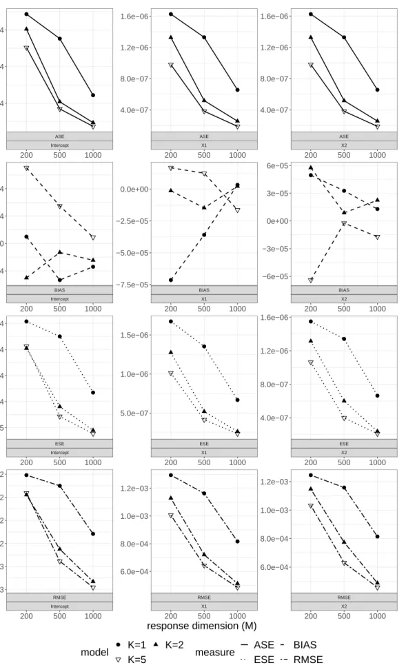
andX5an interaction betweenX1 andX2. . . 44 3.4 RMSE, BIAS, ESE, ASE based on 100 simulations with an intercept and five covariates,

andM=10,000. Covariates are simulated as in the right column of Figure 3.3. . . 44

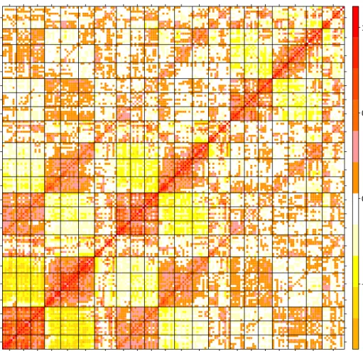
3.5 Correlation of electrical amplitude at three ERP’s for iron sufficient children under stimulus of mother’s voice (color plot and additional plots in Appendix D). . . 45 4.1 Plot of simulation metrics for GEE, averaged over 1,000 simulations. . . 84 C.1 Comparison of type-1 error rate for three methods for varying dimensionM based

on 500 simulations. Left column has X1 ∼ N (0,1); middle column has

X1∼ NM(0, S), where S is a positive-definite M×M matrix, andX2 a vector of alternating 0’s and 1’s; right column has X1 ∼ N (0,1), X2 ∼ Bernoulli(0.3),

X3 ∼ M ultinomial(0.1,0.2,0.4,0.25,0.05), X4 ∼ U nif orm(0,1), and X5 an interaction betweenX1andX2. . . 127 C.2 Chi-squared Q-Q plot of goodness-of-fit test statistics with theoretical 95%

confidence bands based on 500 simulations with one covariate X1 ∼ N (0,1),

M =200,J =3, under correct and incorrect covariance structure specification. . . 128 C.3 Chi-squared Q-Q plot of goodness-of-fit test statistics with theoretical 95%

confidence bands based on 500 simulations with one covariate X1 ∼ N (0,1),

M =200,J =5, under correct and incorrect covariance structure specification. . . 129 C.4 Chi-squared Q-Q plot of goodness-of-fit test statistics with theoretical 95%

confidence bands based on 500 simulations with two covariates

X1 ∼ N ormalM(0, S), where S is a positive-definite M ×M matrix, and X2 a vector of alternating 0’s and 1’s to imitate an exposure, M = 200, J = 3, under correct and incorrect covariance structure specification. . . 130 C.5 Chi-squared Q-Q plot of goodness-of-fit test statistics with theoretical 95%

confidence bands based on 500 simulations with two covariates

X1 ∼ N ormalM(0, S), where S is a positive-definite M ×M matrix, and X2 a vector of alternating 0’s and 1’s to imitate an exposure, M = 200, J = 5, under correct and incorrect covariance structure specification. . . 131 D.1 Average P2 amplitude for iron sufficient and deficient children (left and right panels

respectively) under stimulus of mother and stranger’s voice (top and bottom panels respectively). . . 133

D.2 Average P750 amplitude for iron sufficient and deficient children (left and right panels respectively) under stimulus of mother and stranger’s voice (top and bottom panels respectively). . . 134 D.3 Average LSW amplitude for iron sufficient and deficient children (left and right panels

respectively) under stimulus of mother and stranger’s voice (top and bottom panels respectively). . . 135 D.4 Correlation of electrical amplitude at three ERP’s for iron sufficient children under

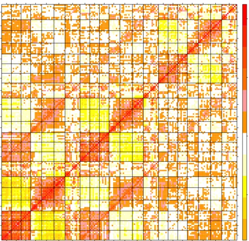
stimulus of mother’s voice. . . 136 D.5 Correlation of electrical amplitude at three ERP’s for iron sufficient children under

stimulus of stranger’s voice. . . 137 D.6 Correlation of electrical amplitude at three ERP’s for iron deficient children under stimulus

of mother’s voice. . . 138 D.7 Correlation of electrical amplitude at three ERP’s for iron deficient children under stimulus

of stranger’s voice. . . 139 G.1 Plot of simulation metrics for CL, averaged over 1,000 simulations. . . 154 I.1 Chi-squared quantile-quantile plot of test statistics in Theorem 2 with theoretical

95% confidence bands based on 500 simulations under correct and incorrect working block covariance structure. The simulation set-up is that of the second set of simulations (J=5,P = {Pg}3g=1). . . 159 I.2 Estimated regression parameters for the amino acid pathway from the

heterogeneous model. . . 163 I.3 Estimated regression parameters for the carbohydrate pathway from the

heterogeneous model. . . 164 I.4 Estimated regression parameters for the cofactors and vitamins pathway from the

heterogeneous model. . . 165 I.5 Estimated regression parameters for the energy pathway from the heterogeneous

model. . . 166 I.6 Estimated regression parameters for the lipid pathway from the heterogeneous

model. . . 167 I.7 Estimated regression parameters for the nucleotide pathway from the heterogeneous

model. . . 168 I.8 Estimated regression parameters for the peptide pathway from the heterogeneous

model. . . 169 I.9 Estimated regression parameters for the xenobiotics pathway from the

heterogeneous model. . . 170 I.10 Estimated regression parameters for the amino acid pathway from the integrative

model. . . 171 I.11 Estimated regression parameters for the carbohydrate pathway from the integrative

model. . . 172 I.12 Estimated regression parameters for the cofactors and vitamins pathway from the

integrative model. . . 173 I.13 Estimated regression parameters for the energy pathway from the integrative model. 174 I.14 Estimated regression parameters for the lipid pathway from the integrative model. 175 I.15 Estimated regression parameters for the nucleotide pathway from the integrative

model. . . 176 I.16 Estimated regression parameters for the peptide pathway from the integrative

model. . . 177 I.17 Estimated regression parameters for the xenobiotics pathway from the integrative

model. . . 178 I.18 Estimated smoking effect for the amino acid pathway from the heterogeneous and

integrative models categorized by significance at the 0.05/8 level. . . 179 I.19 Estimated smoking effect for the carbohydrate pathway from the heterogeneous

I.20 Estimated smoking effect for the cofactors and vitamins pathway from the heterogeneous and integrative models categorized by significance at the 0.05/8 level. . . 181 I.21 Estimated smoking effect for the energy pathway from the heterogeneous and

integrative models categorized by significance at the 0.05/8 level. . . 182 I.22 Estimated smoking effect for the lipid pathway from the heterogeneous and

integrative models categorized by significance at the 0.05/8 level. . . 183 I.23 Estimated smoking effect for the nucleotide pathway from the heterogeneous and

integrative models categorized by significance at the 0.05/8 level. . . 184 I.24 Estimated smoking effect for the peptide pathway from the heterogeneous and

integrative models categorized by significance at the 0.05/8 level. . . 185 I.25 Estimated smoking effect for the xenobiotics pathway from the heterogeneous and

LIST OF APPENDICES

Appendix

A. Chapter III: Proofs . . . 115

B. Chapter III: Regularization of Weight Matrix . . . 125

C. Chapter III: Additional Simulation Results . . . 127

D. Chapter III: Additional Data Analysis Results . . . 132

E. Chapter IV: Technical Details . . . 143

F. Chapter IV: Proofs . . . 145

G. Chapter IV: Additional Simulation Results . . . 153

H. Chapter V: Proofs . . . 155

ABSTRACT

This thesis focuses on developing and implementing new statistical methods to address some of the current difficulties encountered in the analysis of high-dimensional correlated biomedical data. Following the divide-and-conquer paradigm, I develop a theoretically sound and computationally tractable class of distributed statistical methods that are made accessible to practitioners through R statistical software.

This thesis aims to establish a class of distributed statistical methods for regression analyses with very large outcome variables arising in many biomedical fields, such as in metabolomic or imaging research. The general distributed procedure divides data into blocks that are analyzed on a parallelized computational platform and combines these separate results via Hansen’s (1982) generalized method of moments. These new methods provide distributed and efficient statistical inference in many different regression settings. Computational efficiency is achieved by leveraging recent developments in large scale computing, such as the MapReduce paradigm on the Hadoop platform.

In the first project presented in Chapter III, I develop a divide-and-conquer procedure implemented in a parallelized computational scheme for statistical estimation and inference of regression parameters with high-dimensional correlated responses. This project is motivated by an electroencephalography study whose goal is to determine the effect of iron deficiency on infant auditory recognition

memory. The proposed method (published as Hector and Song (2020a)), the Distributed and Integrated Method of Moments (DIMM), divides responses into subvectors to be analyzed in parallel using pairwise composite likelihood, and combines results using an optimal one-step meta-estimator.

In the second project presented in Chapter IV, I develop an extended theoretical framework of distributed estimation and inference to incorporate a broad range of classical statistical models and biomedical data types. To reduce computational speed and meet data privacy demands, I propose to divide data by outcomes and subjects, leading to a doubly divide-and-conquer paradigm. I also address parameter heterogeneity explicitly for added flexibility. I establish a new theoretical framework for the analysis of a broad class of big data problems to facilitate valid statistical inference for biomedical researchers. Possible applications include genomic data, metabolomic data, longitudinal and spatial data, and many more. In the third project presented in Chapter V, I propose a distributed quadratic inference function framework to jointly estimate regression parameters from multiple potentially heterogeneous data sources with correlated vector outcomes. This project is motivated by the analysis of the association between smoking and metabolites in a large cohort study. The primary goal of this joint integrative analysis is to estimate covariate effects on all outcomes through a marginal regression model in a statistically and computationally efficient way. To overcome computational and modeling challenges arising from the high-dimensional likelihood of the correlated vector outcomes, I propose to analyze each data source using Qu et al.’s quadratic inference funtions, and then to jointly reestimate parameters from each data source by accounting for correlation between data sources.

CHAPTER I

Introduction

1.1 Motivation

Recent technological and computational advances have greatly reduced the cost of data generation and storage, leading to a new era of “big data”: data that is massive in volume, velocity, variety and complexity (Secchi, 2018). The wealth of information available presents an opportunity to gain unique insights in biomedical research. In particular, these developments have paved the way for new, exciting and meaningful scientific research in fields such as neuroscience, genomics, personalized medicine, and many more. Statisticians and applied researchers tend to formulate a hypothesis about the data generated by a scientific study and test its validity, with accompanying measures of uncertainty, to gain insights into the data. Several difficulties arise when applying this approach to high-dimensional data. With increasingly complex data, it becomes increasingly difficult to ask the right questions of the data, and obtain a meaningful and nuanced answer. Moreover, high dimensionality can lead to incorrect statistical inference and scientific conclusions due to noise accumulation, spurious correlations, and incidental endogeneity (Fan et al., 2014). Finally, classical statistical methods are burdened with tremendous, and oftentimes prohibitive computational costs when

applied to high-dimensional datasets.

In this dissertation, I focus on developing divide-and-conquer solutions to the problem of analyzing high-dimensional response vectors with complex correlation structure. I describe the key computational and statistical challenges posed by this problem below.

1.2 Big Data Challenges

1.2.1 Modelling Challenges

When Big Data consists of a large number of correlated random variables, as is frequently the case for example in brain imaging, modelling their joint distribution can be challenging for many reasons. It can be difficult to model the full distribution of the data or high-order moments, especially as the number of moments increases beyond the sample size, because of a lack of information on them. Additionally, it can be challenging to capture the variety and heterogeneity of the data without using a large number of parameters, or to determine homogeneity/heterogeneity of these parameters. To address some of these difficulties, Qu et al. (2000) propose the Quadratic Inference Function (QIF) for generalized linear models with correlated outcomes. While this function does not model the correlation parameters, it imposes a correlation structure on the entire high-dimensional correlation structure, which can be statistically inefficient. In practice, when dealing with complex multi-level dependent data, it is ideal to begin by modelling local correlation structures and aggregate them into a global correlation specification. Indeed it is relatively easy to use a simple correlation structure, such as compound symmetry or AR(1), to appropriately capture local correlation. I will propose methods to estimate and carry out inference in a computationally efficient distributed fashion for a set of parameters of interest without modelling higher-order moments. The flexibility of

these methods allows the high-dimensional response to have a complex multi-level correlation structure, minimizing loss of statistical efficiency.

1.2.2 Computational Challenges

One of the key computational challenges with correlated big data stem from inverting large matrices and optimizing over a large number of parameters (Cressie and Johannesson, 2008; Banerjee et al., 2008). Furthermore, iterative algorithms need to repeatedly evaluate an objective function over a very large dataset, which can be time consuming. Modern computing platforms use distributed systems to store data on different servers, and recent computing and algorithmic advances allow statistical methods to be run in a distributed fashion when the data on different servers are independent; computing platforms include the MapReduce paradigm on the Hadoop platform (Khezr and Navimipour, 2017) and Apache Spark (Zaharia et al., 2010); recent algorithmic advances include kernel ridge regression (Zhang et al., 2015b) and matrix factorization (Mackey et al., 2015). It is unclear how to proceed, however, when data on different servers are dependent. Moreover, these platforms are not accessible to applied researchers working in the biomedical field, who tend to work with R or SAS. Finally, some of these platforms, such as Apache Spark, still have an iterative component to them that is computationally challenging. I will provide distributed estimation and inference solutions for correlated distributed data problems that are of interest to applied researchers, with an R package for ease of implementation.

1.2.3 Theoretical Challenges

Theoretical challenges related to a large number of covariates p with a small sample size n are discussed in Johnstone and Titterington (2009). More frequently,

biomedical big data includes a large number of observations on a large number of subjects. These massive datasets are often created by combining various datasets from different sources, such as multi-center cohort studies or consortia, which can lead to data heterogeneity and modelling challenges, as discussed above. More importantly, this data aggregation relies on a crucial independence assumption that is often not met. While the literature on combining information from independent sources is extensive (Singh et al., 2005; Xie et al., 2011; Lin and Xi, 2011; Xie and Singh, 2013; Chen and Xie, 2014; Claggett et al., 2014; Yang et al., 2014a; Battey et al., 2015; Liu et al., 2015; Tang and Song, 2016), to my knowledge no method has been proposed to combine information from dependent sources that provides a thorough description of the accompanying theory. In this dissertation, I establish needed methodology and asymptotic results for combining information from dependent sources.

1.3 Objectives

In this thesis, I focus on developing and implementing new statistical methods to address some of the current difficulties encountered in the analysis of high-dimensional correlated biomedical data. Following the divide-and-conquer paradigm, I develop a theoretically sound and computationally tractable class of distributed statistical methods that are made accessible to practitioners through R statistical software.

This thesis aims to establish a class of distributed statistical methods for regression analyses with very large outcome variables arising in many biomedical fields, such as in genetic or imaging research. The general distributed procedure divides data into blocks that are analyzed on a parallelized computational platform and

combines these separate results via Hansen (1982)’s generalized method of moments. These new methods provide distributed and efficient statistical inference in many different regression settings. Computational efficiency is achieved by leveraging recent developments in large scale computing, such as the MapReduce paradigm on the Hadoop platform.

In Chapter III, I aim to address the modelling, computational, and theoretical challenges related to estimation and inference for regression parameters with high-dimensional responses with multi-level nested correlation structure. This project is motivated by an electroencephalography study whose goal is to determine the effect of iron deficiency on infant auditory recognition memory. I develop the Distributed and Integrated Method of Moments (DIMM) (Hector and Song, 2020a), a divide-and-conquer procedure implemented in a parallelized computational scheme. The DIMM divides responses into subvectors to be analyzed in parallel using pairwise composite likelihood, and combines results using an optimal one-step meta-estimator.

In Chapter IV, I aim to generalize the DIMM to types of analyses other than regression, and to further reduce the computational burden associated with high-dimensional correlated data. I also aim to establishing a clear theoretical foundation for this generalized DIMM. I develop an extended theoretical framework of distributed estimation and inference to incorporate a broad range of classical statistical models and biomedical data types. To reduce computational speed and meet data privacy demands, I propose to divide data by outcomes and subjects, leading to a doubly divide-and-conquer paradigm. I also address parameter heterogeneity explicitly for added flexibility. I establish a new theoretical framework for the analysis of a broad class of big data problems to facilitate valid

statistical inference for biomedical researchers. Possible applications include genomic data, metabolomic data, longitudinal and spatial data, and many more. In Chapter V, I propose a distributed quadratic inference function framework to jointly estimate regression parameters from multiple potentially heterogeneous data sources with correlated vector outcomes. This project is motivated by the analysis of the association between smoking and metabolites in a large cohort study. The primary goal of this joint integrative analysis is to estimate covariate effects on all outcomes through a marginal regression model in a statistically and computationally efficient way. To overcome computational and modeling challenges arising from the high-dimensional likelihood of the correlated vector outcomes, I propose to analyze each data source using Qu et al. (2000)’s QIF, and then to jointly reestimate parameters from each data source by accounting for correlation between data sources.

CHAPTER II

Modelling Correlated Data: a Framework

2.1 Introduction

The first part of this chapter is devoted to describing general approaches to modelling correlated data, and the second part to the general framework proposed in this thesis. I consider inference for an M-dimensional vector of correlated responses y_i with associated covariate Xi, for i=1, . . . , N. Denote

y_i = ( _y

i1 . . . yiM ) T

, Xi= ( _x

i1 . . . xiM ).

Covariates xij, j =1, . . . , M, are q-dimensional column vectors and may include an intercept. In a parametric or semi-parametric framework, the goal is to efficiently estimate and carry out inference for a parameter of interest θ, where y_i are independent realizations of Yi which depend onθ through their distribution:

Yi∣X_i ind.∼ f(y∣X =X_i;θ,Γ_i), i=1, . . . , N.

Γi represents other parameters required for the specification of the distribution of

y_i. Denote by Θ the parameter space of θ. Two main models are of interest and detailed below:

to the dispersion model family of distributions (Jørgensen, 1987):

f(yij;µij, σ_ij2) =a(yij;σ_ij2)exp{− 1 2σ2

ij

d(yij;µij)}, j=1, . . . , M,

with mean µij and dispersion σ2

ij. d(y, µ) is the deviance function, and a(y;σ2)

is a normalizing term. Given a known link function h, the mean and dispersion parameters can be modelled as

h(µij) =η(x_ij;β), log(σ_ij2) =ξ(x_ij;ζ) j=1, . . . , M,

where η and ξ are systematic components. The parameter of interest θ may be any subset of(β,ζ). θmay take several forms such as a vector of regression coefficients in the Generalized Linear Model (GLM), a set of nonparametric regression functions as in the Generalized Additive Model (GAM), a nonparametric function and a vector of regression coefficients as in the semi-parametric model, and many more. See Chapter 4 of Song (2007) for a thorough discussion.

(b) (Marginal Quantile Regression) Quantile regression (Koenker and Bassett, 1978) models the quantiles of the response, rather than the mean, as a function of covariates. It provides a more comprehensive description of the relationship between response and covariates because it has ability to model any point in the distribution. To model the marginal quantiles of y_i, following Lu and Fan (2015) let the τth _{quantile of y}

ij given xij be

Qτ(y_ij∣x_ij) =xT_ijθ_τ. (2.1)

In median regression, the parameter of interest becomesθ=θ₂ (where the 2 indicates the 2-quantile). Quantile regression also has the advantage of not specifying the error distribution, contrary to GLM. Thus, marginal quantile regression is useful when distributional assumptions of GLM fail or when trying to achieve an analysis robust

to outliers in the data. Many modifications and extensions to the simple quantile regression model in (2.1) have been proposed, including Yang and He (2015) for spatially correlated data.

2.2 Estimation

2.2.1 Joint Modelling Approaches

Joint modelling approaches reconstruct the full distribution of Yi to estimate θ.

The Maximum Likelihood Estimator (MLE) maximizes the likelihood of the data as a function of the parameter of interest. When the elements ofYi are independent, the

joint likelihood can be constructed by multiplying the marginal likelihoods. When data are correlated, however, this construction is much more difficult due to the presence of high-order moments.

Specific examples of low-dimensional joint distributions exist in the literature. For example, for correlated binary data the log-linear model (Bishop et al., 1974) and the Bahadur representation (Bahadur, 1961) model the joint distribution of correlated binary random variables. For the former, interpretation of association parameters as conditional odds ratios is restrictive (Song, 2007). For the latter, maximum likelihood can fail to converge when the number of repeated observations M is small, such as

M =10 (Lipsitz et al., 1995).

In low-dimensional settings, Song (2000) studies a unified framework for dispersion models generated by Gaussian copulas. See also Chapter 3 of Joe (1997) and Chapter 3 of Joe (2014) for details on building joint distributions using Fr´echet classes and vine copulas respectively.

2.2.2 Likelihood-Derived Approaches Composite Likelihoods

Composite likelihoods (Lindsay, 1988) provide a principled approach to constructing a pseudo-likelihood by making assumptions on the functional form of low-dimensional marginal or conditional likelihoods of the data without specifying the full joint distribution; see Varin et al. (2011) for a comprehensive review. Generally, given nonnegative weights wj and a set of likelihoods L_j(θ), the composite likelihood is constructed following:

L_CL(θ) =

J

∏

j=1

L_j(θ)wj.

The simplest example derives from assuming working independence and multiplying univariate marginals: L_ICL(θ) = ∏N_i=1∏

M

r=1f(yir∣Xi,θ). Perhaps of more interest in a setting with correlated data is the pairwise composite likelihood (Cox and Reid (2004), Varin (2008)): L_{P CL}(θ) = N ∏ i=1 M−1 ∏ r=1 M ∏ t=r+1 f(yir, yit∣X_i,θ,γ)

The composite likelihood inherits many desirable properties from the marginal likelihoods under suitable regularity conditions, such as unbiasedness, but computation time suffers greatly as dimensionM of the response increases. Indeed, since the Bartlett identity does not hold, composite likelihood methods require the computation of the sensitivity matrix, which can be time consuming. Additionally, the pairwise composite likelihood requires the evaluation of a large number of bivariate marginals at every iteration of the optimization algorithm.

Wedderburn’s Quasi-Likelihood

Wedderburn (1974) observed that only a specification of the mean and covariance of the response was necessary to compute the MLE of regression parameters in a

GLM, thus avoiding the need to fully specify the multivariate distribution of the data. He replaced assumptions on the likelihood with assumptions on the mean and covariance by defining a function, termed quasi-likelihood, which only specified the mean-covariance relationship and had similar properties to the likelihood function. Take for example the linear regression model Yi = XT_i θ+_i, with E(_i) = 0 and V =E(_iT_i ). Define the quasi-likelihood function q as the weighted sum of squared residuals: q(θ) = −1 2 N ∑ i=1 (Y_i−XT_i θ) T V−1 (Y_i−XT_i θ).

Its derivative takes the form

∂q ∂θ =Q(θ) = N ∑ i=1 XiV−1(Y_i−XT_i θ). (2.2)

Q(θ) behaves like a score function and is called the quasi-score function, since

E{Q(θ)} = 0 and E{−∂Q(θ)/∂θ} = ∑N_i=1XiV−1XTi = Var{Q(θ)}. Solving

Q(θ) =0 forθ yields a consistent estimator forθ. There are no assumptions on the functional form of the distribution of the error term i (or Yi); the quasi-likelihood

approach relies only on the existence of the first two moments of the response. The quasi-likelihood approach focuses on estimating the mean parameters while treating second-order moments as nuisance parameters. When Σi =Var(Y_i∣X_i) is unknown, a plug-in estimate is used to estimate θ. Estimation efficiency relies on choosing Σi as close to the true covariance structure as possible (Fitzmaurice et al.,

1993). As the correlation structure of the response becomes more complex, more nuisance parameters are needed to capture the underlying structure of the data, which can be computationally intensive. Additionally, simple cases where this approach fails are highlighted in Crowder (1987).

2.2.3 Estimating Equation Approaches Generalized Estimating Equations

Perhaps the most famous approach to modelling correlated data is the generalized estimating equation proposed by Liang and Zeger (1986). Closely related to Wedderburn’s quasi-likelihood, it estimates mean parameters in GLMs, forgoes the specification of a joint distribution and treats second moments as nuisance parameters. It goes one step further, however, by not providing an objective function from which the estimating equation is derived. Liang and Zeger generalize the quasi-score function (2.2) to non-normal data and replace V by a working correlation matrix that depends on nuisance parameters. They show that their estimator of θ is semi-parametrically efficient when the correlation structure of the response is correctly specified, and that the estimator is still consistent even when the correlated structure is misspecified. This approach is available for discrete as well as continuous data, and has seen numerous extensions and applications. Limitations of the generalized estimating equations are well-known. Simple examples where estimation fails are outlined in Crowder (1995), Wang and Carey (2003), and Chaganty and Joe (2004). Computational issues related to inverting large matrices as M grows large and estimating a large number of nuisance parameters are covered in Cressie and Johannesson (2008) and Banerjee et al. (2008). Finally, model selection relies on subjective information criteria because there is no objective function to evaluate model fit.

Generalized Method of Moments

Hansen (1982) introduced the generalized method of moments to estimate a parameter that is over-identified; that is, a parameter that has more estimating equations than it has components. For example, if y_ir is Poisson(λ) distributed,

the mean and variance parameter λ satisfies the moment conditions E(y_ir) =λ and Var(y_ir) =λ. Deriving the moment conditions for the mean and variance yields two estimating equations for λ, and solving these does not lead to a unique solution. To overcome this challenge, Hansen (1982) proposed solving a quadratic form of the estimating equations as follows:

arg min θ QN (θ) =arg min θ Ψ T N(θ)WΨN(θ),

whereΨN(θ)is the vector of over-identifying estimating equations forθ andW is a positive semi-definite weight matrix. Under suitable regularity conditions defined in Hansen (1982) and, more generally, in Newey and McFadden (1994), the minimizer ofQN(θ)is consistent and asymptotically normal. Moreover, Hansen showed that an optimal choice ofW, corresponding to the inverse sample covariance ofΨN, leads to

an estimator that has asymptotic covariance at least as small as any other estimator derived from the same estimating equation. I hereafter refer to this property as Hansen optimality. Finally, the generalized method of moments also provides a goodness-of-fit test derived from a χ2 _{statistic to facilitate model fit evaluation. The}

generalized method of moments receives a thorough treatment in Hall (2004).

Quadratic Inference Functions

For longitudinal data, Qu et al. (2000) propose Quadratic Inference Functions (QIF) to estimate mean regression parameters in a generalized linear model setting. They model the inverse working correlation matrix of the response by a linear combination of known basis matrices. This approach allows them to build a vector of over-identified moment restrictions on the mean regression parameters, leading to a modified generalized method of moments equation where correlation parameters do not need to be estimated and the weight matrix depends on the parameter of

interest. The quadratic inference function estimator minimizes this quadratic form, and is shown to be semi-parametrically efficient when the true correlation structure of the response belongs to the class of linear combinations used to model the inverse working correlation. Additionally, the estimator is still Hansen optimal when the true correlation does not belong to this class. A list of the advantages of quadratic inference functions over generalized estimating equations, such as model selection, robustness, and treatment of nuisance parameters, is given in Hu and Song (2012). Quadratic inference functions suffer computationally from the iterative optimization procedure and inversion of large matrices.

2.3 A Unifying Framework: Estimating Function Theory

With the exception of the generalized method of moments and quadratic inference functions, each of these approaches leads to an estimator ofθthat is the root of some estimating function

Ψ(θ;y,X) =0.

In the joint modelling framework, this function is the score function derived from the likelihood, but the estimating function is the only necessary part of the estimation process. In the case of the generalized method of moments and quadratic inference functions, finding the root of the estimating function can be generalized to finding its minimum. Alternatively, taking first derivatives of the quadratic form leads to estimating functions, and finding their root leads to an estimator of θ.

The estimation approaches described in section 2.2 can be unified under estimating function theory, which justifies why the quasi-likelihood, generalized estimating equations, generalized method of moments and quadratic inference functions are

able to estimate θ without a full specification of the distribution of Y. Let us start with some definitions from Godambe (1960) and Song (2007).

Definition 1 (Estimating function). Let X be the sample space. A function Ψ ∶ Θ× X →_Rp is called an estimating (or inference) function if Ψ(θ;⋅) is measurable for any θ ∈Θ and Ψ(⋅;x) is continuous in a compact subspace of Θ containing the true parameter θ0 for any samplex∈ X.

Definition 2 (Additive estimating function). An estimating function Ψis additive if Ψ(θ;X) =

N

∑

i=1

ψ(θ;X_i) where X_i ∈ X. ψ is called the kernel estimating (or inference) function.

Definition 3 (Unbiased estimating function). An estimating functionΨis unbiased if Eθ(Ψ(θ;X)) =0 for all θ∈Θ.

Definition 4 (Regular inference function). An estimating function Ψ(θ;X) is regular if

(i) it is unbiased: Eθ(Ψ(θ;X)) =0 for all θ∈Θ.

(ii) ∇_θΨ(θ;X)exists for almost all X ∈ X and for all θ∈Θ.

(iii) For any bounded functiong(x) independent of θ, _∫Xg(x)Ψ(θ;x)f(x;θ)dx is differentiable under the integral sign.

(iv) The variability matrix vψ(θ) = E_θ{Ψ(θ;X)ΨT(θ;X)} exists and is positive-definite.

(v) The sensitivity matrix sψ(θ) =E_θ{∇_θΨ(θ;X)}is non-singular.

Optimal estimating function theory was initially developed by Godambe (1960) and Durbin (1960), and summarized in Godambe and Heyde (1987). If an additive regular estimating function has a unique zero at the true value, then its root is a

consistent estimator of θ. Additionally, if its second derivative is bounded in a neighbourhood of the true value, this estimator is asymptotically Normal. More details are available in McLeish and Small (1988), Godambe (1991) and Heyde (1997). The key ideas of this thesis derive from two observations.

First, an estimating function for the parameter θ can be constructed from subsets of the whole data if θ is homogeneous over the entire response Y. Typically, statistical methods are concerned with using as much of the data as possible to achieve large sample results. With big data, using all of the data is computationally prohibitive, and subsets of the data typically provide adequate sample size. Using subsets of the data, however, raises concerns of biased sub-sampling and generalizability to the whole sample; additionally, subsetting Y yields results that only hold for that subset. The trick is to derive estimating functions for each data subset, and combine them in a computationally tractable and statistically efficient way.

Second, rather than combining data or estimators directly, one can combine estimating functions. As functions of the data and the parameter, estimating functions inherently take into account sampling uncertainty and behave like random variables. Whereas the joint distribution of the data or the estimators may be intractable, with suitable regularity conditions the estimating functions inherit asymptotic normality from the Central Limit Theorem and their joint distribution can be reconstructed with ease. Maximizing this distribution yields the same optimization problem as combining the estimating equations using the generalized method of moments.

These two keys observations lead to a novel approach to high-dimensional correlation data analysis. The following informal steps describe the general

framework proposed by this dissertation: (i) Divide the data {y_i,X_i}N_i

=1 into blocks {yi,sub,Xi,sub}

N

i=1 for sub=1, . . . , S. (ii) Estimate the parameter of interest in blocks {y_i,sub,X_i,sub}

N

i=1, sub = 1, . . . , S, separately and in parallel using additive estimating functions. Each block yields an estimator ̂_θ

sub of θ.

(iii) Combine individual estimatorŝ_θ

sub.

This can be visualized in Figure 2.1 for S=J K. The notationsubis used to denote blocks: for example, for sub = 1, y_i,sub = {(y_i1,11, . . . , y_im1,11)} for i = 1, . . . , n₁. In Chapter III, in step (i) the data is divided at the outcome level to form blocks of low-dimensional sub-responses. In step (ii), the blocks are analyzed using pairwise composite likelihood. In step (iii), the estimators are combined using a one-step meta-estimator derived from the optimal generalized method of moments equation. In Chapter IV, in step (i) the data is divided at the outcome level as in Chapter III and additionally at the subject level, as in Figure 2.1, to form blocks of low-dimensional sub-responses on a subset of the population. In step (ii), I outline a broad class of estimating functions that can be used to obtain ̂_θ

sub. In step (iii) I

generalize the one-step meta-estimator from Chapter III to account for block-specific sample sizes. In Chapter V, in step (i) the data is divided at the outcome and subject level as in Chapter IV.

(iii)

(iii)

(ii)

(ii)

(i)

CHAPTER III

A Distributed and Integrated Method of Moments for

High-Dimensional Correlated Data Analysis

3.1 Introduction

This chapter focuses on developing a systematic divide-and-conquer procedure, readily implemented in a parallel and scalable computational scheme, for statistical estimation and inference. We consider a regression setting with high-dimensional correlated responses with multi-level nested correlations. The proposed Distributed and Integrated Method of Moments (DIMM) is flexible, fast, and statistically efficient, and reduces computing time in two ways: (i) in the distributed step, composite likelihood is executed in parallel at a number of distributed computing nodes, and (ii) at the integrated step, an efficient one-step meta-estimator is derived from Hansen (1982)’s seminal generalized method of moments (GMM) with no need to load the entire data on a common server.

Let Yi be the M-dimensional correlated response for subject i, i = 1, . . . , N, and µ_i = E(Y_i∣X_i,β) the mean response-covariate relationship of interest for some

M × p dimensional matrix of covariates X_i and a p-dimensional parameter of interest β. In this chapter we consider the case where the dimension M of Yi may

diverge to infinity, while the dimension p of β is fixed. For convenience this is referred to as high-dimensional correlated response or, in short, high-dimensional

response. We model µ_i by a generalized linear model of the form h(µ_i) = X_iβ, where h is a known link function. The difficulties associated with current methods for high-dimensional correlated response modeling stem from computational burdens and modeling challenges associated with a high-dimensional likelihood. The generalized estimating equation (GEE) proposed by Liang and Zeger (1986), one of the widely used methods for the analysis of correlated response data, uses a quasilikelihood approach based on the first two moments of the response to avoid the specification of a parametric joint distribution. GEE is not well suited to high-dimensionality due to the potentially large number of nuisance parameters to estimate and the inversion of large matrices; see Cressie and Johannesson (2008) and Banerjee et al. (2008). Additionally, common assumptions by GEE on the correlation structure of the response are too simple to capture multi-level nested correlations, resulting in a substantial loss of efficiency; see Fitzmaurice et al. (1993). Simple cases where the estimator of the nuisance parameter does not exist are also outlined in Crowder (1995). Mixed effects models are also popular in the literature to analyze correlated outcomes, and in the linear mixed-effects model regression parameters may be interpreted as population-average effects, similar to the interpretation given by the GEE approach. In the nonlinear case, the interpretation of the population-average effects is obstructed by the random effects. Unfortunately, mixed effects model estimation can be computationally expensive due to the inversion of large matrices and non-convexity of the objective function (Laird et al. (1987), Lindstrom and Bates (1988), Perry (2017)). Additionally, when the correlation of the response is complex, computation may become prohibitive due to the large number of random effects required to estimate mean parameters efficiently. The computational burden can increase significantly due to

the evaluation of high-dimensional integrals with respect to the distributions of random effects in nonlinear models (Chapter 4 of Song (2007)).

Composite likelihood (CL) was proposed by Lindsay (1988) as a method to perform inference on β by only considering low dimensional marginals of the joint distribution. Pairwise CL, in particular, constructs a pseudolikelihood by multiplying the likelihood objects of pairs of observations. In this way, CL is free of the computational burden of inverting high-dimensional correlation matrices and benefits from an objective function that facilitates model selection. Pairwise CL has been used with longitudinal (Kuk and Nott (2000), Kong et al. (2015)), spatial (Heagerty and Lele (1998), Arbia (2014)), spatiotemporal (Bai et al. (2012), Bevilacqua et al. (2012)), and genetic (Larribe and Fearnhead (2011)) data. A well-known bottleneck of CL is the high computational cost of evaluating a large number of low-dimensional likelihoods and their derivatives, a problem exacerbated by large M.

The use of CL relies on knowledge of low-dimensional dependencies among Yi in

order to specify pairwise CLs properly. Fortunately, in practice, observations within Yi can often be partitioned into groups of sub-responses with simple correlation

structures according to previous science: for example, genomic response data can be grouped by gene or genetic function, metabolomic data by pathway, spatial data by proximity, and brain imaging data by brain function regions. This substantive scientific knowledge may be used to strategically partition response variables in order to speed up computations. The method of divide-and-conquer is a state of the art approach to analyzing data that can be partitioned. In the current literature, this method proposes to randomly split subjects into independent groups of subjects in the “divide” step (or “Mapper”) and combines results in the

“conquer” step (or “Reducer”); see for example kernel ridge regression (Zhang et al. (2015b)) and matrix factorization (Mackey et al. (2015)). The independent groups can be analyzed in parallel, greatly reducing computation time. Chen and Xie (2014) and Battey et al. (2015) use this approach to analyze large datasets by combining information from independent sources. These methods are not well suited to our problem due to assumptions of independence. Chang et al. (2015) propose a divide-and-conquer CL approach for high-dimensional spatial data, but their Bayesian hierarchical model relies on the Metropolis-Hastings algorithm for estimation, which is time-consuming. Indeed, their divide-and-conquer strategy is primarily adopted in model building rather than to reduce computational speed. Extending the divide-and-conquer approach to our problem, we propose to split the high-dimensional correlated response into subvectors to form correlated response groups according to substantive scientific knowledge. Each subvector is analyzed separately, then results from these analyses are combined. While this method is computationally appealing, our groups of data are correlated, leading to new methodological challenges. In particular, correlation between groups of data must be taken into account when combining results. To our knowledge, our method is among the few attempts, including Li (2017) and Chang et al. (2015), to establish a rigorous theoretical framework for combining results from correlated groups of data. The key technique to establish the related theoretical framework relies on an extended version of the confidence distribution (CD) based on pairwise CL to derive a GMM estimator of β. For discussion on the CD and related work with independent cross-sectional data, see Singh et al. (2005), Xie et al. (2011), Xie and Singh (2013) and Liu et al. (2015); for CD approaches to meta-analysis of independent studies, see Claggett et al. (2014) and Yang et al. (2014b); for a

−5 0 5 −10 −5 0 5 10 −4 −2 0 2 4 ● ● ● ● ● ● ● ● ● ● ● ● ● ● ● ● 2 3 4 6 7 8 9 11 12 13 14 15 16 18 19 20 21 22 23 24 25 26 2728 29 3032 ₃₁ 33 34 35 36 37 38 39 40 41 42 4344 45 46 47 48 49 50 51 52 53 54 55 56 5758 59 60 VREF (a) (b)

Figure 3.1: (a) Average P2 amplitude for iron sufficient children under stimulus of mother’s voice. Color plot and additional plots in Appendix D. (b) Layout of the 64 channel sensor net with brain regions related to auditory recognition memory.

divide-and-conquer approach with independent scalar responses, see Lin and Xi (2011). We invoke an optimal weighting matrix that non-parametrically accounts for between-group correlations to alleviate the computational and modeling challenges associated with existing methods. We illustrate our method with a motivating cohort study to assess the association between iron deficiency and auditory recognition memory in infants. Electrical activity in the brain during a 2000 milliseconds period was measured in 157 infants under two vocal stimuli using an electroencephalography (EEG) net consisting of 64-channel sensors on the scalp as visualized in Figure 3.1a. For each sensor and each stimulus, three important event-related potentials (ERPs) related to auditory recognition memory were calculated; as shown in Figure 3.2, P2 averages electrical signal between 175 and 300 milliseconds, P750 between 350 and 600 milliseconds, and late slow wave (LSW) between 850 and 1100 milliseconds. The investigator wanted to analyze the data in sub-regions, where 46 of the nodes belong to six brain function regions

P2 P750 LSW −5.0 −2.5 0.0 2.5 5.0 0 300 600 900 Time in milliseconds V oltage ( µ V) stimulus mother's voice stranger's voice

Figure 3.2: Plot of electrical potential for subject 1 at electrode 2 over time.

related to auditory recognition memory, as seen in Figure 3.1b. The complex

data-generating mechanism results in a response of dimension

M = 46(nodes) × 3(ERP s) × 2(stimuli) = 276 that has a multi-level nested correlation structure that is difficult to model, including longitudinal correlations between the three ERP’s, spatial correlations between the 46 nodes and within the six brain function regions, and correlations within each voice stimulus. Due to this complex correlation structure and the large number of response variables, traditional methods for correlated data analysis are greatly challenged. Zhou and Song (2016) developed a method to analyze the LSW outcome, but no existing method is suitable to analyze this dataset in its entirety. We develop DIMM, a fast and efficient method to analyze all 276 responses simultaneously by partitioning the response according to ERPs and brain function regions. DIMM also performs well with higher dimensional correlated outcomes, as seen in simulations.

Our proposed Distributed and Integrated Method of Moments (DIMM) loses minimal estimation efficiency for two reasons: first, CL performs well on smaller groups of responses with simple but well-approximated local correlation structure;

and second, we use an optimal weighting matrix in the GMM. More importantly, our method is computationally attractive for two reasons: first, pairwise CL only evaluates low-dimensional likelihoods and CL analyses can be run in parallel; and second, we provide a closed-form of the combined estimator that only depends on CL estimates and group-specific sufficient statistics. Finally, this chapter contributes to the existing literature with two key innovations: DIMM provides a rigorous theoretical framework for combining estimates from dependent groups of data, and is scalable to large M. In addition, the proposed DIMM is illustrated on a complex dataset that has previously not been analyzed in its entirety.

The rest of the chapter is organized as follows. Section 3.2 describes DIMM. Section 3.3 discusses large sample properties. Section 3.4 presents the closed form one-step meta-estimator, and its implementation in a parallel and scalable computational scheme. Section 3.5 illustrates DIMM’s finite sample performance with simulations. Section 3.6 presents the EEG data analysis. Section 3.7 concludes with a discussion. Proofs of theorems and additional simulation and data analysis results are deferred to Appendices A-D.

3.2 Formulation

Let {y_i,X_i}N_i

=1 be N independent observations, where the dimension M of yi is so big and potentially diverging that a direct analysis of the data is computationally intensive or prohibitive. Let f(Y_i;Γ_i,X_i) be the M-variate joint distribution of Yi∣X_i, where Γ_i contains parameters of high-order dependencies that may be difficult to handle computationally. We aim to obtain a statistically efficient (small variance) and computationally fast estimator for the regression coefficient β given the challenges arising from the high-dimensionality and complex

dependencies of the response. Our DIMM solution uses a divide-and-conquer approach based on pairwise CL methodology for locally homogeneous data blocks. We formulate an informal definition of homogeneous correlation: we say a vector of random variables is homogeneously correlated if their covariance (or second moments) can be parametrized with a small number of parameters. For example, responses with compound symmetric or AR(1) covariance structures are homogeneously correlated.

3.2.1 Division: Distributed Composite Likelihoods

For each i ∈ {1, . . . , N}, we propose to split the M-dimensional response y_i and associated covariates intoJ blocks {y_i,j,X_i,j}

N

i=1 for j=1, . . . , J,J finite, as follows: y_i = ( _yT i,1 . . . y T i,J ) T _{and X} i = ( _XT i,1 . . . X T i,J )

T_{. Within block j, let m} j be

the dimension of subject i’s response, ∑_jJ₌₁mj = M, where y_i,j = (y_i1,j, . . . , y_imj,j)

T

∈ _Rmj is subject i’s jth sub-response vector and Xi,j ∈_Rmj×p is the associated covariate matrix, and p is finite. For each j, {y_i,j}

N i=1 are independent realizations of the random variables Yi,j∣X_i,j whose m_j-variate distributions conditional on Xi,j are denoted by f(y_i,j;Γ_i,j,X_i,j). Parameter Γ_i,j encodes information on the marginal moments of Yi,j. This yields J regression

models hj(µ_i,j) = X_i,jβ_j, where µ_i,j = E(Y_i,j∣X_i,j,β_j) is the marginal mean of Yi,j, j = 1, . . . , J. For simplification of the technical presentation, we assume homogeneity of the link function hj and the regression parameter βj hold such that hj ≡ h and β_j ≡ β for j = 1, . . . , J; we drop the subscript j by using β and h to denote β_j and hj. On some occasions, homogeneity may not hold, for example

when each sub-response Yi,j corresponds to continuous, count, or dichotomous

outcomes. In this case, we propose to perform a sub-group analysis by combining regression parameter estimates over the blocks where homogeneity in hj and βj

holds; this approach will be illustrated in Section 3.6. Additionally, we propose a formal test of the homogeneity assumption in Section 3.3. To create blocks, we suggest splitting the response data according to substantive scientific knowledge, resulting in homogeneous correlations within each response subvector that are suitable for simplifications in structure. If such knowledge is lacking, data pre-processing may help to learn structural features of dependencies. As long as appropriate conditions are satisfied, estimation remains consistent, but may not be efficient, when the data split is not aligned with the true dependence structure. We can obtain an estimate of β for each of the J blocks of data using pairwise CL methods. The above partition enables us to reduce the challenge of modeling

M-order dependencies to that of modeling mj-order dependencies of (approximately) local homogeneity. In addition, there may be tremendous computational burdens associated with the log likelihood or its derivative, such as the computation of a high-dimensional inverse covariance matrix in the multivariate normal model. CL has been suggested by many researchers (see Varin et al. (2011) and references therein) to resolve this difficulty, and takes the following form:

L_j(β,γ_j;y_i,j) = mj−1 ∏ r=1 mj ∏ t=r+1

fj(y_ir,j, y_it,j;β,γ_j,X_i,j), (3.1) where γ_j only contains information on second-order moments of Yi,j. Let β0, γj0

the true values of β ∈ _Rp and γ_j ∈ _Rdj respectively, d_j finite, and denote γ = ( _γT

1 . . . γTJ ) T_{, γ}

0 = ( γT₁₀ . . . γT_J0 )T. The nature of the data partition

gives rise to different dependence parameters γ_j, allowing us to make simplifying assumptions on the high-order dependencies of Yi,j. Here, densityfj can be chosen

according to the data type under investigation as bivariate margins of an mj-variate

joint distribution. For example, fj can be bivariate Normal for continuous data, or,

bivariate Poisson or Bernoulli for count or dichotomous data; see Chapter 6 of Song (2007) and Chapter 3 of Joe (2014). We set fj bivariate Normal for the EEG data. Within block j, the log-CL for the first and second moment parameters is

c`j(β,γ_j;y_j) =log N ∏ i=1 L_j(β,γ_j;y_i,j) = N ∑ i=1 mj−1 ∑ r=1 mj ∑ t=r+1

logfj(y_ir,j, y_it,j;β,γ_j,X_i,j).

Define ψ_j.sub(β;y_i,j,γ_j) = (1/m2_j) ∑mj_r=1−1∑

mj

t=r+1∇βlogfj(yir,j;yit,j;β,γj,Xi,j) ∈ R

p

and

g_j.sub(γ_j;y_i,j,β) = (1/m2_j) ∑mj_r=1−1∑

mj

t=r+1∇γjlogfj(yir,j;yit,j;β,γj,Xi,j) ∈ R

dj_{. The}

pairwise CL estimating equations for the mean and covariance parameters are, respectively: Ψj.sub(β;y_j,γ_j) = 1 N N ∑ i=1 ψ_j.sub(β;y_i,j,γ_j) =0∈_Rp, (3.2) Gj.sub(γ_j;y_j,β) = 1 N N ∑ i=1 g_j.sub(γ_j;y_i,j,β) =0∈_Rdj. (3.3)

Following Varin et al. (2011), the maximum composite likelihood estimators (MCLE) ofβ and γ_j within block j, denoted respectively bŷ_β

j and γ̂j, are the joint solution

to the system of unbiased estimating equations in (3.2) and (3.3). It is worth noting that the original CL proposed by Lindsay (1988) advocated for the use of weights in the log-CL function to improve estimation efficiency. This approach is shown to work well in Bevilacqua et al. (2012). Lindsay (1988) determined that the optimal weights that minimize the variance of the maximum composite likelihood estimator depend on higher order moments of the estimating function, and therefore can be demanding to compute. Again, we see the trade-off between computational and statistical efficiency.

Generally, γ_j is block-specific and unknown, and _β̂

j depends on γ̂j. When γj is

a function of β only, as in generalized linear models, finding ̂_β

likelihood estimation. If γ_j is known or absent, then the above simplifies to finding ̂

β_j as the solution to Ψj.sub(β;y_j,γ_j) = 0. We denote β̂_{M CLE} = (̂β₁

T

, . . . ,_β̂

J T

)T

and ̂γ_{M CLE} = (̂γ₁T, . . . ,γ̂_JT)T. In some practical studies where interest is in block-specific mean parameters and combined dependence parameters, we can treat β as a nuisance parameter and γ_j as the parameter of interest by switching the roles of Ψj.sub and Gj.sub. In the case where bothβand γj are of interest and believed to be

homogeneous over all blocks, we replaceΨj.sub with(ΨT_j.sub,GT_j.sub)T. The description of DIMM in the rest of the chapter, including Section 3.4, holds with these minor changes.

3.2.2 Integration: the Generalized Method of Moments

Suppose that we have successfully obtained J estimates of β based on J

estimating equations (3.2). In the integration step, we treat each estimating equation Ψj.sub(β;y_j,γ_j) = 0 as a moment condition on β coming from block j,

j = 1, . . . , J. We would like to derive an estimator ̂β_c of β that satisfies all J moment conditions. Unfortunately, there is no unique solution to all J estimating equations because they over-identify our parameter; that is, the dimension of parameter β is less than J p, the dimension of the equation restrictions on β. To overcome this, we invoke Hansen (1982)’s seminal GMM to combine the moment conditions that arise from each block. Stack the J estimating equations by letting ψ(β;y_i) = (ψT_1.sub(β;y_i,1,γ₁₀), . . . ,ψT_J.sub(β;y_i,J,γ_J0))T ∈ _RJ p for each subject i, and ΨN(β;y) = ( _ΨT 1.sub(β;y1,γ10) . . . Ψ T J.sub(β;yJ,γJ0) ) T = 1 N N ∑ i=1 ψ(β;y_i) ∈_RJ p.

Define the outer-product as a⊗2

= aaT for a ∈ _RJ p. Since Ψ_N(β;y) = 0 has no unique solution, following Hansen’s GMM we minimize a quadratic form of ΨN with

weight matrix _V̂

N,ψ, the J p×J p sample variance-covariance matrix of Ψ_N(β;y) evaluated at the MCLE’s:

̂ VN,ψ= 1 N N ∑ i=1

(ψT_1.sub(̂β₁;y_i,1,̂γ₁), . . . ,ψT_J.sub( ̂β_J;y_i,J,γ̂_J))

T ⊗2

, (3.4)

Then define the combined GMM estimator of β as:

̂ β_c=arg min β {NΨ T N(β;y) ̂V −1 N,ψΨN(β;y)} =arg min β QN(β). (3.5)

To solve (3.5), we replace γ_j0 by γ̂_j in the evaluation of Ψ_N(β;y). The role of the γ_j’s is two-fold: first, their specification parametrizes the second order moment in the block bivariate distributions in addition to the regression model for first moments; second, they may improve estimation efficiency of β. Note that using plug-in estimators γ̂_j may impact efficiency of ̂β_c, but it will generally not affect consistency. A finite sample improvement on the efficiency may be obtained by re-estimating γ_j in the integration step, but this could become computationally intensive since these parameters are block-specific and heterogeneous. We notice similarities of (3.5) to Qu et al. (2000) but with a completely different way of constructing moment conditions, and to Wang et al. (2012) but with a completely different way of partitioning data and the added generality of allowing between-block correlations. The uniqueness of DIMM stems from combining estimating equations Ψj.sub with GMM instead of combining ̂βj or data blocks

{y_i,j,X_i,j}N

i=1 directly. This new approach allows us to find a GMM estimator ̂ β_c

that benefits from a wealth of established theoretical properties. The sample covariance _V̂

N,ψ is not parameter dependent and can therefore accommodate any

between-block covariance, including unstructured. By using the sample covariance ̂

VN,ψ we not only account for between-block correlations but find the optimal

GMM estimator in the sense that ̂_β